Article

Load Frequency Robust Control Considering Intermittent Characteristics of Demand-Side Resources

1
Key Laboratory of Measurement and Control of Complex Systems of Engineering, Ministry of Education, Southeast University, Nanjing 201830, China
2
China Electric Power Research Institute (Nanjing), Nanjing 210003, China
3
State Grid Zhejiang Electric Power Co., Ltd., Hangzhou 310007, China
*
Author to whom correspondence should be addressed.
Energies 2022, 15(12), 4370; https://doi.org/10.3390/en15124370
Submission received: 27 April 2022 / Revised: 3 June 2022 / Accepted: 7 June 2022 / Published: 15 June 2022
(This article belongs to the Topic Electricity Demand-Side Management)

Abstract

:
Renewable energy has the characteristics of low carbon and environmental protection compared to traditional water and thermal power, but it also has the intermittency and uncertainty that traditional water and thermal power does not have. These characteristics make the inertia of the power system increase, which greatly affects the frequency stability of the grid. To solve such problems, the participation of demand-side resources (DSRs) in the dispatch of power systems has become a viable solution.However, unlike generation-side resources, DSRs have their own unique characteristics. In this paper, by taking into account a load frequency control system (LFC) with intermittent demand-side resources, the robust H load frequency control problem are discussed in detail.A robust controller to coordinate the load side with the resource side is introduced. A critical stability criterion and robust performance evaluation of the new LFC system was carried out. Finally, simulation results based on the new LFC system are provided to demonstrate that the proposed control strategy can effectively improve the stability and robustness of the grid under large disturbances, thus allowing the grid frequency to return to the reference value.

1. Introduction

Load frequency control, as a basic function of modern interconnected power system control, tracks the load change of the power system by controlling the active power of the electric generator, and maintains the system tie line switching power at the planned value, so as to achieve frequency stabilization of power system [1]. The conventional power system frequency regulation mainly starts from the power side and performs “power dispatch”. After receiving ACG commands, there is a delay between the power adjustment action and power monitoring feedback, resulting in the phenomenon of power reverse regulation.It is the consensus of all countries to vigorously develop clean energy, and traditional means of frequency regulation can no longer fulfill the demands of steady and safety operation of the grid [2].
Marketization of auxiliary services has become inevitable with the further advancement of power system reform, load-side resources have gradually become feasible to proactively participate in system regulation. Demand response is the main measure of indirect consumer participation in grid dispatch, using financial incentives and price compensation to guide consumer behaviour with a view to integrating and optimising the allocation of resources between supply and demand [3].
DSRs can be designed with different control strategies for their participation in frequency regulation according to different scenarios, which can be broadly classified into three control modes: centralised, decentralised and distributed. Shortet al. discussed the principle of DSRs resources participating in power system frequency regulation, and regarded the switching state of temperature-controlled loads as positive and negative inputs on the resource side [4]; Vardakas et al. classified DSRs into two categories, price-based and incentive-based, and described the decision-making process of different types of DSRs resources respectively [5]; Ciwei further extended the role of DSRs into the access of intermittent new energy sources, which can incorporate frequency control, a short time scale control, into the traditional scope of demand response, and use DSRs for frequency and peak regulation of the system [6]; Yunwei et al. based on this, referred to the user-side load that is flexibly controlled and quickly adjusts the load level in demand response as dynamic controllable load, and in this way proposed that demand response can be incorporated into auxiliary services that provide fast and reliable regulation capability for the power system [7]. Bing, H simulated the rapid active participation of frequency-responsive loads and voltage-responsive loads in fault regulation under emergency situations, and proved that these two types of loads can help the grid to achieve power balance quickly and ensure the safety and stability of grid operation [8].
As the research progressed, it became clear that, unlike conventional frequency regulation, DSRs do not seem to be as “peaceful” and have some characteristics that will inevitably have a negative impact on the grid. Therefore, different control strategies need to be devised for each characteristic. Taking the apparent operational delay of DSRs as an example, Pourmousavi et al. first consider the impact of communication delays of DSRs resources on single-area and multi-area LFC systems [9]; Yi et al. consider time delays as inertial elements and state that the response characteristics should also be different for different DSRs [10]. At exactly the same time, user comfort should also be considered as an important reference indicator for designing control strategies [11]. In these results, the intermittency of DSRs seems to have been all but ignored by them, which is the focus of this paper’s research.
To meet user comfort, DSRs are constantly switched on/off, which gives rise to what this paper calls the intermittent characteristic. The intermittent characteristics are particularly evident for some high-capacity individual resources, i.e., large EV charging stations and centralized central air condition. In fact, it has been pointed out that intermittency can be mitigated or even eliminated through load aggregation, but it places new demands on the coordination of individual resources, such as the reduction of intermittency-like fluctuations arising from the uncertainty of electricity consumption between individual consumers. For example, different DSRs should be recognized and different frequency response thresholds should be designed for different DSRs [12] and different action delays [11,13]. A multi-stage robust optimization problem was developed by C. Zhao et al. taking into account the wind power output and the intermittent characteristics of DSRs [14].
We all know that no physical system can ever be accurately modelled and that its real operation is subject to random disturbances in the environment. The same is true for power systems, such as random load disturbances [15], uncertainties in the access of new energy sources to the grid [13], variations in output due to random turbine vibrations [16], and even the intermittent characteristics of the aforementioned DSRs resources, all of which inevitably affect the stability of power systems. Some researchers [17] considered the stability of time-varying time-lag power systems under Gaussian random disturbances, and on this basis [18] proposed stochastic modelling of power systems; others [17,19] designed sliding mode load frequency controllers for single-domain and multi-domain power systems, respectively. However, all the above approaches only consider the action strategies that the generation side can perform in response to stochastic disturbances; however, there are few studies on the robust performance of delayed multi-domain power systems that integrate the intermittent characteristics of DSRs, let alone the design of robust controllers under a broad sense.
The frequent opening/closing of DSRs changes the supply/demand balance of the grid at all times, and when the resource capacity of DSRs reaches a certain level, it may cause fluctuations in the grid frequency and threaten the safety of the power system. Luckily, this paper proposes an intermittent controller that fully coordinates generation-side and demand-side resources while taking into account the uncertainty of system parameters, improving the stability and robustness of the grid under disturbances.
The main contributions are summarized as follow:
  • Focusing on the unique characteristics of DSRs, dissecting their causes and designing an intermittent control strategy to overcome their negative impact on the grid.
  • A critical analysis of stability and robust performance is provided for new LFC systems, considering the parameter uncertainties of the power system.
The sections of this paper are described below. A description of what the intermittent characteristics of DSRs are and why they occur is presented in Section 2, introducing the theoretical foundations of intermittent control and modelling the LFC system. Several lemmas that will be needed in the next derivations are first given in Section 3. A critical proof of the stability of the designed system is then shown, and the robustness performance is analysed. A simulation result is presented in Section 4 to demonstrate the effectiveness of the developed control strategy. Lastly, the paper concludes with a conclusion.

2. The Intermittent Characteristics of DSRs and Coordinated LFC Model

A description of what the intermittent characteristics of DSRs are and how it affected the system stability will be explained in this section. A robust control strategy is then introduced to address the intermittent characteristics of DSRs. A two-area LFC system with time delays is also constructed to test the performance of this control strategy in grid frequency regulation.

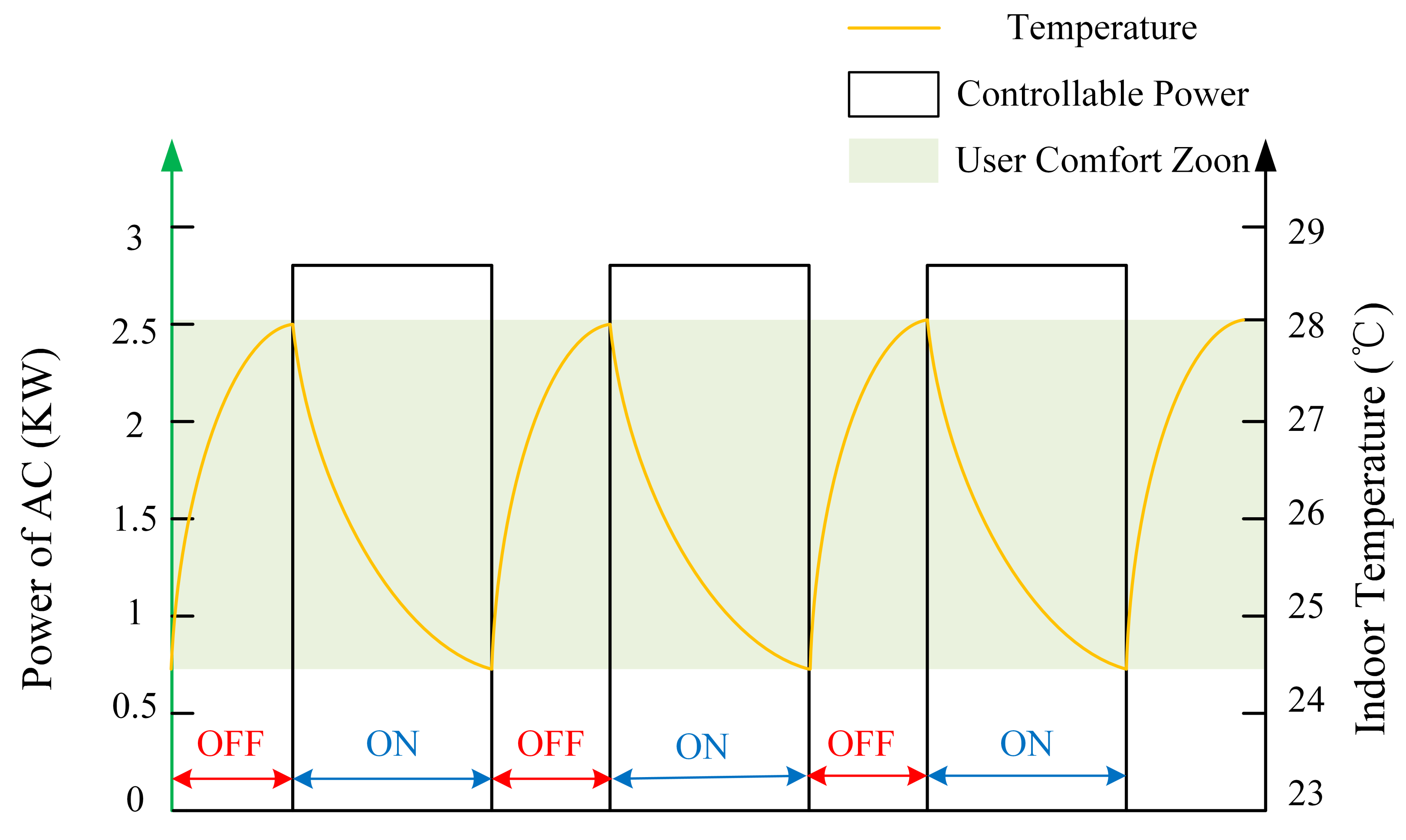
2.1. Cause of Intermittency of DSRs

The intermittency of DSRs’ participation in grid dispatch is a distinctly different characteristic from the responsiveness of generation-side resources. It is typically characterized by the rapid cyclic switching on and off of participating frequency regulation resources within a limited period of time. This is motivated by considerations of user comfort, which means that the response power of DSRs is neither constant at all times nor always sufficient to fulfill grid requirements. In other words, DSRs need to be switched off to help the grid maintain a balance between supply and demand when there is a frequency deviation, and switched on to meet user comfort when their numbers are too low to provide regular service. The classic example is air conditioner (AC).
The AC needs to be maintained in the temperature range between T min , T max to meet the human comfort, from which we can obtain the operating characteristics of the individual ACs in this temperature range and the on/off time parameters as shown in Figure 1. It is worth noting that the intermittent characteristics of DSRs are more often reflected in the large capacity of individual resources, which can be coordinated and optimised to eliminate and mitigate the internal effects of individual resources on each other. However, this does not mean that its intermittent characteristics do not exist. With the large-scale and high-frequency use of DSRs in a short period of time, its intermittency becomes a factor that must be considered.

2.2. Control Strategies for the Intermittent Characteristics of DSRs

Considering that demand-side resources are essentially frequency regulation resources provided by users, when the control center is in frequency regulation, demand-side resources will frequently be in two states of switching on/off, which will lead to certain intermittent characteristics. If a large number of demand-side resources are directly involved in the frequency regulation of the power system without coordination, the simultaneous switching on/off of a large number of resources will cause huge load fluctuations, which will seriously threaten the safety and stability of the power system, and the introduction of large-capacity demand response resources with intermittent characteristics increases the non-linearity of the system. Hence, appropriate control strategies are essential for the steady and safety operation of the grid.
Assuming that the DSRs are involved in primary frequency regulation and that they can detect and respond to grid frequency deviations. With this in mind, the response power of the DSRs can be expressed in Formula (1).
P D S R ( t ) = K ( t ) × Δ f
where P D S R ( t ) denotes the real-time power response of DSRs in frequency regulation, Δ f indicates the deviation of the frequency from the reference value, K ( t ) is the control gain, which is a time-varying function that can be described by Formula (2).
K ( t ) = K , n T t n T + δ 0 , n T + δ < t ( n + 1 )
K R m × n is a constant control gain, T , δ are two parameters to be derived, representing the control period and control width of the DSRs respectively, which affect the stability of the system. when taken large enough the control performance is favorable but sacrificing the user comfort, conversely, when small, the switching frequency is high, which may cause greater damage to the equipment and its repeated switching also causes disturbance to the grid. At the core of the problem lies the design of the intermittent gain K ( t ) . The two remaining parameters, control period T and control width δ > 0 , are related to the type of DSRs and a more detailed derivation is then shown in Section 3.

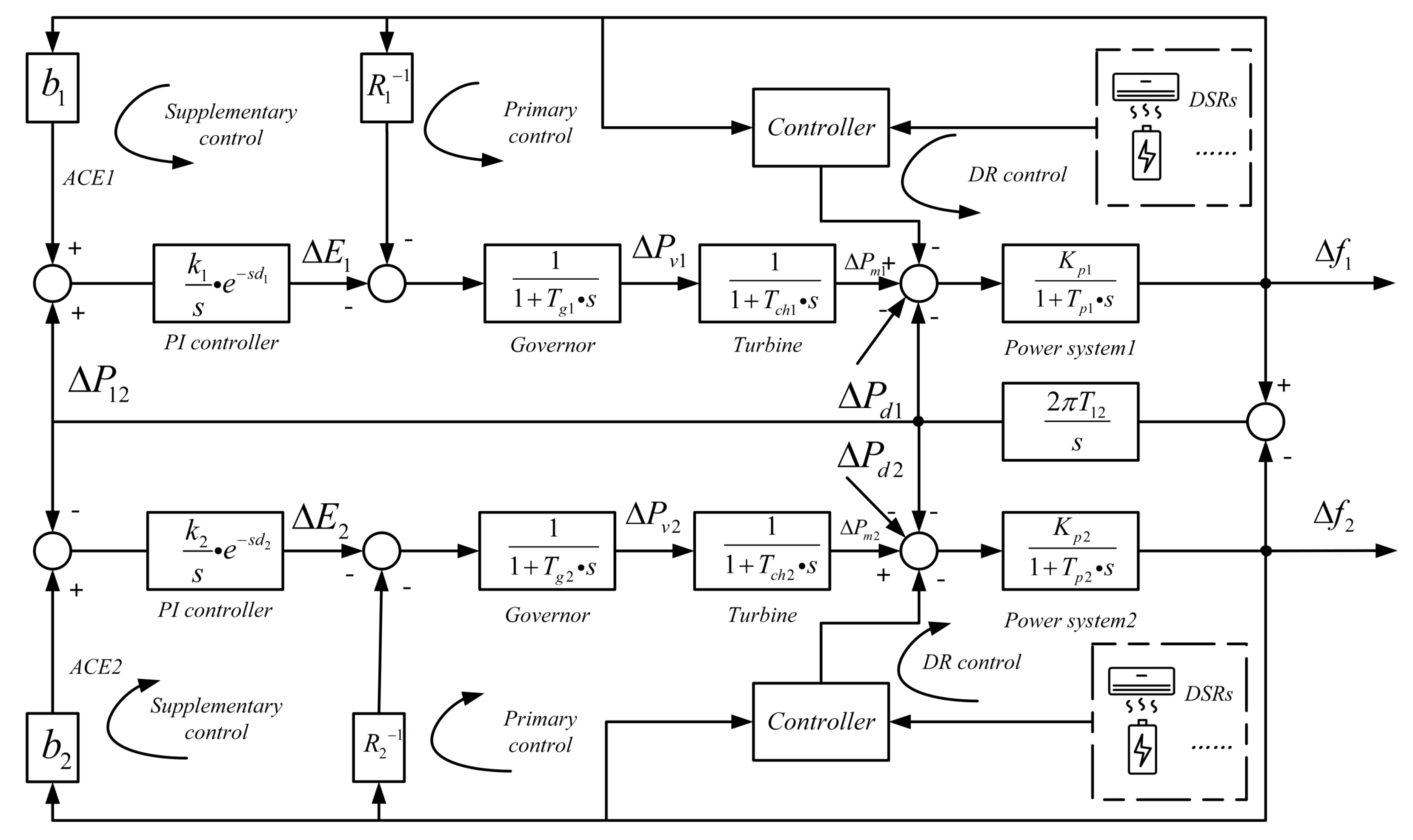
2.3. LFC Model with DSRs

This paper takes a two-region time-lag interconnected power system as the object of study. Considering the intermittent characteristics of the DSRs and the parameter uncertainty due to changes in the balance point during the actual operation of the system, this subsection gives open/closed-loop system models of LFC system.

2.3.1. Open-Loop LFC System Model

Power systems are complex dynamic systems which consist of governors, prime movers, generators, loads, contactors and proportional-integral controllers. The LFC system model for a two-area interconnected system containing DSRs is shown in Figure 2.
In the two-area LFC system model described in Figure 2, Δ E i , Δ P v i , Δ P m i , Δ f i , i = 1 , 2 , , N are power change in secondary frequency control, electromagnetic power deviation, mechanical power deviation, the frequency deviation in area i. Δ P 12 is the tie-line power deviation and Δ P d i is the active change in system load. k i , d i , T g i , T c h i , K p i , T p i , i = 1 , 2 , , N denote control gain in secondary frequency regulation, time lag, time constants for governors, time constants for turbines, system gain, time constants for system in area i. T 12 is the power simultaneous factor of the tie-line between two regions. b i is the regional frequency offset factor and R i is the droop gain in primary frequency control in area i.
As the system usually has multiple delays and is often modelled as a time lag module to simplify the analysis, the system dynamic state–space representation can be described by:
x ˙ ( t ) = A x ( t ) + i = 1 N A i x ( t d i ) + B 1 u 1 m ( t ) + B 2 u 2 n ( t ) + B w w ( t ) z ( t ) = C x ( t ) + D w w ( t )
Considering the errors in system modelling and the uncertainty in power system parameters due to changes in the equilibrium operating point of the power system [20], the above state–space representation can be extended to a model containing the parameter uncertainty terms as follows, namely:
x ˙ ( t ) = ( A + Δ A ) x ( t ) + i = 1 N ( A i + Δ A i ) x ( t d i ) + ( B 1 + Δ B 1 ) u 1 m ( t ) + ( B 2 + Δ B 2 ) u 2 n ( t ) + B w w ( t )
State vectors can be defined as x ( t ) = [ Δ f 1 , Δ P m 1 , Δ P v 1 , Δ E 1 , Δ P 12 , Δ f 2 , Δ P m 2 , Δ P v 2 , Δ E 2 ] A is system matrix, A i , i = 1 , 2 , , N is the matrix of time lag term coefficients, B 1 is the input gain on the generation side, B 2 is the input gain on the DSRs. u 1 m ( t ) is generation-side resources input, while u 2 n ( t ) indicates DSRs input. B w is the gain of the perturbation, which defaults to 1 in this paper. C is the output gain. D w is the direct transmission matrix. N is the number of regions of the LFC system subject to the study, which in this paper is constant 2 Specific parameter data can be found in the Appendix A. To facilitate the design of controller, the parameter uncertainty term is assembled and can be replaced by A ¯ , A i ¯ , B i ¯ for A + Δ A , A i + Δ A i , B i + Δ B i .
To ensure the asymptotic stability of the whole system, we assumed that each region of the system satisfies the following basic assumptions:
  • ( A , B i ) is controllable and r a n k ( B i ) = m i
  • The uncertainty term Δ A , Δ A i , Δ B i is bounded and satisfies max { Δ A , Δ A i , Δ B i } h , where is the norm of the matrix and h is a constant greater than zero. The uncertainty can be described by the following matrix:
[ Δ A , Δ A i , Δ B i ] = H F [ E A , E A i , E B i ]
where the real constant matrix H , E A , E A i , E B i R m × n describing the upper bound on the uncertainty component is known and the matrix F describing the uncertainty is unknown; however, it satisfies the following constraint:
F F T I
Assumption 1 holds, a state feedback controller can be designed whose input u 1 m = [ u 11 , u 12 ] T can be expressed as:
u 1 m ( t ) = L x ( t )
It represents the use of conventional resources (hydro-fired units rotating standby, etc.) in the primary frequency regulation of the system. Next, the controller for the DSRs is designed, and its input u 2 n = [ u 21 , u 22 ] T can be expressed as:
u 2 n ( t ) = K ( t ) x ( t d )
whereby the time lag d of the DSRs is given and the intermittent control gain K ( t ) is the parameter to be found, which can be formulated as Formula (2).

2.3.2. Closed-Loop LFC System Model and Robust H Performance

By substituting u 1 m and u 2 n into Equation (4), the closed-loop state equation of the system can be obtained:
x ˙ ( t ) = A ¯ x ( t ) + i = 1 N A i ¯ x ( t d i ) + B 1 ¯ L x ( t ) + B 2 ¯ K x ( t d ) + B w w ( t ) z ( t ) = C x ( t ) + D w w ( t ) , n T t n T + δ x ˙ ( t ) = A ¯ x ( t ) + i = 1 N A i ¯ x ( t d i ) + B 1 ¯ L x ( t ) + B w w ( t ) z ( t ) = C x ( t ) + D w w ( t ) , n T + δ t ( n + 1 ) T
where L, K and Δ are the controller gains and control width that need to be determined. The robust H performance indicator to be met for the closed-loop Equation (9) is as follows:
J w ( t ) = 0 [ z T ( t ) z ( t ) γ 2 w T ( t ) w ( t ) ] d t < 0
under the initial conditions ϕ ( t ) = 0 , γ > 0 , if there exists an allowable bounded inputs u 1 m , u 2 n such that the system satisfying the above inequality for all permissible parameter uncertainties.

3. Main Result

Based on intermittent control theory [21,22], Section 2.2 and Section 2.3 give a robust controller design scheme for the LFC considering the intermittent characteristics of DSRs. An analysis of the stability and robust H performance of the system is also presented, following the introduction of some common lemmas.

3.1. Preliminaries

Before proceeding to system stability analysis, some common theorems are listed below:
Lemma 1
(Schur Complement [23]). For any given matrix:
A B B C < 0
If A is invertible and satisfies A = A T , C = C T , then the formula above is equivalent to either of the following expressions:
( 1 ) C < 0 , A B C 1 B T < 0 , ( 2 ) A < 0 , D B T A 1 B < 0 .
Lemma 2
([24]). For any real matrix U , V , W R m × n , and matrix M satisfies M = M T , then:
M + U V W + W T V T U T < 0
For all matrices satisfying V V T < I , there exists ε R , ε > 0 , such that the following equation holds:
M + ε 1 U U T + ε W T W < 0
Lemma 3.
An inequality is valid for any vectors x , y R m , positive definite matrix Q R m × n :
2 x T y x T Q x + y T Q 1 y
Lemma 4
(Halanay inequality [25]). Assuming that V : [ μ τ , ) [ 0 , ) is a continuous function and the following inequality is valid:
d V ( t ) d t a V ( t ) + b max V t
is satisfied for t > μ , if a > b > 0 , and then
V ( t ) [ max V μ ] exp { r ( t μ ) } , t μ
where max V t = sup t τ θ t V ( θ ) and r > 0 is the smallest real root of the equation:
r = a + b exp { r τ }
Lemma 5
([26]). Let V : [ μ τ , ) [ 0 , ) be a continuous function such that:
d V ( t ) d t a V ( t ) + b max V t
is satisfied for t > μ ,if a > b > 0 , then:
V ( t ) max V t [ max V μ ] exp { ( a + b ) ( t μ ) } , t μ
where max V t = sup t τ θ t V ( θ )

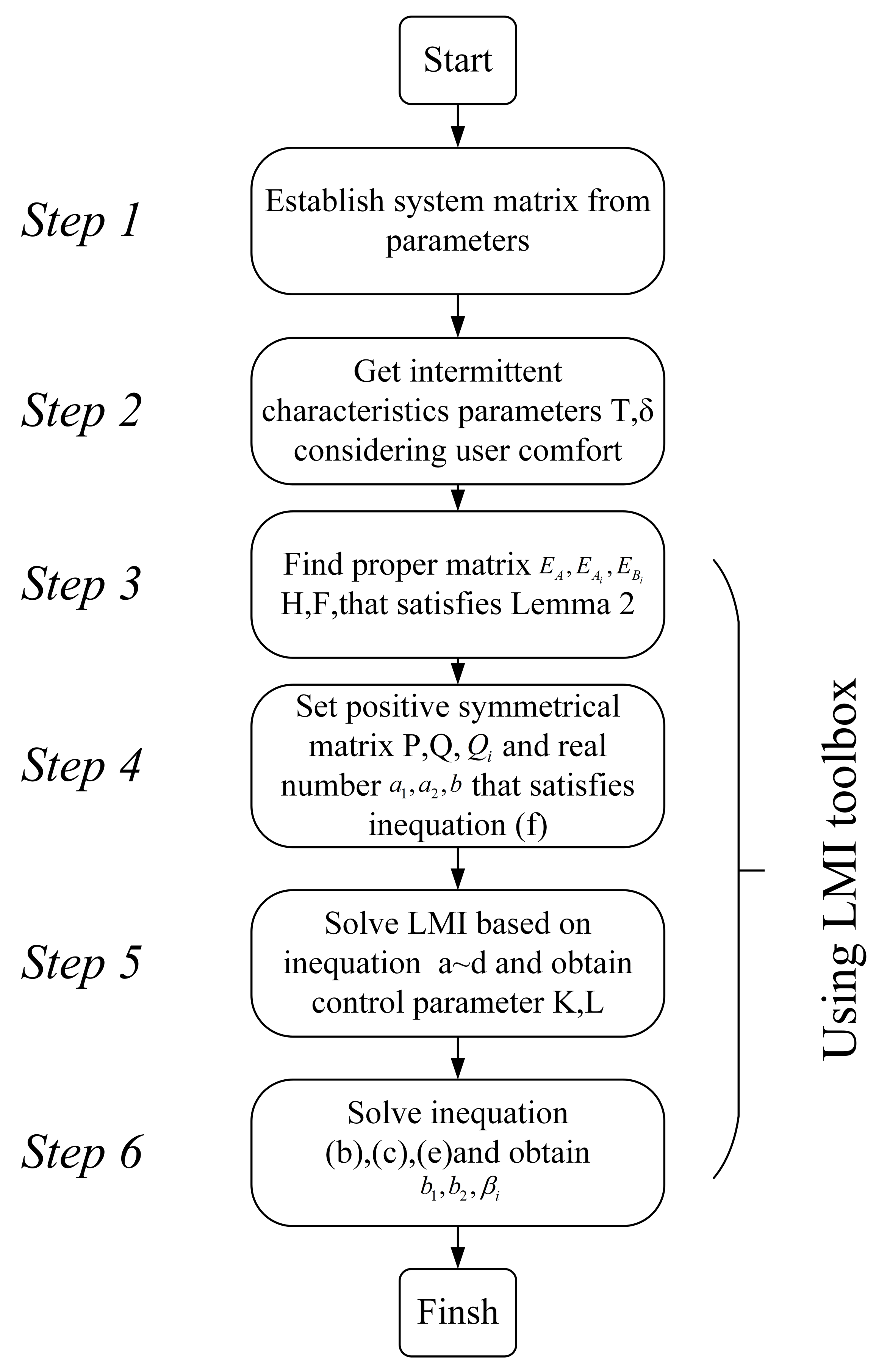
3.2. Controller Design

For any system, stability is a primary prerequisite. This subsection first analyses the stability of the LFC systems accounting for parameter uncertainty and intermittent characteristic DSRs and then gives the design steps for the controller; see Appendix B for a more detailed proof of Theorem 1.
Theorem 1.
An LFC system is exponentially stable if there exist positive definite matrices P = P T , Q = Q T , Q i = Q i T , positive real numbers a 1 , a 2 , β i , b 1 , b 2 , real matrices H, and intermittent control parameters T , δ satisfying the following constraints.
(a)
A X + X T A T + B 1 R + R T B 1 T + a 1 X + M A 1 X A 2 X B 2 Y E A X E B 2 R X A 1 T Z 1 0 0 X A 2 T 0 Z 2 Y T B 2 T Z X T E A T 1 ε 1 I 0 R T E B 2 T 0 0 1 ε 2 I 0
(b)
S i β i X 0 ,
(c)
S β X 0 ,
(d)
A X + X T A T + B 1 R + R T B 1 T a 2 X + M A 1 X A 2 X E A X X A 1 T Z 1 0 0 X A 2 T 0 Z 2 0 X T E A T 0 0 1 ε 1 I 0
(e)
a 1 > b 1 > b 2
(f)
ρ = r ( δ τ ) ( a 2 + b ) ( T δ ) > 0
where r is a positive solution of r = a 1 + b e r τ , τ = max ( d i , d ) , b 1 = i = 1 N β i . Defining the relevant parameters X = P 1 , S i = P 1 Q i 1 P 1 , S = P T Q 1 P 1 , Z i = S i + ε i + 2 X T E A i T E A i X , i = 1 , 2 , the state feedback gains L, and K can be constructed as Y = K X , R = L X . Z = S + ε 5 Y T E B 2 T E B 2 Y , ε 1 , ε 2 , ε 3 , ε 4 , ε 5 are real numbers greater than 0 that satisfy the constraints, M = ( 1 ε 1 + 1 ε 2 + 1 ε 3 + 1 ε 4 + 1 ε 5 ) H H T .
The exponentially stable robust controller parameters can be obtained by solving inequalities (a) to (f), and it is clear that Theorem 1 is a linear matrix inequality constrained feasibility problem that can be solved using the feasp solver in the LMI toolbox.

3.3. Analysis of H Performance

When LFC systems possess H performance, a certain level of stability is still achieved under different perturbations of the system.
Theorem 2.
For a prescribed attenuation level γ > 0 , the LCF system is still asymptotically stable and posses H performance.
Proof of Theorem 1. 
The stability of the closed-loop system Equation (9) under zero initial conditions is analysed below, and it follows easily from the proof of Lemma 1 that, for any non-zero w ( t ) , the following equality holds.
J w ( t ) 0 z T ( t ) z ( t ) γ 2 w T ( t ) w ( t ) + V ˙ ( x t ) d t ξ 1 T ( t ) Π 1 ξ 1 ( t ) d t n T t n T + δ J w ( t ) 0 z T ( t ) z ( t ) γ 2 w T ( t ) w ( t ) + V ˙ ( x t ) d t ξ 2 T ( t ) Π 2 ξ 2 ( t ) d t n T + δ t ( n + 1 ) T
The above equation is equivalent to z 2 2 γ 2 w 2 2 . That is, the system has H performance, where the energy function can be defined as V ( t ) = x T P x , and according to the Lyapunov stability criterion we know that:
V ˙ ( t ) = 2 x T ( t ) P x ˙ ( t ) = 2 x T ( t ) P [ ( A + Δ A ) x ( t ) + i = 1 N ( A i + Δ A i ) x ( t d i ) + ( B 1 + Δ B 1 ) L x ( t ) + ( B 2 + Δ B 2 ) K x ( t d ) ] x T ( t ) [ P A ¯ + A ¯ T P + P B 1 ¯ L + L T B 1 ¯ T P ] x ( t ) + i = 1 N 2 x ( t ) T P A i ¯ x ( t d i ) + 2 x ( t ) T P K x ( t d ) ξ T ( t ) w ξ ( t )
where Π 1 and Π 2 can be expressed as:
1 = A ¯ P 1 + P 1 A ¯ T + B ¯ R + R T B ¯ T + C T C A 1 ¯ A 2 ¯ A N ¯ B ¯ K C T D w + P B w A 1 ¯ T Q 1 1 0 0 0 0 A 2 ¯ T 0 Q 2 1 0 0 0 0 0 A N ¯ T 0 0 Q N 1 0 0 K T B ¯ T 0 0 0 Q 1 0 D T C + B w T P T 0 0 0 0 γ 2 I + D w T D w
and
2 = A ¯ P 1 + P 1 A ¯ T + B ¯ R + R T B ¯ T + C T C A 1 ¯ A 2 ¯ A N ¯ C T D w + P B w A 1 ¯ T Q 1 1 0 0 0 A 2 ¯ T 0 Q 2 1 0 0 0 A N ¯ T 0 0 Q N 1 0 D T C + B w T P T 0 0 0 0 γ 2 I + D w T D w
where ξ 1 T ( t ) = x T ( t ) , x T ( t d 1 ) , , x T ( t d N ) , x T ( t d ) , w ( t ) , ξ 2 T ( t ) = x T ( t ) , x T ( t d 1 ) , , x T ( t d N ) , w ( t ) . □

4. Case Study

A controller demonstrated and analysed from Section 3 will be used in a two-area LFC system [27]. The specific parameters of the 2-zone LFC are shown in Appendix A. Simplifying the analysis, the parameters of Region I and Region II are identical, the time lag is manually set to 0.1 s and the power synchronization factor T 12 is 0.03. Detailed parameters on the simulated system are described in Table 1.

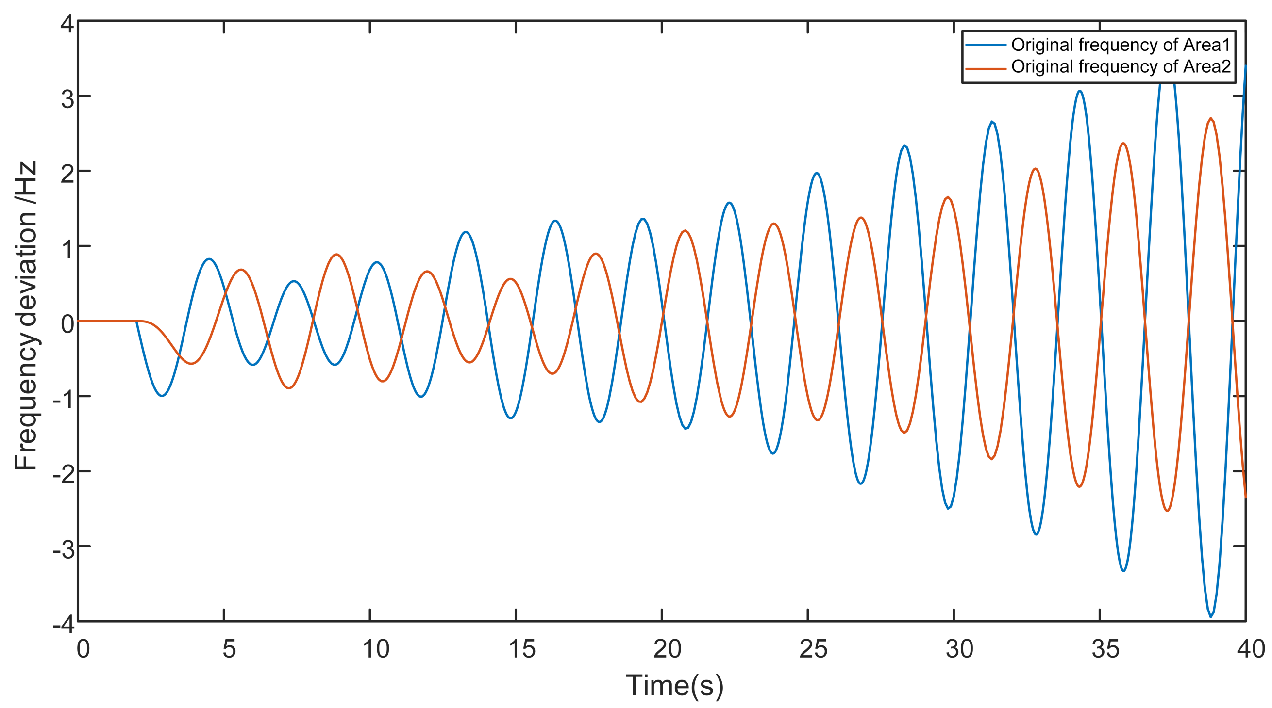
4.1. The Open-Loop LFC System

Assuming that the open-loop LFC Equation (9) has no additional external inputs and is only controlled by proportional integration, i.e., the inputs on the generation and demand sides u 1 m , u 2 n are zero, and a disturbance of 0.5 p.u. is applied in region 1, the frequency deviation of the interconnected LFC system in both regions is shown in Figure 3. Due to the characteristics of the regional interconnection, a disturbance in one of the regions will inevitably affect the frequency stability of the whole network, and thus there is an urgent need for a set of control strategies that can adequately coordinate the generation and demand side resources.

4.2. The Close-Loop LFC System

In order to verify the effectiveness of the proposed control strategy on a closed-loop system, two simulation scenarios are designed to simulate the conditions that may occur in real grid operation. In the first scenario, both generation-side and demand-side resources are invoked, i.e., the DSRs are deployed by the aggregator to assist the grid to achieve power balancing quickly and to ensure the security and stability of the grid operation. In the second scenario, we consider the uncertainty of the system parameters, i.e., the system dynamic equations do not describe the system characteristics and behaviour well due to certain reasons, such as operating point drift and modelling errors. In both scenarios, the control strategy proposed in this paper can be solved by LMI, and the detailed solution steps can be found in Figure 4.

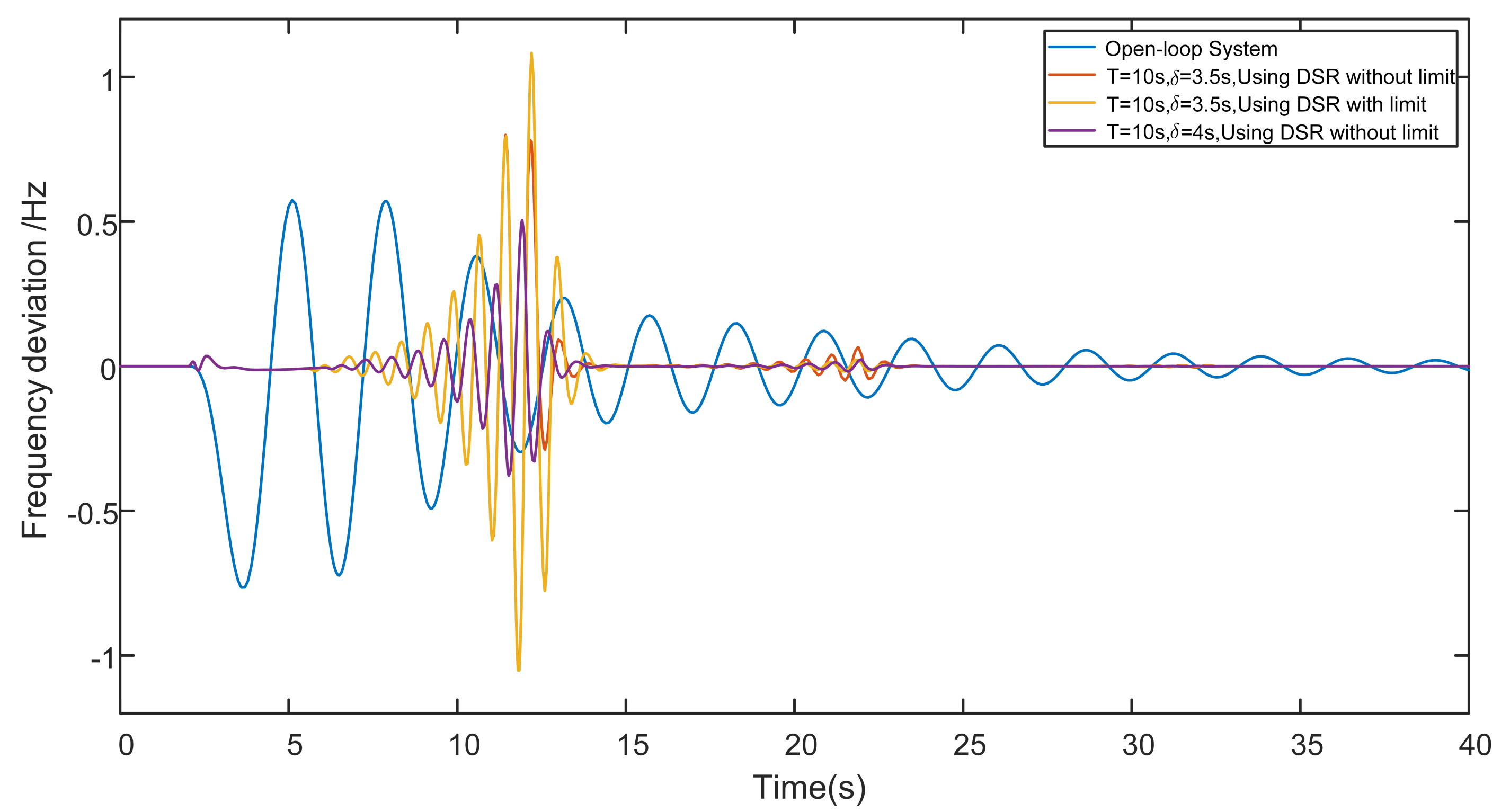
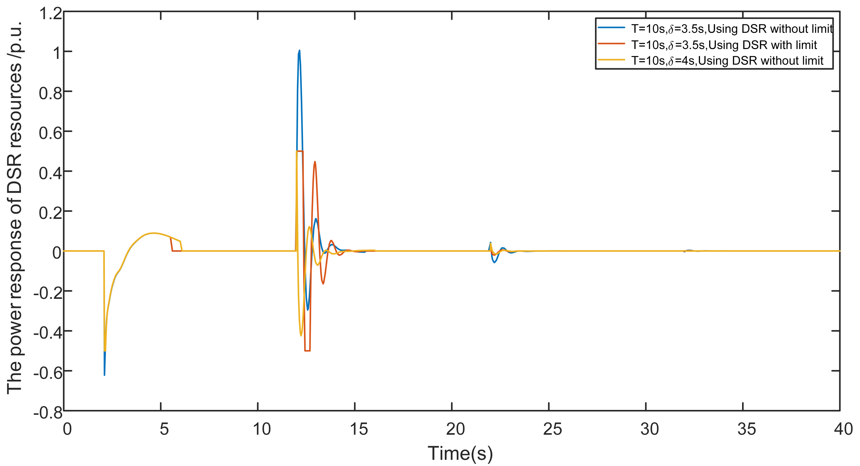
4.2.1. Load-Side and Generation-Side Cooperative Control

In this section, the uncertainty in the system parameters is not considered. We only need to solve equations (a) to (f) in Theorem 1 to get to the corresponding controller parameters, however, before doing so we need to make some reasonable assumptions to reduce the difficulty of solving for the unknown parameters including the positive definite matrix P , Q i , Q , the intermittent control parameters T , δ , and the positive real numbers a 1 , a 2 , β i , b 2 . An initial attempt at a solution was made and we found that it was difficult to converge on a feasible solution due to the high dimensions of the system and the numerous unknown variables. Therefore, two realistic assumptions were made, as described below:
  • As mentioned in Section 2.2, the intermittent control parameters should not only take into account the comfort of the user but also the stability of the system, otherwise the intermittent input itself is a strong source of disturbance for the LFC system, and a review of the relevant literature [28,29] shows that these two parameters are generally a fixed value in a certain region and can be obtained directly.
  • In Formulas (1) and (2) we present the input expression for a DSR resource with intermittent characteristics, which should be related only to the frequency deviation of the system.The DSRs are generally considered to be incapable of detecting any status information other than local frequency deviations in the system, such as the tie line power deviation Δ P 12 and the active change in system load Δ P d i , etc. Therefore, we only need to solve for two parameters.
Figure 4, we first construct the corresponding matrix A , A i , B , C , D based on the structure of the system matrix in the Appendix A. In Step 2 we use Assumption 1, consult the relevant literature and pre-determine the intermittent control parameters T , δ , next we estimate the possible parameter uncertainty and represent it as a combination of a known matrix H , E A , E A i , E B i and an uncertainty matrix F using the constraints in Lemma 2, as discussed in the next section. In step 4, we can specify the positive real numbers a 1 , a 2 , b , the principle being to require a 1 to be as small as possible and a 2 to be as large as possible. A final set of feasible solutions was obtained using the feasp solver.
L = 43 . 05 26 . 04 3 . 39 1110 . 82 784 . 52 22 . 81 10 . 61 1 . 39 1037 . 39 25 . 28 11 . 31 1 . 32 1083 . 02 926 . 72 46 . 16 28 . 41 4 . 22 1405 . 06
K = 2 . 25 0 0 0 0 0 0 0 0 0 0 0 0 0 1 . 33 0 0 0
The simulation scenario remains the same as before and the above parameters are brought into the simulation model. A performance comparison between the open-loop system and the proposed control strategy with different intermittent control parameters T , δ is shown in Figure 5, and the corresponding power response curves of the DSRs are shown in Figure 6.
Figure 5 shows that, as compared to open-loop control, the proposed control strategy is able to reduce the frequency deviation due to load variation, allowing the system frequency to return to the reference value in a limited time. However, in practical engineering, due to the capacity and control width of DSRs, we cannot use the DSRs resources as much as we wish. Therefore, when the input of DSRs does not exceed the disturbance amount, the higher the adjustable capacity of DSR resources, the more powerful the improvement of the grid quality under the same intermittent control parameters. On the other hand, when the control period T is fixed, the control width δ is proportional to the control effect, and conversely, if it is smaller, its own intermittent characteristics are more intense for the grid interference, even when the control width is smaller than a certain threshold, the intermittent control width η = δ / T should be between 40% and 60%, so as to fully exploit the potential of intermittent DSRs without unduly affecting the user comfort.A detailed comparison of control performance can be found in Table 2.
A power response curve for the DSRs is shown in Figure 6. where we can see that the DSRs are constantly switched on/off for a fixed period of time. It is worth noting that without the regulated capacity cap, the demand for DSRs is likely to far exceed the amount of this disturbance itself.

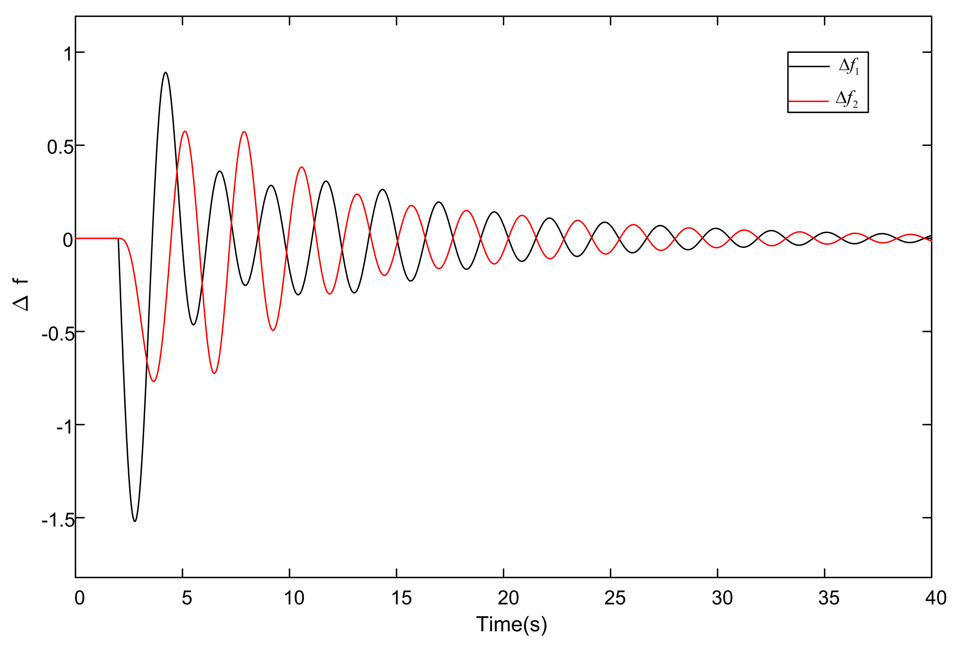
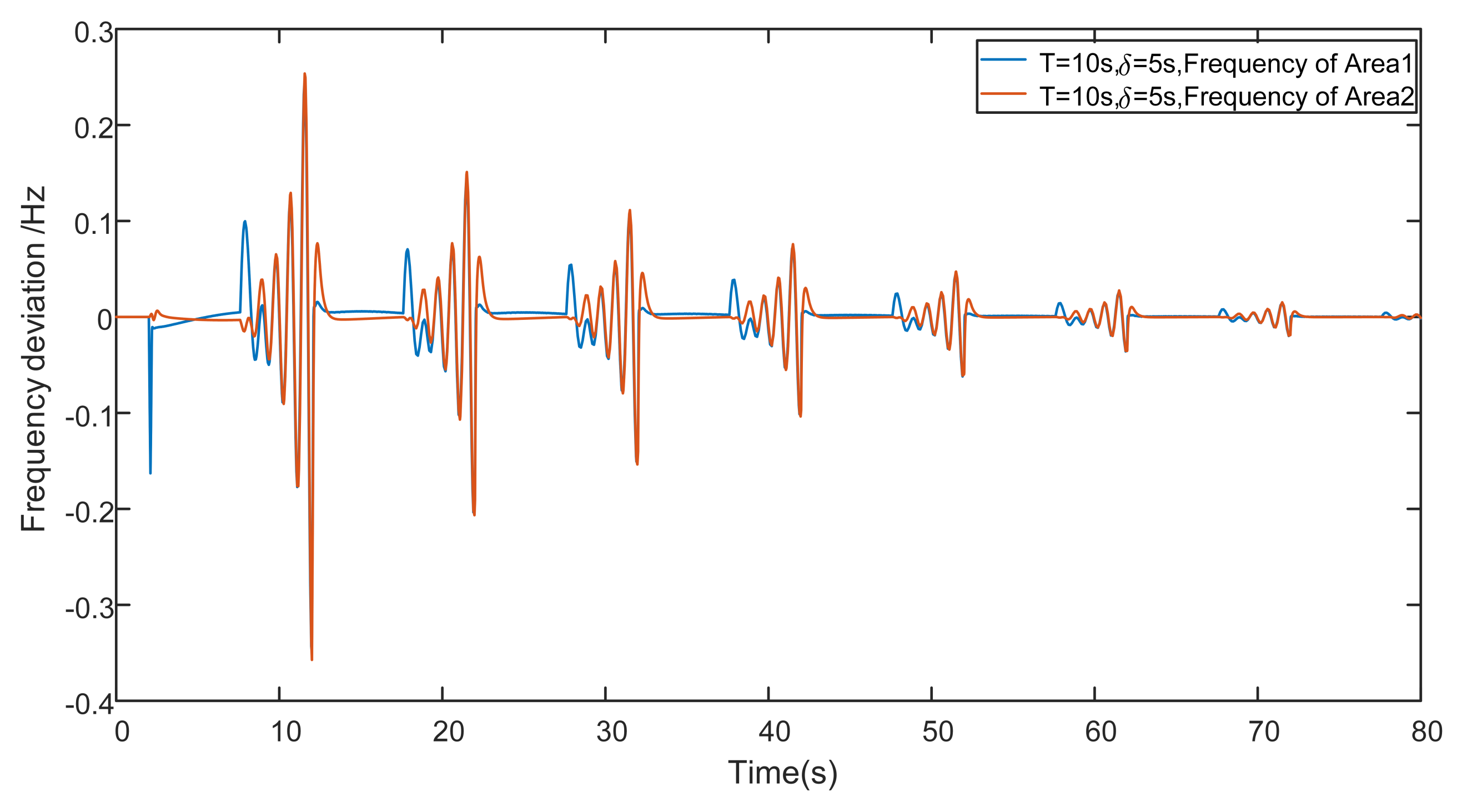
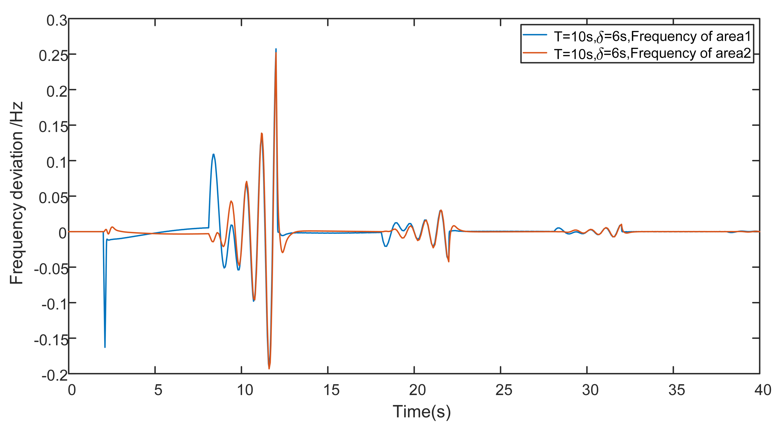
4.2.2. Load-Side and Generation-Side Cooperative Control with Parameter Uncertainty

In this paper, parameter uncertainties due to variations in the operating point of the interconnected LFC system or modelling errors are considered, and the following simulation results show that the control strategy proposed in this paper can improve the robustness of the system. Suppose the system parameters are varied over the range shown below:
T g 1 0.2 0.4 , T g 2 0.25 0.5 , T c h 1 0.22 0.48
T c h 2 0.3 0.46 , K p 1 95 120 , K p 2 95 120
According to Lemma 2, the above parameter uncertainty can be rewritten as a combination of a given parameter H and an uncertain parameter F. We assume that the values of the above parameters are H = 0.1 I , F are matrices satisfying constraint F F T I generated by orthogonal decomposition, and then the system parameters E A , E A i , E B i can be expressed as:
E = F 1 H 1 Δ
where Δ denotes the variation of the system matrix parameters, yielding a set of feasible solutions:
L = 52 . 86 33 . 83 4 . 89 1171 . 59 766 . 23 19 . 94 8 . 62 1 . 02 990 . 97 19 . 59 8 . 11 0 . 63 936 . 96 817 . 82 50 . 91 33 . 39 5 . 59 1333 . 08
K = 18 . 98 0 0 0 0 0 0 0 0 0 0 0 0 0 3 . 69 0 0 0
The simulation scenario is as follows: there exists a certain level of uncertainty in the system parameters that makes it impossible to stabilise the grid frequency in the presence of external disturbances by relying solely on conventional side sources; the specific frequency deviation can be seen in Figure 7.
As shown in Figure 7, a perturbation of 0.5 p.u. is applied in region 1, and the system is no longer stable due to the change in system parameters. The robustness of the control strategy proposed in this paper is tested in the following. The simulation scenario is set up exactly as before, and there are some limitations in the use of DSRs. We tested the system frequency deviation under different intermittent control parameters separately, the curves of frequency variation when the system is subject to perturbations with different parameters are given in Figure 8 and Figure 9, and more detailed data indications can be found in Table 3.
As shown in Figure 8 and Figure 9, when the intermittent control parameter η is small, due to the characteristics of the DSRs themselves, the system frequency decays and oscillates at regular intervals, but eventually stabilises. On the other hand, when the intermittent control parameter is chosen to be larger, the oscillation also occurs, but compared to the former, both the overshoot and the regulation time are substantially improved, and the grid frequency recovers quickly within a short period of time. Noteworthy is that when the intermittency control parameter η is as small as a critical value, not only does it not alleviate the disturbance caused by power loss, but it becomes a strong source of disturbance itself, aggravating the frequency oscillation of the power system.Therefore, in the practical design of the controller, the intermittent control parameters of the DSRs need to be considered, and only when the appropriate parameters are chosen can the best frequency regulation performance be obtained.
We have demonstrated that the system is robust regardless of whether the upper or lower bounds for uncertain parameter variations are taken, based on the design scheme in Section 3.2 Therefore, the load frequency robust controller designed in this paper is insensitive to the uncertainty of the system parameters, has a small overshoot and a short regulation time, which effectively improves the stability of the system.

5. Conclusions

A unique characteristic of DSRs, the intermittent characteristics, is noted, and the reasons for this and its possible adverse impacts on the grid are analysed, followed by a proposed intermittent control strategy for this characteristic, based on which the parameter uncertainties of the system are further considered. Finally, two simulation examples under different scenarios are used to illustrate the effectiveness of the proposed control strategy.
A summary of the full paper is described as follows:
  • The intermittent characteristics of demand-side resources are pervasive and are essentially a compromise of demand response for the comfort of the users, which may affect the steady and safety operation of the power system.
  • Demand-side resources have great potential in grid frequency regulation, pressure on regulation from the generation side would be greatly mitigated if they could be coordinated and complemented with generation-side resources.

Author Contributions

G.M., J.G., J.L., Y.C., K.Y. and K.Z. developed the ideas of this research. G.M., K.Y. and K.Z. performed this research. All authors have read and agreed to the published version of the manuscript.

Funding

This work is supported by State Grid Corporation of China Project “Research on multi-flexible resources collaborative regulation to enhance the consumption capacity of distributed energy(5100-202119576A-0-5-SF)”.

Institutional Review Board Statement

Not applicable.

Informed Consent Statement

Not applicable.

Data Availability Statement

Not applicable.

Conflicts of Interest

The authors declare no conflict of interest.

List of Abbreviations

DSRsDemand-Side Resources
LFCLoad Frequency Conrol
AGCAutomation Generation Control
ACAir Conditioner

Nomenclature

L , K , T , δ Controller parameters to be determined
ε i , a , b Constants greater than zero
Δ E 1 , Δ E 2 Power variation for secondary frequency regulation
Δ P v 1 , Δ P v 2 Electromagnetic power deviation
Δ P m 1 , Δ P m 2 Mechanical power deviation
k i , d i Control gain for secondary frequency regulation, Time lag
T g i , T c h i Governor and turbine time constants
K p i , T p i Power system gain and time constants

Appendix A

This section will give the specific parameters of the matrix mentioned in this paper.
A = 1 T p 1 K p 1 T p 1 0 0 K p 1 T p 1 0 0 0 0 0 1 T c h 1 1 T c h 1 0 0 0 0 0 0 1 T g 1 R 1 0 1 T g 1 0 0 0 0 0 0 k 1 B 1 0 0 0 k 1 0 0 0 0 2 π T 1 0 0 0 0 2 π T 2 0 0 0 0 0 0 0 K p 2 T p 2 1 T p 2 K p 2 T p 2 0 0 0 0 0 0 0 0 1 T c h 2 1 T c h 2 0 0 0 0 0 0 1 T g 2 R 2 0 1 T g 2 0 0 0 0 0 k 2 k 2 B 2 0 0 0
A 1 = 0 2 × 3 0 2 × 1 0 2 × 5 0 1 × 3 1 T g 1 0 1 × 5 0 6 × 3 0 6 × 1 0 6 × 5 A 2 = 0 7 × 8 0 7 × 1 0 1 × 8 1 T g 2 0 7 × 8 0
B 1 = 0 0 1 T g 1 0 0 0 0 0 0 0 0 0 0 0 0 0 1 T g 2 0 T
B 2 = B w = K p 1 T p 1 0 0 0 0 0 0 0 0 0 0 0 0 0 K p 2 T p 2 0 0 0 T
C = 1 0 0 0 0 0 0 0 0 0 0 0 0 0 1 0 0 0 T D w = 0 0

Appendix B

Proof of Theorem 1. 
First, the Lyapunov function, below:
V ( t ) = x T ( t ) P x ( t )
Substitute the closed-loop system model Equation (9) into the above equation and take its derivative with respect to time, for n T t n T + δ , the following results can be derived from applying Lemma 1 and the assumptions:
V ˙ ( t ) = 2 x T ( t ) P x ˙ ( t ) = 2 x T ( t ) P A ¯ x ( t ) + i = 1 N A i ¯ x ( t d i ) + B 1 ¯ L x ( t ) + B 2 ¯ K x ( t d ) x T ( t ) P A ¯ + A ¯ T P + P B 1 ¯ L + L T B 1 ¯ T P x ( t ) + i = 1 N x T ( t ) P A i ¯ Q i A i ¯ T P x ( t ) + i = 1 N x T ( t d i ) Q i 1 x ( t d i ) + x T ( t ) P B ¯ 2 K Q K T B ¯ 2 T P x ( t ) + x T ( t d ) Q 1 x ( t d ) = x T ( t ) [ P A ¯ + A ¯ T P + P B 1 ¯ L + L T B 1 ¯ T P + i = 1 N P A i ¯ Q i A i ¯ T P + P B ¯ 2 K Q K T B ¯ 2 T P + a 1 P ] x ( t ) a 1 x T ( t ) P x ( t ) + i = 1 N x T ( t d i ) ( Q i 1 β 1 P ) x ( t d i ) + i = 1 N x T ( t d i ) β 1 P x ( t d i ) + x T ( t d ) ( Q 1 b 2 P ) x ( t d ) + x T ( t d ) b 2 P x ( t d ) < a 1 V ( t ) + i = 1 N β i V ( t d i ) + b 2 V ( t d )
The next step is to prove that the above Formula (A2) is negative definite, Let:
Ω P A ¯ + A ¯ T P + P B 1 ¯ L + L T B 1 ¯ T P + i = 1 N P A i ¯ Q i A i ¯ T P + P B ¯ 2 K Q K T B ¯ 2 T P + a 1 P
Pre and post multiply P 1 to Ω and substitute with the following variables: R = L P 1 , X = P 1 , S i = P 1 Q i 1 P 1 , S = P T Q 1 P 1 . Then we can convert Ω 0 to:
( A + Δ A ) X + X T ( A + Δ A ) T + ( B 1 + Δ B 1 ) L X + X T L T ( B 1 + Δ B 1 ) T + i = 1 N ( A i + Δ A i ) X S i 1 X T ( A i + Δ A i ) T + ( B 2 + Δ B 2 ) K X S 1 X T K T ( B 2 + Δ B 2 ) T + a 1 X 0
Applying the Schur complement, we might discover that Ω 0 is identical to condition (a). An advantage of this is that matrix inequalities of high dimension can be simplified to a series of LMI inequalities that can be easily solved by computer iteration. Using conditions (a)–(c) and (A2), one concludes the following:
V ˙ ( t ) < a 1 V ( t ) + i = 1 N β i V ( t d i ) + b 2 V ( t d ) n T t n T + δ V ˙ ( t ) < a 2 V ( t ) + i = 1 N β i V ( t d i ) n T + δ t ( n + 1 ) T
Alternatively, the closed-loop system Equation (9) can be considered to possess robust H performance by ensuring that it is exponentially asymptotically stable with w ( t ) = 0 .
By condition (a), (c), (d), the following conclusions can be drawn:
V ˙ ( t ) < a 2 V ( t ) + b 1 max V t
where, τ = max ( d i , d ) , b = b 1 + b 2 , b 1 = i = 1 N β i
Moving on, merely ensure that the error e ( t ) 0 , From Lemma 2 and (A2), One could easily conclude that:
V ( t ) τ max t τ θ t V ( θ )
the following conclusions can be drawn:
V ( t ) V ( 0 ) τ e r t , 0 t δ
where r is the unique positive solution of r = a 1 + b e r τ , by Lemma 4:
V ( t ) V ( δ ) τ e ( a 2 + b ) ( t δ ) = max δ τ t δ V ( t ) e ( a 2 + b ) ( t δ ) V ( 0 ) τ e r ( δ t ) e ( a 2 + b ) ( t δ )
for δ t T , assuming that T τ > δ then:
V ( T ) τ = max T τ t T V ( t ) max T τ t T V ( 0 ) τ e r ( δ t ) e ( a 2 + b ) ( t δ ) = V ( 0 ) τ e r ( δ t ) e ( a 2 + b ) ( T δ ) = V ( 0 ) τ e ρ
Using mathematical induction, we can prove, for any positive integer n, here is the formula that certainly holds:
V ( n T ) τ V ( 0 ) τ e n ρ
There is one main premise, assume Formula (A8) holds when k < n . Now, we prove Formula (A8) is valid when k = n + 1 .
First, when t [ n T , n T + δ ] , we have:
V ( t ) V ( n T + δ ) τ e ( a 2 + b ) ( t n T δ ) = [ max n T + δ τ t n T + δ V ( t ) ] e ( a 2 + b ) ( t n T δ ) [ max n T + δ τ t n T + δ V ( 0 ) τ e n ρ e r ( t n T ) ] e ( a 2 + b ) ( t n T δ ) V ( 0 ) τ e n ρ e r ( t n T ) e ( a 2 + b ) ( t n T δ )
and
V ( ( n + 1 ) T ) τ = max ( n + 1 ) T τ t ( n + 1 ) T V ( t ) max ( n + 1 ) T τ t ( n + 1 ) T V ( 0 ) τ e n ρ e r ( t n T ) e ( a 2 + b ) ( t n T δ ) = V ( 0 ) τ e n ρ e r ( δ t ) e ( a 2 + b ) ( T δ ) = V ( 0 ) τ e ( n + 1 ) ρ
Thus, Equation (A8) holds for all positive integers k. For any t > 0 , there is n 0 > 0 , such that n 0 T t ( n 0 + 1 ) T .
V ( t ) V ( n 0 T ) τ e ( a 2 + b ) ( t n 0 T ) V ( 0 ) τ e n 0 ρ e ( a 2 + b ) T V ( 0 ) τ e ( a 2 + b ) T e ρ e ρ T t
Let M = V ( 0 ) τ e ( a 2 + b ) T e ρ , we have:
λ m ( p ) x ( t ) 2 V ( t ) M e ρ T t , t 0
Clearly,
x ( t ) M λ m e ρ 2 T t .

References

  1. Shayeghi, H.A.S.H.; Shayanfar, H.A.; Jalili, A. Load frequency control strategies: A state-of-the-art survey for the researcher. Energy Convers. Manag. 2009, 50, 344–353. [Google Scholar] [CrossRef]
  2. Meng, L.; Zafar, J.; Khadem, S.K.; Collinson, A.; Murchie, K.C.; Coffele, F.; Burt, G.M. Fast Frequency Response From Energy Storage Systems Review of Grid Standards, Projects and Technical Issues. IEEE Trans. Smart Grid 2020, 11, 1566–1581. [Google Scholar] [CrossRef] [Green Version]
  3. Yao, J.G.; Zhang, K.F.; Ding, Z.T.; Li, Y.P.; Yang, S.C.; Xia, M. Concept Extension and Research Focus of Dynamic Demand Response. Autom. Electr. Power Syst. 2019, 43, 9. (In Chinese) [Google Scholar]
  4. Short, J.A.; Infield, D.G.; Freris, L.L. Stabilization of Grid Frequency Through Dynamic Demand Control. IEEE Trans. Power Syst. 2007, 22, 1284–1293. [Google Scholar] [CrossRef] [Green Version]
  5. Vardakas, J.S.; Zorba, N.; Verikoukis, C.V. A Survey on Demand Response Programs in Smart Grids: Pricing Methods and Optimization Algorithms. IEEE Commun. Surv. Tutor. 2015, 17, 152–178. [Google Scholar] [CrossRef]
  6. Gao, C.; Liang, T.; Li, Y. A Survey on Theory and Practice of Automated Demand Response. Power Syst. Technol. 2014, 38, 8. (In Chinese) [Google Scholar]
  7. Shen, Y.; Li, Y.; Gao, C.; Zhou, L. Application of Demand Response in Ancillary Service Market. Autom. Electr. Power Syst. 2017, 41, 11. (In Chinese) [Google Scholar]
  8. Han, B.; Yao, J.; Yu, Y. Discussion on Active Load Response at Receiving End Power Grid for Mitigating UHVDC Blocking Fault. Autom. Electr. Power Syst. 2016, 40, 6. (In Chinese) [Google Scholar]
  9. Pourmousavi, S.A.; Nehrir, M.H. Introducing Dynamic Demand Response in the LFC Model. IEEE Trans. Power Syst. 2014, 29, 1562–1572. [Google Scholar] [CrossRef]
  10. Yi, T.; Feng, L.; Qian, C.; Li, M.; Qi, W.; Ming, N.; Gang, C. Frequency prediction method considering demand response aggregate characteristics and control effects. Appl. Energy 2018, 229, 936–944. [Google Scholar]
  11. Molina-Garcia, A.; Bouffard, F.; Kirschen, D.S. Decentralized Demand-Side Contribution to Primary Frequency Control. IEEE Trans. Power Syst. 2011, 26, 411–419. [Google Scholar] [CrossRef]
  12. Liu, H.; Huang, K.; Wang, N.; Qi, J.; Wu, Q.; Ma, S.; Li, C. Optimal dispatch for participation of electric vehicles in frequency regulation based on area control error and area regulation requirement. Appl. Energy 2019, 240, 46–55. [Google Scholar] [CrossRef]
  13. Bai, L.; Li, F.; Cui, H.; Jiang, T.; Sun, H.; Zhu, J. Interval optimization based operating strategy for gas-electricity integrated energy systems considering demand response and wind uncertainty. Appl. Energy 2016, 167, 270–279. [Google Scholar] [CrossRef] [Green Version]
  14. Zhao, C.; Wang, J.; Watson, J.P.; Guan, Y. Multi-stage robust unit commitment considering wind and demand response uncertainties. In Proceedings of the IEEE PES General Meeting, Conference & Exposition, Virtual Event, 26–29 July 2021. [Google Scholar]
  15. Ziping, W.U.; Gao, W.; Gao, T.; Yan, W.; Wang, X. State-of-the-art review on frequency response of wind power plants in power systems. J. Mod. Power Syst. Clean Energy 2018, 6, 1–16. [Google Scholar]
  16. Han, Z.; He, R.; Xu, Y. Study on Resonance Mechanism of Power System Low Frequency Oscillation Induced by Turbo-pressure Pulsation. Proc. CSEE 2008, 28, 5. (In Chinese) [Google Scholar]
  17. Milano, F.; Zarate-Minano, R. A Systematic Method to Model Power Systems as Stochastic Differential Algebraic Equations. IEEE Trans. Power Syst. 2013, 28, 4537–4544. [Google Scholar] [CrossRef]
  18. Sun, Y.; Zhao, X.; Ning, L.; Wei, Z.; Sun, G. Robust stochastic stability of power system with time-varying delay under Gaussian random perturbations. Neurocomputing 2015, 162, 1–8. [Google Scholar] [CrossRef]
  19. Mi, Y.; Fu, Y.; Li, D.; Wang, C.; Loh, P.C.; Wang, P. The sliding mode load frequency control for hybrid power system based on disturbance observer. Int. J. Electr. Power Energy Syst. 2016, 74, 446–452. [Google Scholar] [CrossRef]
  20. Preece, R.; Woolley, N.C.; Milanovic, J.V. The Probablistic Collocation Method for Power System Damping and Voltage Collapse Studies in the Presence of Uncertainties. IEEE Trans. Power Syst. 2013, 28, 2253–2262. [Google Scholar] [CrossRef]
  21. Xia, W.; Cao, J. Pinning synchronization of delayed dynamical networks via periodically intermittent control. Chaos 2009, 19, 821–891. [Google Scholar] [CrossRef]
  22. Żochowski, M. Intermittent dynamical control. Phys. D Nonlinear Phenom. 2000, 145, 181–190. [Google Scholar] [CrossRef]
  23. Boyd, S.; El Ghaoui, L.; Feron, E.; Balakrishnan, V. Linear Matrix Inequalities in System and Control Theory; Studies in Applied Mathematics; SIAM: Philadelphia, PA, USA, 1994; Volume 15. [Google Scholar]
  24. Xie, L.; Fu, M.; Souza, C.D. H control and quadratic stabilization of systems with parameter uncertainty via output feedback. Autom. Control IEEE Trans. 1992, 37, 1253–1256. [Google Scholar] [CrossRef]
  25. Halanay, A. Differential equations: stability, oscillations, time lags. Siam Rev. 1975, 10, 93–94. [Google Scholar]
  26. Li, C.; Liao, X.; Huang, T. Exponential stabilization of chaotic systems with delay by periodically intermittent control. Chaos Interdiscip. J. Nonlinear Sci. 2007, 17, 043103. [Google Scholar] [CrossRef]
  27. Liu, Z.W.; Yu, X.; Guan, Z.H.; Hu, B.; Li, C. Pulse-Modulated Intermittent Control in Consensus of Multiagent Systems. IEEE Trans. Syst. Man Cybern. Syst. 2016, 47, 1–11. [Google Scholar] [CrossRef]
  28. Hu, X. Research on Modeling and Control Strategy for Air Conditioning Loads to Participate in Demand Response in Power System. Ph.D. Thesis, Southeast University, Nanjing, China, 2017. (In Chinese). [Google Scholar]
  29. Lei, Z.; Yang, L.; Ciwei, G. Improvement of Temperature Adjusting Method for Aggregated Air-conditioning Loads and Its Control Strategy. Proc. CSEE 2014, 34, 5579–5589. (In Chinese) [Google Scholar]
Figure 1. Classic intermittent DSRs: Air Conditioner.
Energies 15 04370 g001
Figure 2. Two-area LFC system with DSRs.
Energies 15 04370 g002
Figure 3. Frequency deviation in LFC open-loop system.
Energies 15 04370 g003
Figure 4. Detailed solution process of control parameter K and L.
Energies 15 04370 g004
Figure 5. Frequency deviation of area 2.
Energies 15 04370 g005
Figure 6. The response power of DSRs.
Energies 15 04370 g006
Figure 7. Frequency deviation of the LFC system considering parameter uncertainty with No control input.
Energies 15 04370 g007
Figure 8. Frequency deviation of the LFC system when δ = 5 s.
Energies 15 04370 g008
Figure 9. Frequency deviation of the LFC system when δ = 6 s.
Energies 15 04370 g009
Table 1. Parameters of a two-area LFC system.
Area K pi T pi T chi T gi b i R i k i d i
1120200.310.250.4252.40.670.1
1120200.30.30.4252.40.60.1
Table 2. Comparison of results for control performance.
MethodMaximum Frequency DeviationTransient Time
Open-Loop System0.78 Hz36.5 s
This Paper ( δ = 3.5 s)0.72 Hz23.5 s
This Paper ( δ = 4 s)0.52 Hz21.5 s
Table 3. Comparison of the control performance results under parameter uncertainty.
MethodMaximum Frequency DeviationTransient Time
Open-Loop SystemUnstable system()Unstable system()
This Paper ( δ = 5 s)0.35 Hz72 s
This Paper ( δ = 6 s)0.19 Hz33 s
Publisher’s Note: MDPI stays neutral with regard to jurisdictional claims in published maps and institutional affiliations.

