Online Estimation of Open Circuit Voltage Based on Extended Kalman Filter with Self-Evaluation Criterion

Abstract

Open circuit voltage (OCV) is crucial for battery degradation analysis. However, high-precision OCV is usually obtained offline. To this end, this paper proposes a novel self-evaluation criterion based on the capacity difference of State of Charge (SoC) unit interval. The criterion is integrated into extended Kalman filter (EKF) for joint estimations of OCV and SoC. The proposed method is evaluated in a typical application scenario, energy storage system (ESS), using a ${\mathrm{LiFePO}}_4$ (LFP) battery. Extensive experimental results show that a more accurate OCV and incremental capacity and differential voltage (IC-DV) can be achieved online with the proposed method. Our method also greatly improves the accuracy of SoC estimation at each SoC point where the maximum estimation error of SoC is less than 0.3%.

1. Introduction

Recently, lithium-ion batteries have been widely used in electric vehicles (EV) and energy storage systems (ESS). With the increasing use of lithium-ion batteries, fire incidents in EV and ESS also occur more frequently, which makes the safety of lithium-ion batteries an increasing concern for society. Moreover, degradation of the lithium-ion batteries will inevitably occur with the aging of the batteries. If the process, degree and path of battery degradation cannot be detected online in time, it will seriously threaten the safety and reliability of the battery system.

Many studies have focused on the degradation mechanism (DM) analysis of lithium-ion batteries [1,2,3,4,5,6,7,8]. Among these analytical approaches, the analyses of the incremental capacity and differential voltage (IC-DV) curves, i.e., $dQ/dV$ (IC) and $dV/dQ$ (DV) curves, are the most widely used approaches in DM analysis [2,8,9,10,11,12]. The IC-DV curves can be obtained from the derivatives of the open circuit voltage (OCV) curve. The IC-DV curves magnify the details of the OCV curve. Through analysis of the shift and the magnitude change of the peaks of the IC-DV curves, the process, degree and path of battery degradation can be obtained.

OCV and IC-DC curves are mostly obtained by offline approaches [4,13,14]. The controllable current in an offline environment makes it easier to obtain the OCV and IC-DV curves. However, the current is uncontrollable in real applications where accurate OCV and IC-DV curves are more difficult to obtain. Although offline approaches help us to understand the mechanism and process of the battery degradation, online estimation of the OCV and IC-DV curves with high precision is more helpful to achieve the actual status of the battery degradation, which is of great significance in ensuring the safety of the battery, predicting the remaining useful life (RUL) of the battery and evaluating the residual value of the battery for recycling and re-utilization. There are also some approaches which estimate the OCV curve online [15,16,17,18,19,20,21]. However, due to the drastic change of the current in real applications, high-precision online OCV estimation is difficult to achieve.

The main contribution of this paper is that we propose a novel algorithm framework to achieve high-precision online OCV estimation which can meet the requirement of online battery degradation analysis. Meanwhile, our method also greatly improves the estimation accuracy of state of charge (SoC).

The paper is organized as follows. Section 2 introduces the related work of OCV curve modeling, offline measurement and online estimation. Section 3 briefly introduces the extended Kalman filter (EKF) algorithm for SoC estimation. Then, a novel self-evaluation criterion is introduced. We propose a novel algorithm framework to combine EKF with the self-evaluation criterion for the joint estimations of the OCV and SoC. Experimental results of the proposed algorithm framework on different scenarios are presented in Section 4. Section 5 summarizes the conclusions and future work.

2. Related Work

The OCV curve is commonly defined as the voltage difference measured between the positive electrode (PE) and the negative electrode (NE) at each SoC point when there is no external current flow and the electrode potentials are at equilibrium status. The OCV curve is an important parameter in various battery models. For battery-model-based SoC estimation, such as EKF, the accuracy of the OCV curve can determine the accuracy of the SoC estimation. Moreover, the OCV curve also reflects the thermodynamic information of the electrode and the amount of lithium intercalated in any given phase. The thermodynamic information of the electrode includes the number and the types of the phase transitions undergone by electrode materials during charging and discharging. The characteristics of the thermodynamic information has attracted great interests for modeling lithium-ion battery [6,22,23,24,25].

The OCV curve is generally obtained offline. Galvanostatic Intermittent Titration Technique (GITT) and pseudo-OCV test are two approaches widely used to obtain the OCV curve. Through these two approaches, we can obtain the OCV value of each corresponding SoC point. In GITT method, the step of charging or discharging and the duration of relaxation to obtain the OCV curve are two important parameters. To obtain a more accurate OCV curve, a finer step and a longer relaxation time are necessary. Barai et al. [13] suggested setting the duration of relaxation to 4 h for battery to reach a state close to equilibrium. A relaxation time of 40 h is even suggested when measuring the OCV of ${\mathrm{LiFePO}}_4$ (LFP) [14], which only brings marginal improvement of the accuracy of the SoC estimation. Therefore, there needs a trade-off between the accuracy of the SoC estimation and the relaxation time used to obtain the OCV curve. A pseudo-OCV test is another way to obtain the OCV curve. By applying a small charging or discharging current to the battery, typically $C/25$ or lower, the OCV curve named pseudo-OCV curve can be obtained. By applying a small current, the kinetic contributions and ohmic heat generation are reduced. Moreover, the electrode polarization is lowered. A more detailed description and comparison of these two approaches can be found in Barai et al. [4].

Many approaches are proposed to model the OCV curve. Starting with the simplest linear approximation model, a variety of models are designed to fit the real OCV curve. Polynomial models are used to fit the OCV curve in [26,27]. The greater the order of the polynomial, the more precise the model. However, high-order polynomial models are difficult to implement in Battery Management System (BMS). More complex models which combine polynomial, exponential and logarithmic functions are proposed [28,29,30]. Recently, the research of lithium-ion battery degradation has put forward high demands for the accuracy of the OCV curve, which also complicates the modeling of the OCV [31]. Table 1 summarizes several typical OCV models.

Table 1. Overview of OCV models.

OCV Curve Fitting Formula	Ref.
$OCV\left(x\right)=K_0-K_1/x-K_{2}x+K_{3}ln\left(x\right)+K_{4}ln(1-x)$	[28]
$OCV\left(x\right)=K_0+K_1(1-e^{-{\alpha }_{1}x})+K_2(1-e^{-\frac{{\alpha }_2}{(1-x)}})+K_{3}x$	[30]
$OCV\left(x\right)=K_0+K_1{e}^{-{\alpha }_{1}x}+K_{2}x+K_3{x}^2+K_4{x}^3$	[29]
$OCV\left(x\right)=K_0+K_{1}x+K_2{x}^2+K_3{x}^3+K_4{x}^4+K_5{x}^5+K_6{x}^6$	[26]
$OCV\left(x\right)=K_0+K_1\frac{1}{1+e^{{\alpha }_1(x-{\beta }_1)}}+K_2\frac{1}{1+e^{{\alpha }_2(x-{\beta }_2)}}+K_3\frac{1}{1+e^{{\alpha }_3(x-1)}}+K_4\frac{1}{1+e^{{\alpha }_{4}x}}+K_{5}x$	[31]

There are also some works online which estimate the OCV curve. He et al. [15] proposed an online model-based SoC estimation method based on online identification of OCV. Tong et al. [16] designed a state/parameter dual estimator and seamlessly integrated EKF, recursive least Square (RLS) and a parameter-varying approach (PVA). RLS was used in [16] to track the battery OCV value and internal resistance value. With the online optimization of the OCV curve, the accuracy of SoC estimation was improved by 0.5–3% in studied cases. In [17], an online estimation method of model parameters was proposed by using an adaptive control approach. The adaptive control approach is widely employed in non-linear control systems with uncertain parameters. Two different adaptive filtering methods (recursive least square, RLS, and least mean square, LMS) are designed to achieve online OCV estimation in [18]. Ref. [19] proposed a method for rapid estimation of battery aging states and reconstruction of the open circuit voltage-charge amount (OCV-Q) curves. Convolutional neural network (CNN) is leveraged to estimate the electrode aging parameters (EAPs). With the estimated EAPs, OCV-Q curves can be reconstructed at different aging levels with a root mean square error (RMSE) of less than 15 mV. In [20], an OCV reconstruction method is presented to update the OCV curve for SoC estimation. To obtain more stable parameter identification to reconstruct the OCV curve, a parameter identification method with parameter backtracking strategy is proposed to reduce the jitters of the parameters. Using the OCV reconstruction method, the SoC estimation errors are within $3\%$. Xiong et al. proposed a method to extract the OCV and OCV-SoC relationship from any current-voltage measurements of full charge/discharge process data [21]. The previous charge and discharge data are used to improve the accuracy of the estimated OCV-SoC relationship. The SoC error is less than $1\%$ in [21]. Earlier work of online OCV estimation aims to improve the accuracy of SoC estimation through online OCV estimation. More recent works are focused on improving the accuracy and smoothness of the estimated OCV itself. However, it is still challenging to achieve high-precision online OCV estimation.

In this paper, a novel self-evaluation criterion based on the capacity difference of the SoC unit interval is proposed. This self-evaluation criterion not only focuses on the mean absolute error (MAE) or root mean square error (RMSE) of SoC, but also describes the SoC error of each point in detail. By combining this self-evaluation criterion with EKF-based SoC estimation, we build a novel algorithm framework for high-precision joint estimations of SoC and OCV curve. By comparing the OCV curve and the IC-DV curves estimated by our proposed method with the curves obtained by pseudo-OCV testing, it can be observed that the accuracy of our OCV curve estimation can meet the requirement for online battery degradation.

3. Proposed Method

In this section, we first briefly introduce the EKF algorithm for SoC estimation. Then, we introduce our self-evaluation criterion, where the difference between our self-evaluation criterion and traditional evaluation criterion are explained. Finally, the self-evaluation criterion is integrated into the framework of EKF for OCV and SoC estimations.

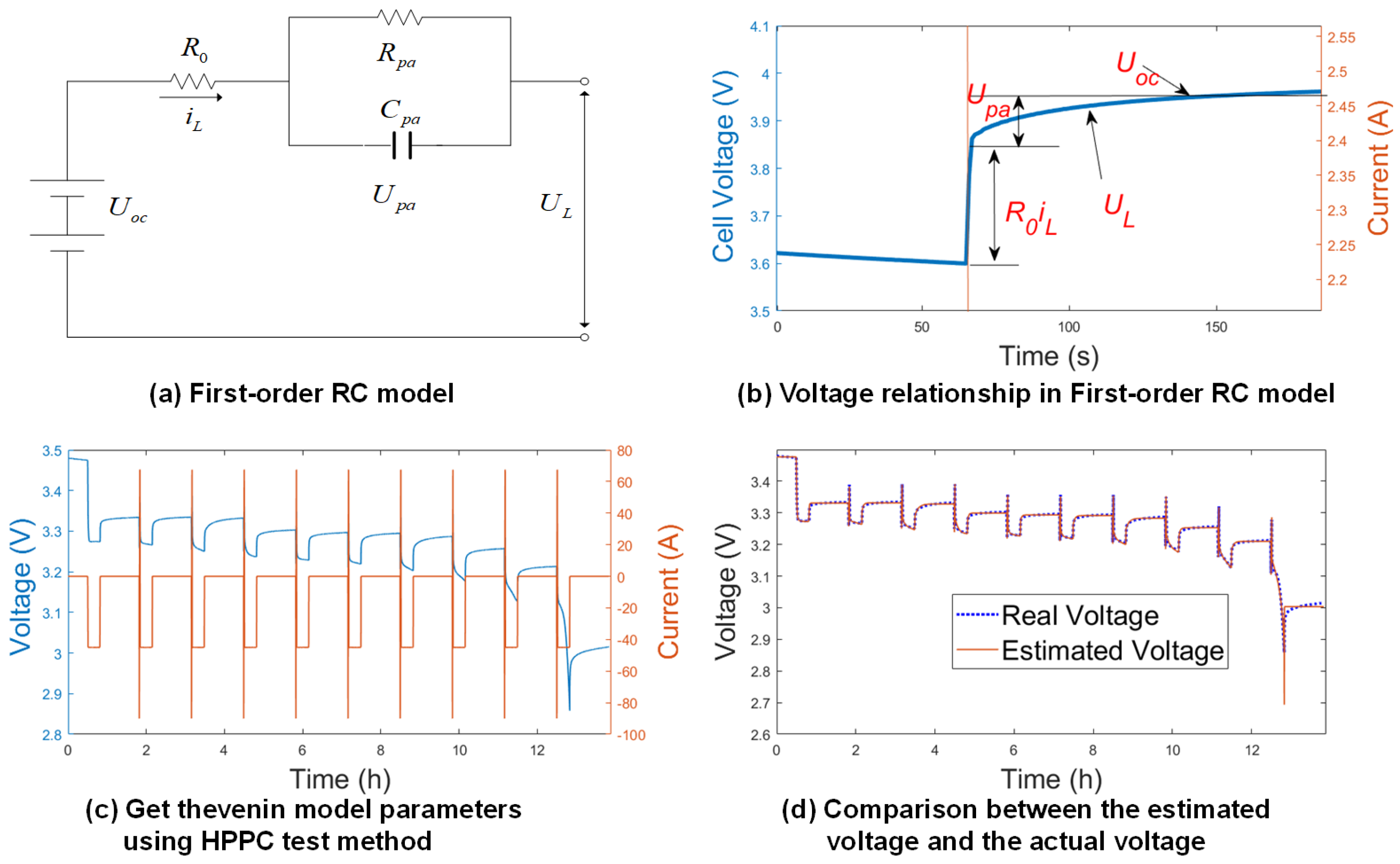
3.1. Extended Kalman Filter in SoC Estimation

Among many SoC estimation algorithms, EKF-based approaches [28] and its derivatives, such as unscented Kalman filter (UKF) [32], sigma-point Kalman filter (SPKF) [33], are widely used approaches in both academia and industry. EKF-based approaches address the problem of error accumulation in the coulomb counting method. Moreover, EKF-based approaches do not require accurate initial SoC values. The processes of using EKF in SoC estimation can be summarized as two steps. The first step is to establish equivalent circuit model (ECM) of the battery offline. The second step is to design the state equation and the EKF algorithm.

Considering the complexity of battery models and the computing ability of BMS, ECM model is the most suitable for EKF-based SoC estimation among all battery models. A typical ECM model is composed of resistor, several resistance-capacitance (RC) networks and OCV curve. According to the number of RC networks, the ECM model can be categorized into first-order RC (also known as Thevenin model) [17,34,35], second-order RC [36,37,38] and third-order RC models [39]. Some work also added hysteresis to the RC model to describe the battery hysteresis behavior [30,40,41]. Hu et al. [42] presented a comparative study of 12 ECM models for lithium-ion batteries, where a comprehensive evaluation of model complexity, model accuracy and robustness is studied. It is concluded in [42] that the Thevenin model with one-state hysteresis is the best choice for the LFP battery. In this paper, we use the Thevenin model to model the LFP battery, as shown in Figure 1a.

Figure 1. Description of Thevenin model: (a) First-order RC model; (b) voltage relationship in first-order RC model; (c) get Thevenin model parameters using HPPC method; (d) comparison between the estimated voltage and the actual voltage.

From Figure 1b, the state equation of Thevenin model can be obtained as follows:

$$\left\{\begin{array}{c}{\dot{U}}_{pa}=-\frac{U_{pa}}{R_{pa}{C}_{pa}}+\frac{i_L}{C_{pa}}\hfill \\ U_L=U_{oc}-U_{pa}-i_L{R}_0\hfill \end{array}\right.$$

(1)

where $U_{oc}$ is the voltage of OCV. $U_L$ is the voltage on the load side. $U_{pa}$ is the polarization voltage of the RC network. ${\dot{U}}_{pa}$ is the derivative of $U_{pa}$. $R_0$ is the internal resistance contributed by the contact resistance and the electrolyte conductive resistance. $R_{pa}$ is the polarization resistance contributed by the charge transfer resistance and the Warburg resistance in the conductive porous electrodes. $C_{pa}$ is the polarization capacitance. Among them, $R_0$, $R_{pa}$, $C_{pa}$ and $U_{oc}$ are the parameters of the Thevenin model which need to be obtained in advance.

The Hybrid Pulse Power Characterization (HPPC) test method, which uses a continuous pulse excitation sequence to discharge the battery, is used to get the data for identification under different SoC points from $100\%$ to $0\%$ where the SoC interval is $10\%$ as shown in Figure 1c. non-linear least square is then used to identify the parameters of the Thevenin model under different SoC points. Results of identification are shown in Table 2. Figure 1d shows the comparison between the estimated voltage from Equation (1) and the real voltage.

Table 2. Thevenin model parameters under different SoC points.

SoC	100%	90%	80%	70%	60%	50%	40%	30%	20%	10%
$R_0$ (m$\Omega$)	1.375	0.620	0.850	0.952	0.828	0.848	0.936	1.047	0.955	1.237
$R_{pa}$ (m$\Omega$)	2.993	0.610	0.679	0.933	0.603	0.640	0.716	0.830	0.771	0.674
$C_{pa}$ (F)	12,004	43,936	18,219	33,741	14,053	14,367	20,625	33,603	14,410	24,369
$U_{oc}$ (mV)	3477	3331	3330	3328	3299	3293	3291	3283	3253	3212

After identifying the parameters of the Thevenin model, EKF is then applied to estimate the SoC. The system state-space equation of a discrete time non-linear system with noise input in EKF is as follows:

$$\left\{\begin{array}{c}{X}_k=A{X}_{k-1}+BU+w\hfill \\ Y_k=h{X}_k+DU+v\hfill \end{array}\right.$$

(2)

If EKF is used for SoC estimation, the SoC is regarded as a state variable of the system state equation. Combining SoC with the Thevenin model described in Equation (1), the system state-space equation can be obtained in Equation (3). The system matrix is then described in Equation (4).

$$\left\{\begin{array}{c}\left(\begin{array}{c}So{C}_k\\ U_{pa,k}\end{array}\right)=\left(\begin{array}{cc}1& 0\\ 0& exp(-\frac{\Delta t}{R_{pa}{C}_{pa}})\end{array}\right)\left(\begin{array}{c}So{C}_{k-1}\\ U_{pa,k-1}\end{array}\right)+\left(\begin{array}{c}-\frac{\Delta t}{Q_0}\\ R_{pa}(1-exp(-\frac{\Delta t}{R_{pa}{C}_{pa}}))\end{array}\right)i_{L,k-1}\hfill \\ \\ U_{L,k}=U_{oc,k}\left(SoC\right)-U_{pa,k}-i_{L,k}{R}_0\hfill \end{array}\right.$$

(3)

$$\left\{\begin{array}{c}A=\left(\begin{array}{cc}1& 0\\ 0& exp(-\frac{\Delta t}{R_{pa}{C}_{pa}})\end{array}\right)B=\left(\begin{array}{c}-\frac{\Delta t}{Q_0}\\ R_{pa}(1-exp(-\frac{\Delta t}{R_{pa}{C}_{pa}}))\end{array}\right)\hfill \\ H_K=\left(\begin{array}{cc}\frac{\partial U_{oc,k}\left(SoC\right)}{\partial SoC}& -1\end{array}\right)\hfill \end{array}\right.$$

(4)

EKF includes two main phases, the prediction phase and the correction phase. SoC can be estimated by running alternatively between these two phases. The iterative process is shown in Algorithm 1.

Algorithm 1 EKF Algorithm combined with Thevenin model

01: for i = 1 to N do 02:  Step 1: Prediction 03:    ${\widehat{x}}_k^{-}=A{\widehat{x}}_{k-1}+B{u}_k$ 04:    $P_k^{-}=A_k{P}_{k-1}{A}_k^T+W_k{Q}_{k-1}{W}_k^T$ 05:  Step 2: Correction 06:    $H_K=\left(\begin{array}{cc}\frac{\partial U_{oc,k}\left(SoC\right)}{\partial SoC}& -1\end{array}\right)$ 08:    $K_k=P_k^{-}{H}_k^T{(H_k{P}_k^{-}{H}_k^T+V_k{R}_k{V}_k^T)}^{-1}$ 09:    ${\widehat{x}}_k={\widehat{x}}_k^{-}+K_k(U_{L,k}-{\widehat{U}}_{L,k})$ 10:    $P_k=(I-K_k{H}_k)P_k^{-}$ 11: end for

Figure 2a shows the results obtained by two different SoC algorithms. The blue line is the SoC curve obtained by the coulomb counting method. The cumulative error from the coulomb counting method in one experiment is very small. Therefore, we consider the SoC obtained by the coulomb counting method as the ground truth. The red line in Figure 2a is the SoC curve estimated by EKF. Figure 2b shows the SoC error between the values estimated by EKF and the ground truth. The RMSE of SoC estimation is $2.2\%$, while the maximum error of SoC estimation is $4.4\%$.

Figure 2. Comparison between SoC estimated by EKF algorithm and the ground truth (SoC calculated by coulomb counting method): (a) Comparison between SoC estimated by EKF and the ground truth; (b) SoC error between EKF and the ground truth.

It can be seen from Figure 2b that there is a relatively large error in using EKF for SoC estimation. We intentionally introduce errors into the OCV curve to simulate situations which we may encounter in real applications. The errors of the OCV curve may be caused by offline measurement or by the drift of OCV curve with the aging of the battery.

3.2. Evaluation Criterion for SoC Estimation

RMSE and MAE are widely used criteria for SoC estimation. In these two criteria, the SoC obtained from coulomb counting is considered the ground truth. The estimated SoC value obtained by estimation is then compared with the ground truth to get RMSE or MAE.

In this paper, a novel SoC self-evaluation criterion is proposed. We use the capacity difference between two neighboring SoC points, namely SoC unit interval, as the self-evaluation criterion. The capacity difference is obtained by comparing the capacity values recorded by coulomb counting with the ground truth in the SoC unit interval. We refer to our self-evaluation criterion as the “Capacity Difference of SoC unit interval (CDS)”. The CDS self-evaluation criterion is different from traditional SoC evaluation criterion in that:

(1)

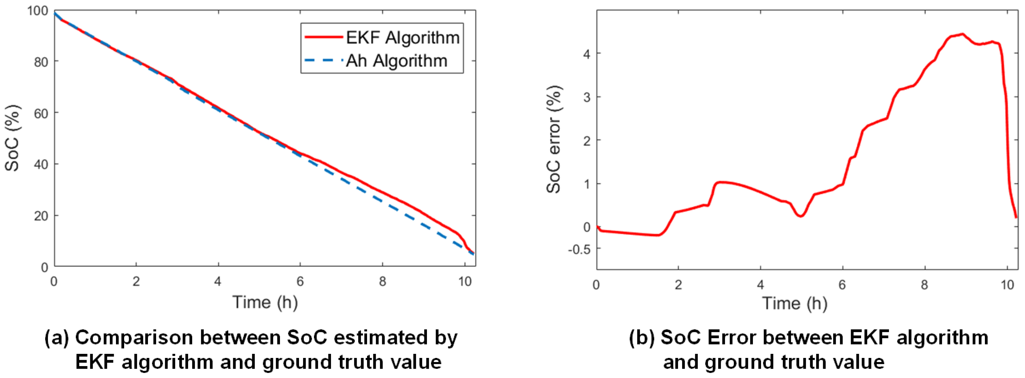
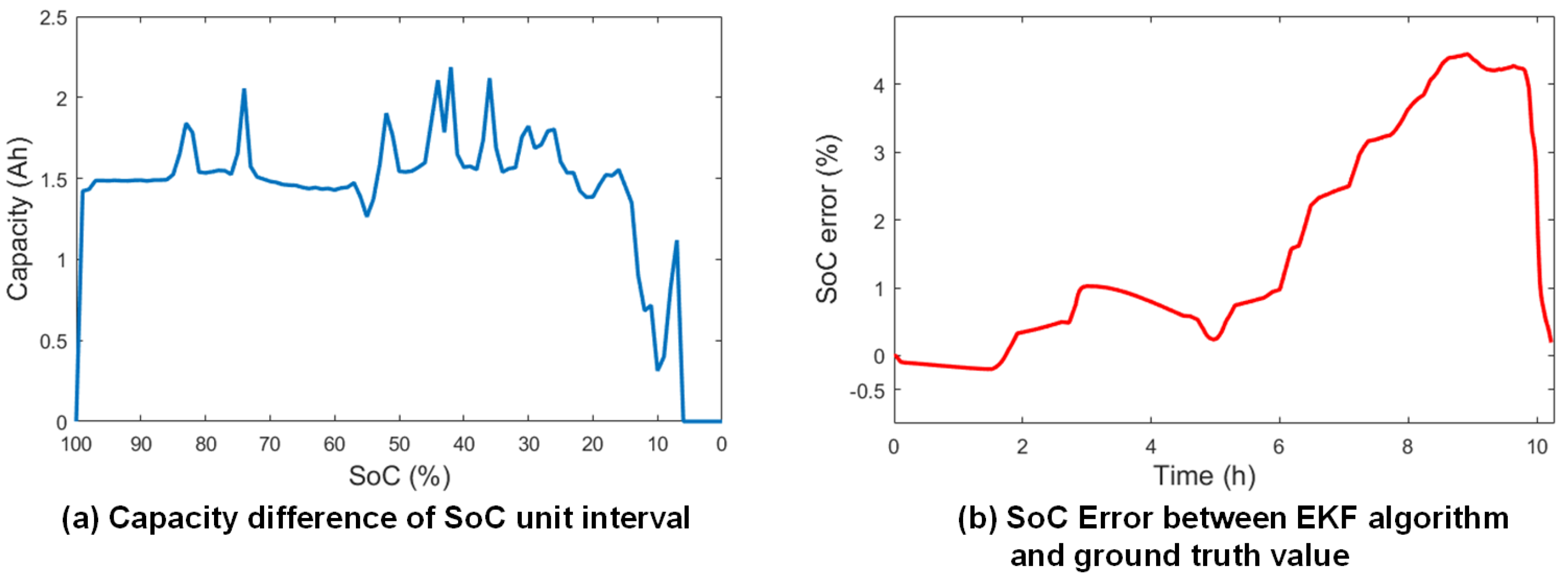
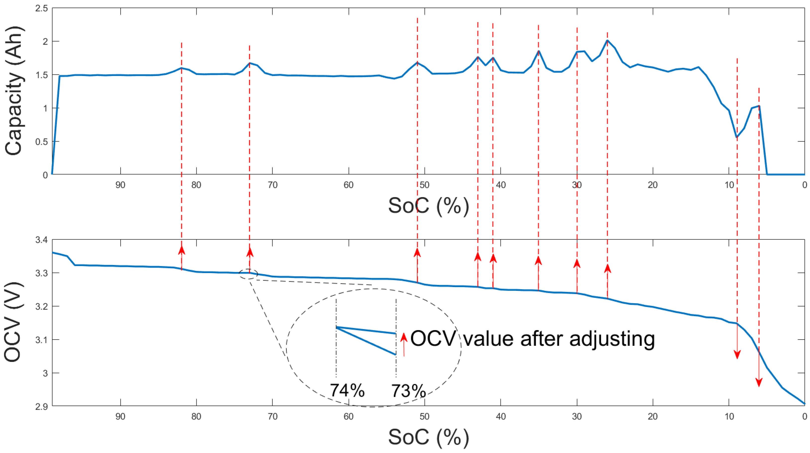
The SoC error indicates the cumulative error, while the capacity difference indicates the actual error between adjacent SoC points. Figure 3 shows the difference and relationship between CDS criterion and SoC error. In fact, the capacity difference shown in Figure 3a is proportional to the derivative of the SoC error shown in Figure 3b.

Figure 3. Comparison between capacity difference and SoC error: (a) Capacity difference of SoC unit interval; (b) SoC Error between EKF and the ground truth.

(2)

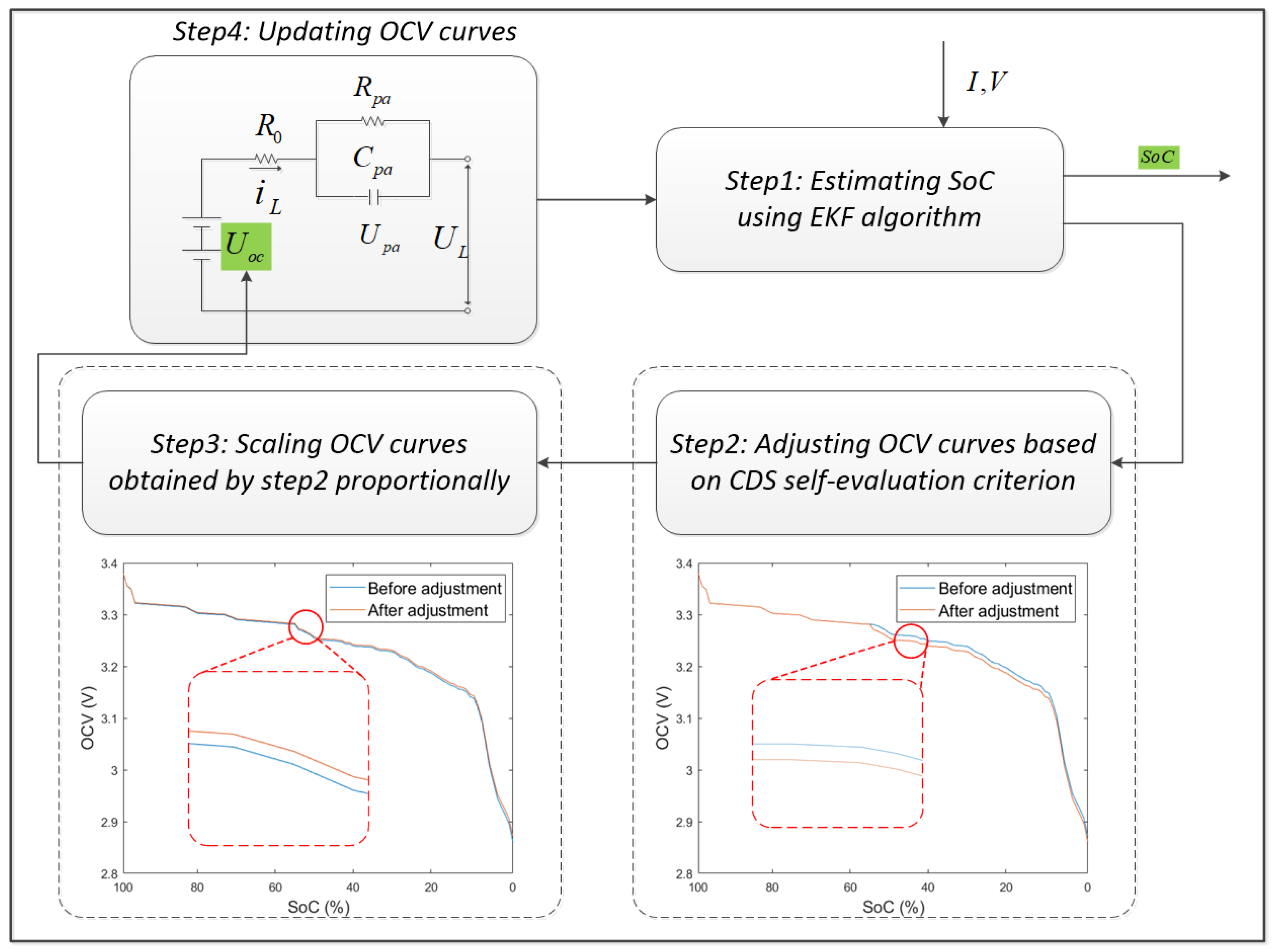
The self-evaluation criterion can be integrated into any EKF-based SoC estimation algorithm where the OCV curve is adjusted adaptively. Therefore, online evaluation of SoC estimation and adjustment of the OCV curve can be achieved.

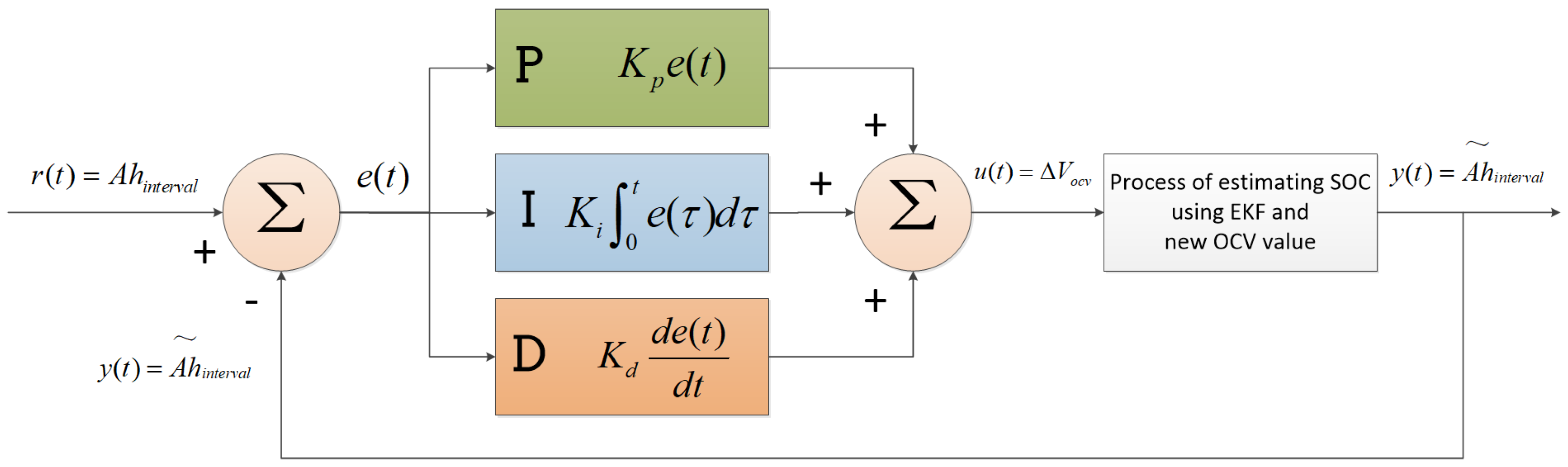
3.3. The Framework of EKF with the CDS Self-Evaluation Criterion

In this section, we propose a novel framework which combines CDS self-evaluation criterion and EKF. The framework consists of four steps: (1) Estimating SoC using EKF; (2) adjusting OCV values based on the CDS self-evaluation criterion; (3) scaling the OCV values proportionally; (4) updating the OCV values for the next SoC estimation. The flowchart of the framework is illustrated in Figure 4.

Figure 4. Flowchart of EKF with CDS self-evaluation criterion.

Step 1 is to estimate SoC using EKF. The interval of SoC is $1\%$. If the change of SoC is greater than $1\%$, go to Step 2.

Step 2 is adjusting OCV values based on the CDS self-evaluation criterion. While using EKF to estimate SoC, the coulomb counting method is used to record the capacity value in each SoC unit interval.

This capacity value is defined as ${\widetilde{Ah}}_{interval}$, where the value of interval is $1\%$. On the other hand, it is assumed that the actual capacity of the battery is known, which is 150 Ah in this experiment. Thus, the actual capacity value in the $1\%$ SoC interval should be 1.5 Ah. This capacity value is defined as ${Ah}_{interval}$. Since there are errors of parameters of the battery model, ${\widetilde{Ah}}_{interval}$ is different with ${Ah}_{interval}$ in each SoC unit interval. We thus define the error of the capacity difference in SoC unit interval as:

$$Er{r}_{interval}=\frac{{\widetilde{Ah}}_{interval}-{Ah}_{interval}}{{Ah}_{interval}}$$

(5)

If ${\widetilde{Ah}}_{interval}>{Ah}_{interval}$, the OCV value at the end of the SoC interval should be increased, which means the OCV difference between the two ends of the SoC interval is reduced. When the EKF is applied to estimate the SoC interval again, ${\widetilde{Ah}}_{interval}$ will become closer to the ground truth value ${Ah}_{interval}$. For example, in Figure 5, ${\widetilde{Ah}}_{[74\%,73\%]}>{Ah}_{[74\%,73\%]}$. We therefore increase the OCV value at $73\%$ point, thus reducing voltage difference between the OCV value at $74\%$ and $73\%$. When the EKF is applied to estimate this SoC interval again, ${\widetilde{Ah}}_{[74\%,73\%]}$ is closer to ${Ah}_{[74\%,73\%]}$. On the contrary, when ${\widetilde{Ah}}_{interval}<{Ah}_{interval}$, the OCV value at the end of the SoC interval should be reduced. Through this adjustment, we can make ${\widetilde{Ah}}_{interval}$ closer to ${Ah}_{interval}$, and minimize $Er{r}_{interval}$. The adjusted value is defined as $\Delta V_{OCV}$.

Figure 5. The OCV curve is adjusted based on the difference of capacity.

Moreover, the OCV curve should be monotonous. That is, the OCV curve should decrease with the decrease in SoC. However, it is possible to break the monotonicity of the OCV curve by applying $\Delta V_{OCV}$ merely on OCV values of the current SoC. For example, the OCV value at $73\%$ point should be reduced if ${\widetilde{Ah}}_{[74\%,73\%]}<{Ah}_{[74\%,73\%]}$. Thus, the new OCV value at $73\%$ point will be lower than the OCV value at $72\%$ point. To keep the OCV curve monotonous, we apply the adjustment value $\Delta V_{OCV}$ on all OCV values of the current and subsequent SoC.

Step 3 is to scale the OCV curve obtained by step 2 proportionally. Applying $\Delta V_{OCV}$ on all OCV values of the current and the subsequent SoC will make the voltage range of the new OCV curve different from the previous one. After several iterations of the OCV estimation, the accumulation of difference will cause the new OCV curve to deviate seriously from the correct OCV curve. To keep the voltage range of the new OCV curve constant, which means to keep the voltages at $0\%$ and $100\%$ constant, we scale the OCV curve obtained by step 2 proportionally.

Step 4 is to update the OCV curve. The new OCV curve is used in the next SoC estimation.

The steps of the framework are described in Algorithm 2.

Furthermore, to make the system more stable and meet the convergence speed requirements of the system in real applications, a Proportional–Integral–Derivative (PID) controller is incorporated into the framework to adjust the parameter $\Delta V_{OCV}$ in step 2. The PID controller is shown in Figure 6, where $r\left(t\right)$ is the setpoint value (${Ah}_{interval}$) and $y\left(t\right)$ is the measurement value (${\widetilde{Ah}}_{interval}$). The difference between these two values ($e\left(t\right)$) is used as the input to the PID controller. The output of the PID controller ($u\left(t\right)$) is the adjusted value of the OCV ($\Delta V_{OCV}$). Finally, these adjusted values are used to form a new OCV curve. The new OCV curve is then used to estimate the SoC in EKF, where a new ${\widetilde{Ah}}_{interval}$ is obtained and returned as the measurement value.

Figure 6. PID controller for adjustment of $\Delta V_{OCV}$.

Algorithm 2 EKF Algorithm with CDS self-evaluation criterion

01: input: $So{C}_{old}=So{C}_{intial}$ 02: for i = 1 to N do 03:  Step 1: Estimate SoC using EKF 04:    if ($|So{C}_{new}-So{C}_{old}|>=1$) 05:     goto Step 2 06:    end if 07:  Step 2: Adjust OCV values based on CDS self-evaluation criterion 08:    $Er{r}_{interval}=\frac{{\widetilde{Ah}}_{interval}-{Ah}_{interval}}{{Ah}_{interval}}$ 09:    if ($|Er{r}_{interval}|>1\%$) 09:     Calculate adjustment voltage of OCV, $\Delta V_{OCV}$, according to ${Err}_{interval}$ 11:     Adjust current and subsequent OCV values to get $V_{SoC=i\%}^{new}$ 12:     for i = ${SoC}_{new}$ to 0 do 13:      $V_{SoC=i\%}^{new}=V_{SoC=i\%}^{old}+\Delta V_{OCV}$ 14:     end for 15:    else 16:     continue 17:    end if 18:  Step 3: Scale the OCV curve obtained by step 2 proportionally 19:    for i = 100 to 0 do 20:     $V_{diff}=V_{SoC=100\%}^{old}-V_{SoC=0\%}^{old}$ 21:     $\Delta ratio=\left(V_{diff}\right)/(V_{diff}+\Delta V_{OCV})$ 22:     $V_{SoC=i\%}^{newnew}=(V_{SoC=100\%}^{old}-(V_{SoC=100\%}^{old}-V_{SoC=i\%}^{new})\ast \Delta ratio$ 23:    end for 24:  Step 4: Update the OCV curve 25:    for i = 100 to 0 do 26:     $V_{SoC=i\%}^{old}=V_{SoC=i\%}^{newnew}$ 27:    end for 28: end for

3.4. Memory Consumption Analysis

Considering the limited system resources of traditional BMS, to enable BMS to achieve online OCV estimation, the proposed framework is then optimized to reduce the additional requirements for system resources such as memory consumption and CPU utilization rate. The additional memory requirements are as follows:

(1)

A variable OCV curve requires an additional 202 bytes of memory for each cell in series.

(2)

The actual capacity ${\widetilde{Ah}}_{interval}$ in the $1\%$ SoC interval requires 2 bytes of memory for each cell in the series. This value is used as the input for the adjustment of the OCV curve. If we need to observe all ${\widetilde{Ah}}_{interval}$ in the full SoC intervals, 200 bytes are necessary to store the data.

(3)

If PID is used to accelerate the convergence speed of the method, 4 floats are needed to store the temporary variables.

In terms of memory consumption, each cell in the series needs additional memory of 418 bytes ($101\ast 2+100\ast 2+4\ast 4=418$). If the ESS system is constructed by 250 cells in the series, the method requires about 105K bytes of memory. In terms of the CPU utilization rate, since each calculation will only happen at the time that SoC changes by $1\%$, the increase in the CPU utilization rate is negligible. Therefore, the consumption is acceptable for traditional BMS with limited system resources.

4. Experimental Results and Analysis

We evaluate the effectiveness of the proposed EKF with CDS self-evaluation on an ESS scenario experiment. The OCV curve and DV curve are obtained after 200 discharge iterations in the proposed algorithm framework. Meanwhile, we use the pseudo-OCV test method to obtain the OCV curve and DV curve in the laboratory environment. The OCV curve and DV curve are compared with the estimated values to verify the effectiveness of the proposed method.

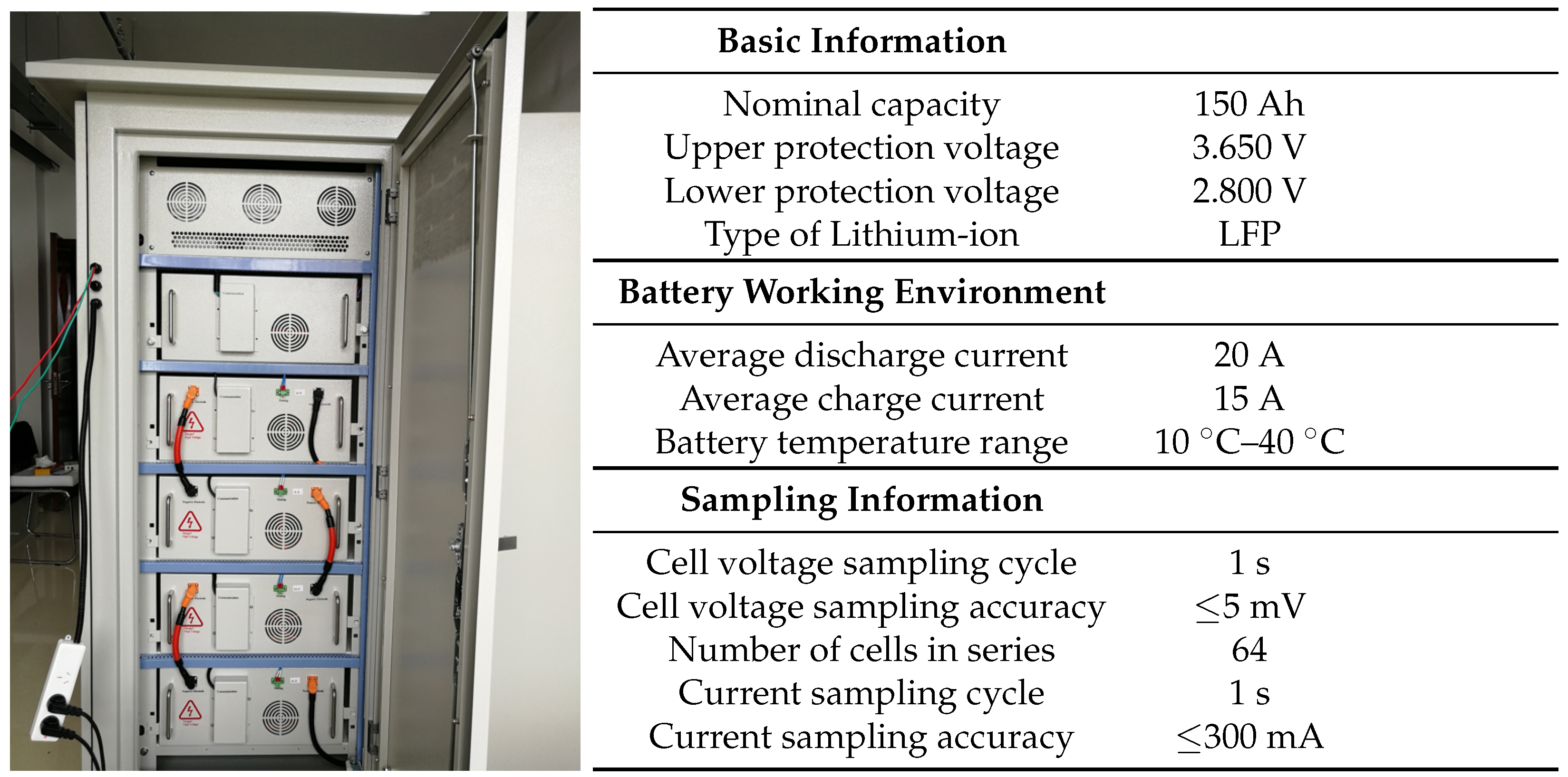
4.1. Experimental Environment

The ESS is equipped with LFP batteries. Figure 7 summarizes the basic parameters of the battery, information of the environment, sampling information, etc. All of the original data of the battery are obtained from BMS on ESS, which are uploaded to a personal computer (PC) through a controller area network (CAN) bus and saved in the database.

Figure 7. Basic information of LFP batteries on an experimental ESS.

These original data include the voltage, current, temperature, SoC and the internal resistance of the system. The voltages of the cells in series are sampled by LTC6803-4 multi-series battery monitoring IC, where the sampling period is 1s and the measurement accuracy is $\pm 5$ mv. The current is sampled by, shunt where the sampling period is 1 s and the measurement accuracy is $\pm 300$ mA. The temperature sampling is completed by LTC6803-4, where the sampling period is 1s and the measurement accuracy is $\pm 1{}^{\circ }\mathrm{C}$. The original SoC and internal resistance estimation data come from BMS. BMS uses EKF to estimate the SoC and internal resistance of each cell in series.

The battery of ESS is fully charged firstly. The first cell is selected as the experimental object. The first cell is charged to $99\%$ SoC and then discharged to about $6\%$ SoC. The battery data come from the actual ESS. Since one cell in the ESS is fully charged, the first cell can not be fully charged due to the barrel effect, which results in the termination of the charging process. Moreover, the ESS reserves about $6\%$ capacity for longer battery life. Figure 8a shows the current change while the ESS is running. Figure 8b shows the voltage change of the first cell. The change in the temperature of the cell is $29{}^{\circ }\mathrm{C}$ to $31{}^{\circ }\mathrm{C}$.

Figure 8. The current and the voltage of the 1st cell while ESS is running: (a) Current. (b) The voltage of the 1st cell.

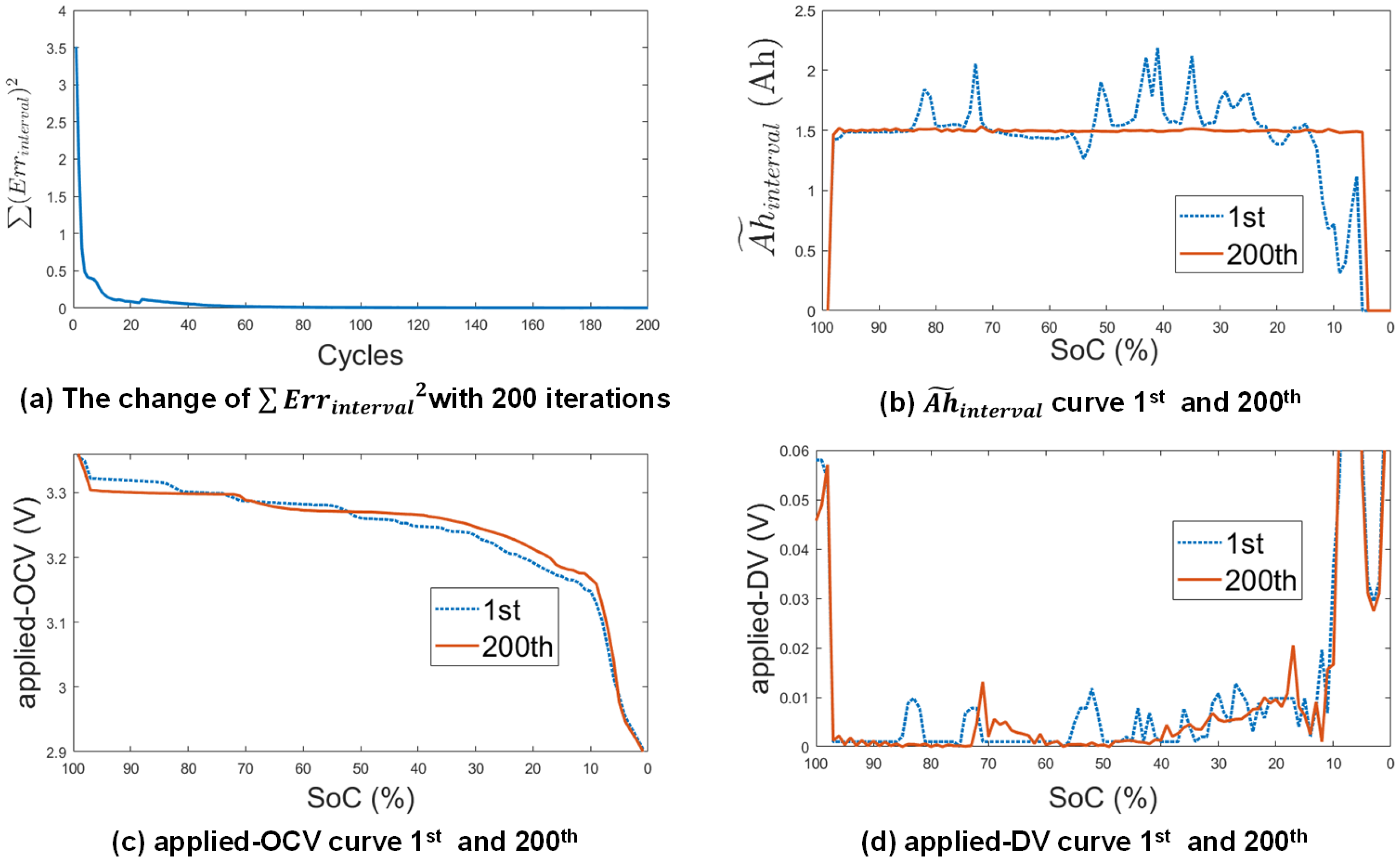
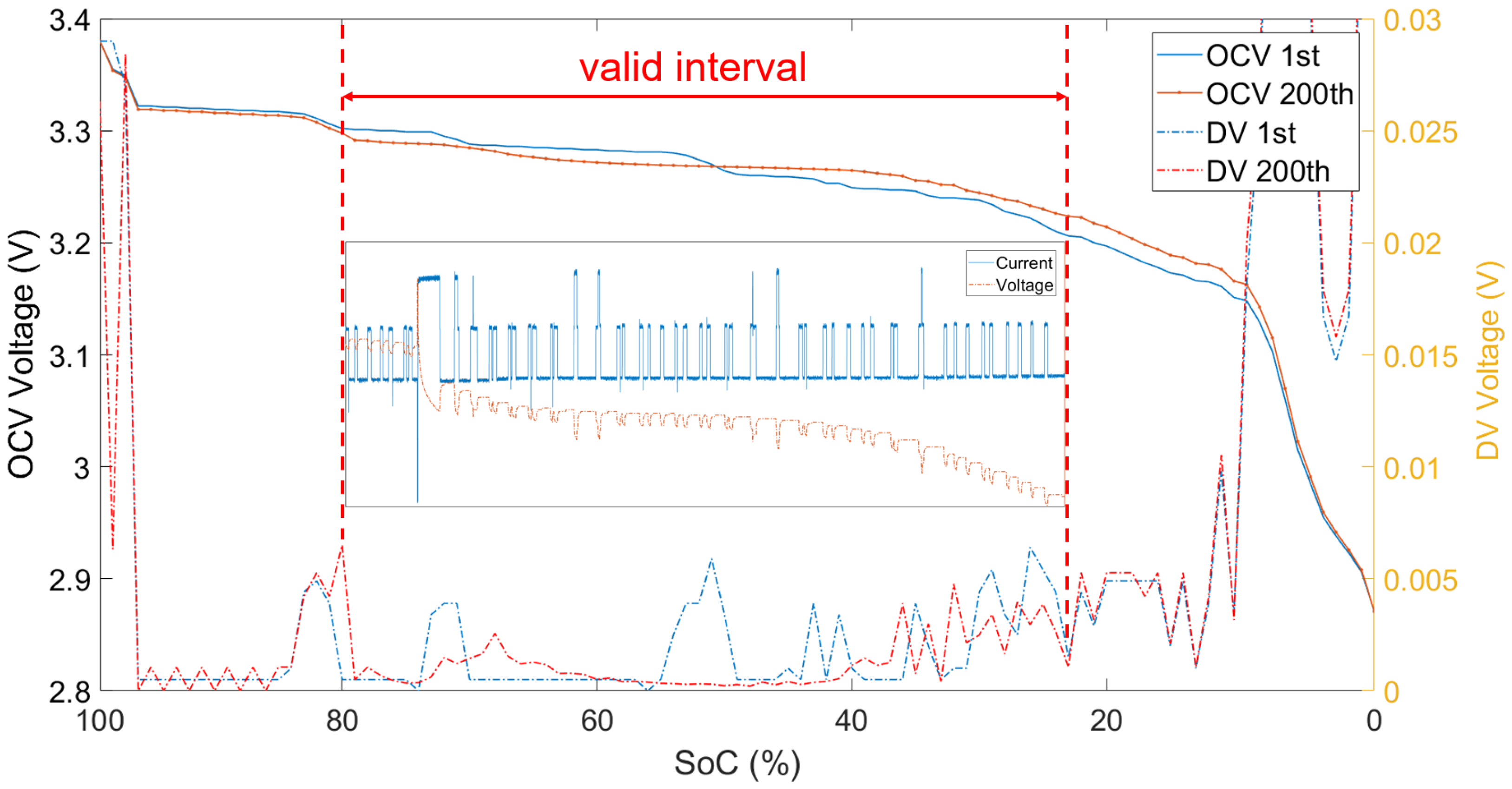
4.2. Experimental Results after 200 Iterations

In this experiment, 200 iterations of discharging processes are completed. After each iteration, according to Equation (5), we get $\sum {\left(Er{r}_{interval}\right)}^2$ of all effective SoC intervals. The changing process of $\sum {\left(Er{r}_{interval}\right)}^2$ is shown in the Figure 9a. Through the value of $\sum {\left(Er{r}_{interval}\right)}^2$, we can observe the convergence of the proposed method. Figure 9b shows the comparative results of the first and the last ${\widetilde{Ah}}_{interval}$ curve. After the 200th iteration, the values of ${\widetilde{Ah}}_{interval}$ on all valid SoC intervals are more closer to the ground truth value 1.5 Ah of ${Ah}_{interval}$.

Figure 9. The change process of ${\widetilde{Ah}}_{interval}$/OCV curve/DV curve from 1st to 200th: (a) The change in $\sum {\left(Er{r}_{interval}\right)}^2$ with 200 iterations; (b) 1st and 200th ${\widetilde{Ah}}_{interval}$ curve; (c) 1st and 200th applied-OCV curve; (d) 1st and 200th applied-DV curve.

In our method, the OCV curve is strongly related to the scenario in which the battery is used. It is also related to the SoC estimation algorithms used, the battery model and the model parameters. Therefore, we refer to the OCV curve obtained by our method as the applied-OCV curve to distinguish it from OCV curves obtained from offline approaches, e.g., a pseudo-OCV curve. The objective of offline approaches such as GITT or pseudo-OCV is to lower the electrode polarization, reduce the kinetic contributions, ohmic heat generation and the voltage hysteresis. That is, GITT and pseudo-OCV approaches need to minimize the impact of the external input current on the battery. However, our applied-OCV curve is learned from the running environment. The impact of the current will be further added onto the applied-OCV curve.

Although applied-OCV curve is not a strict OCV curve, the shape of the applied-OCV curve is very consistent with the OCV curve achieved by GITT or a pseudo-OCV test approach. Therefore, the applied-OCV still indicates the characteristics of the batteries, such as the number of phases, the phase transitions and the change in the amount of lithium intercalated in any given phase. These characteristics can be reflected in the IC-DV curves of the battery, which indicates the degradation process of the battery. Figure 9c shows the comparison results of the first applied-OCV curve and the last applied-OCV curve.

IC-DV curves are considered to be the most effective tool for battery degradation analysis [43]. IC-DV curves are usually derived from OCV in an offline manner. With an accurate and finer applied-OCV curve obtained in our approach, more accurate IC-DV curves can also be obtained online. Since the capacity value in each SoC interval tends to be consistent, the DV curve can be easily obtained from the derivative of the applied-OCV curve. We refer to the DV curve obtained using our method as the applied-DV curve. Figure 9d shows the comparison results of the first and last applied-DV curve.

Since OCV curve is an important parameter for EKF-based SoC estimation, a more accurate applied-OCV is beneficial for improving the accuracy of SoC estimation. Figure 10 shows the result of SoC estimation leveraging EKF with CDS criterion. Compared with the SoC estimation result by EKF in Figure 2, the RMSE of SoC estimation is reduced from $2.23\%$ to $0.07\%$. The maximum error of SoC estimation is reduced from $4.44\%$ to $0.24\%$.

Figure 10. Comparison between SoC estimated by EKF with CDS algorithm and the ground truth (SoC calculated by coulomb counting method): (a) Comparison between SoC estimated by EKF with CDS and the ground truth; (b) SoC error between EKF with CDS and the ground truth.

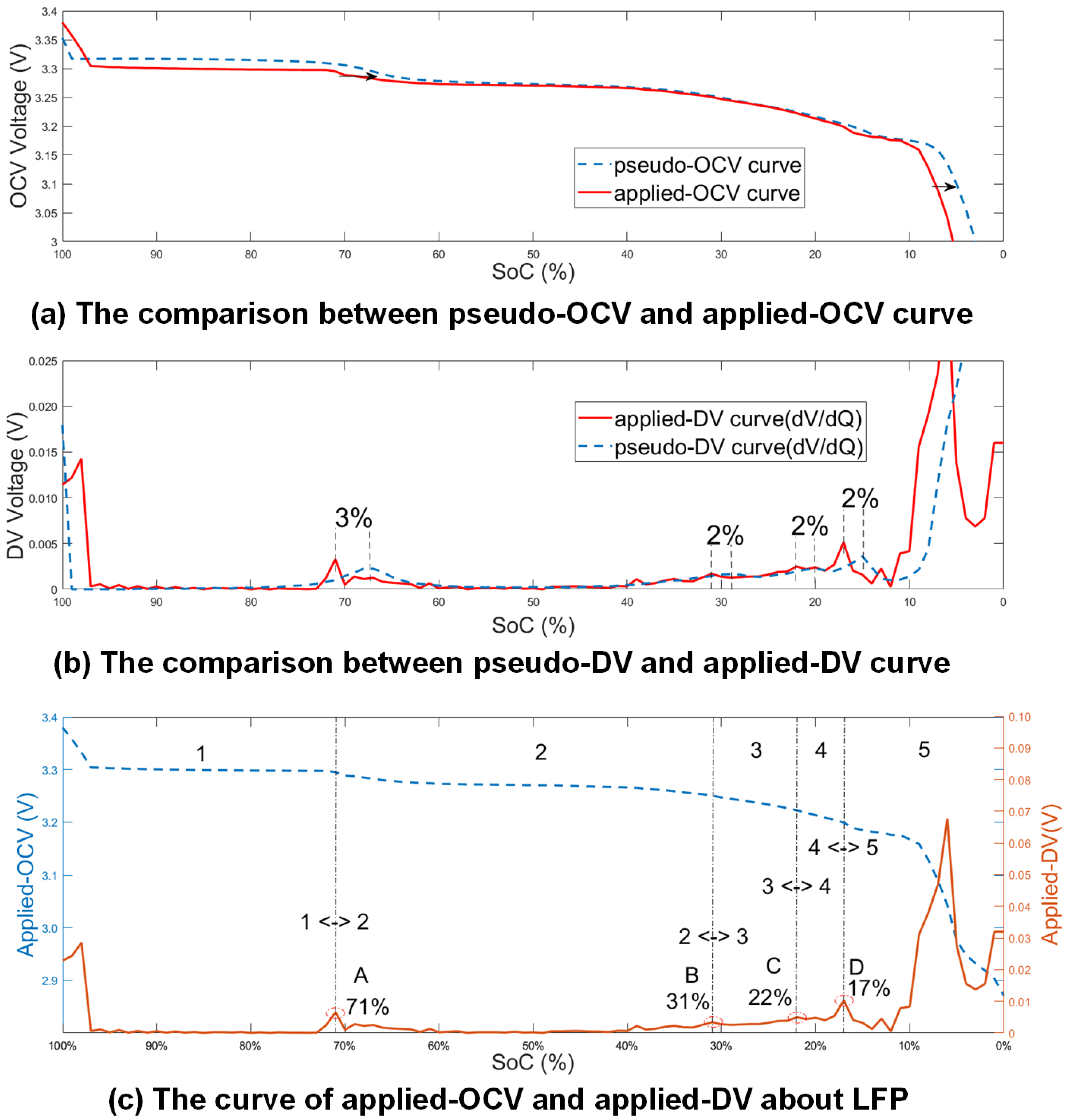
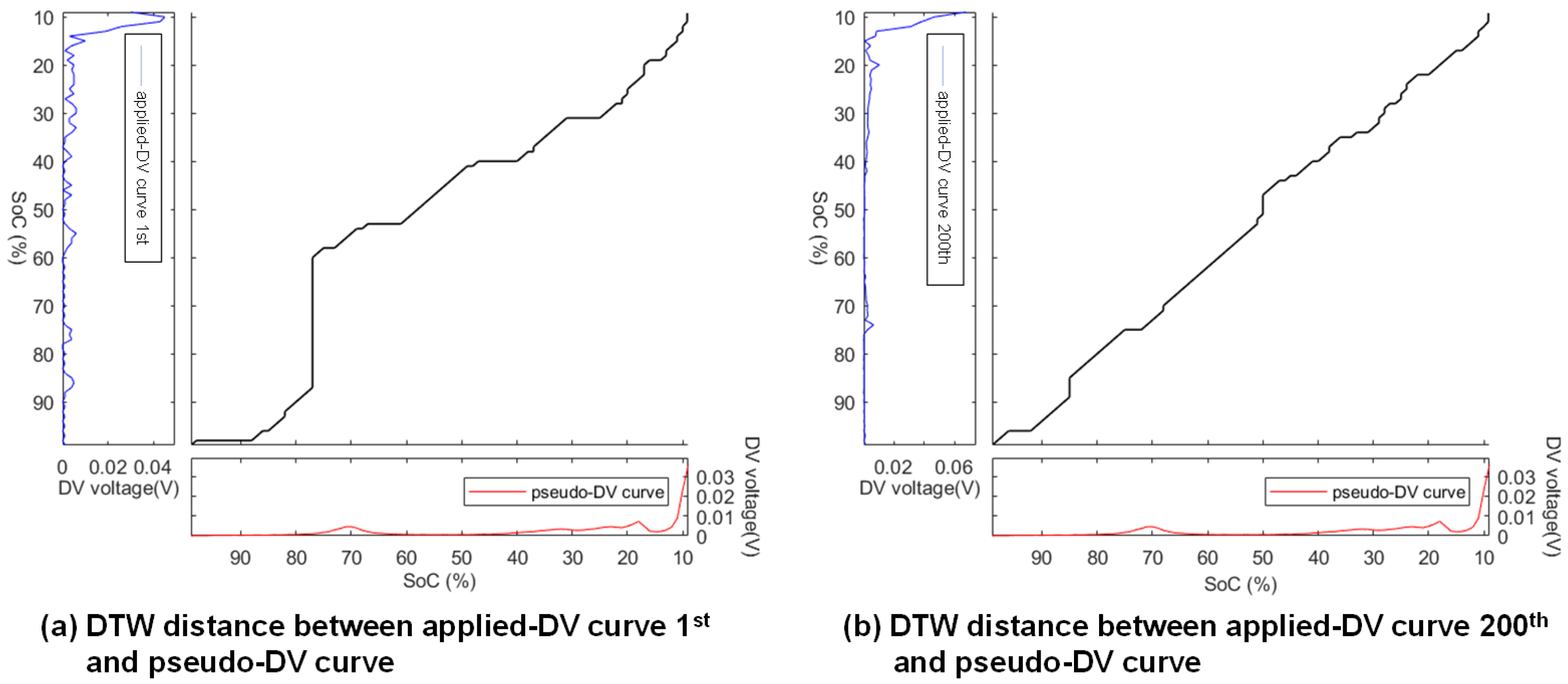
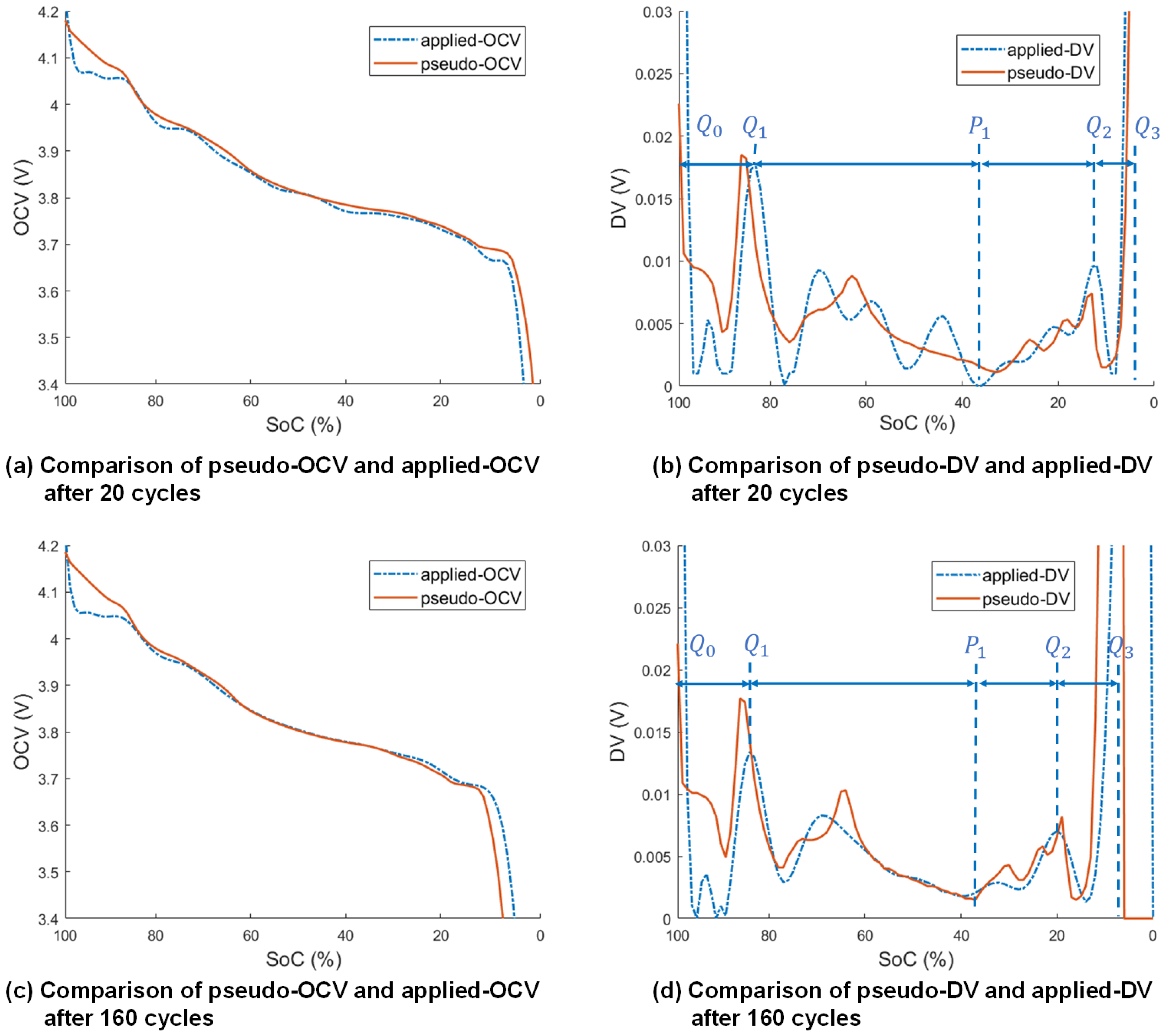
4.3. Comparison with the Pseudo Test Method

The pseudo-OCV of the LFP battery in ESS is obtained by discharging a single battery with $C/25$ under the constant temperature of $20{}^{\circ }\mathrm{C}$ in the laboratory. Figure 11a shows the comparison between the pseudo-OCV curve and the applied-OCV curve. From Figure 11a, it can be observed that although the shapes of the two curves are very similar, there are some deviations since the applied-OCV is obtained from the actual ESS system. To ensure the battery cycle life in the actual system, the upper and lower limits of the voltage protection range will be more narrow than the upper and lower voltage protection range when measuring the pseudo-OCV curve, which causes the SoC to have an offset of $2\%$. Moving the applied-OCV curve by $2\%$ in the descending direction of SoC, the applied-OCV curve is more similar to the pseudo-OCV curve. Figure 11b compares the pseudo-DV curve and the applied-DV curve. It can be seen that the two curves are very similar. Due to different protection voltage ranges between the real scene and the experimental scene, there is a phase offset of about $2\%$ between the two curves. A more detailed description of the applied-OCV curve and the applied-DV curve can be observed in Figure 11c. As described in [43], the 4 characteristic peaks are located at $71\%$, $31\%$, $22\%$ and $17\%$ SoC, respectively, representing non-stoichiometry in the single-phase regions (solid line), as denoted by A to D. The valleys between peaks represent the graphite staging phenomena, as denoted by 1 to 5. The peaks of the applied-DV curve are consistent with the peaks of the pseudo-DV curve.

Figure 11. The comparison between pseudo-OCV and applied-OCV.

Dynamic Time Warping (DTW) is widely used to measure the similarity between two temporal sequences. Especially for two temporal sequences of different lengths, DTW can “warp” the time axis of one (or both) sequences to achieve a better alignment. DTW first builds a $m\times n$ distance matrix (typically the Euclidean distance) between any two points on two temporal sequences. Then, a continuous warping path, which is composed of a set of adjacent matrix elements, is obtained to define the mapping between the sequences. Finally, the sum of all the distance values on this warping path is used to evaluate the similarity between the two sequences [44,45,46]. We use DTW to measure the similarity between the pseudo-DV curve and the applied-DV curve. Figure 12a shows the warping path and the distance between the initial applied-DV curve and the pseudo-DV curve. The DTW distance is $0.126$. Figure 12b shows the warping path and distance between the 200th applied-DV curve and the pseudo-DV curve. The DTW distance is decreased to $0.0977$. The small DTW distance indicates that the applied-DV curve obtained by our method is closer to the pseudo-DV curve.

Figure 12. DTW warping paths and distances between pseudo-DV curve and applied-DV curve.

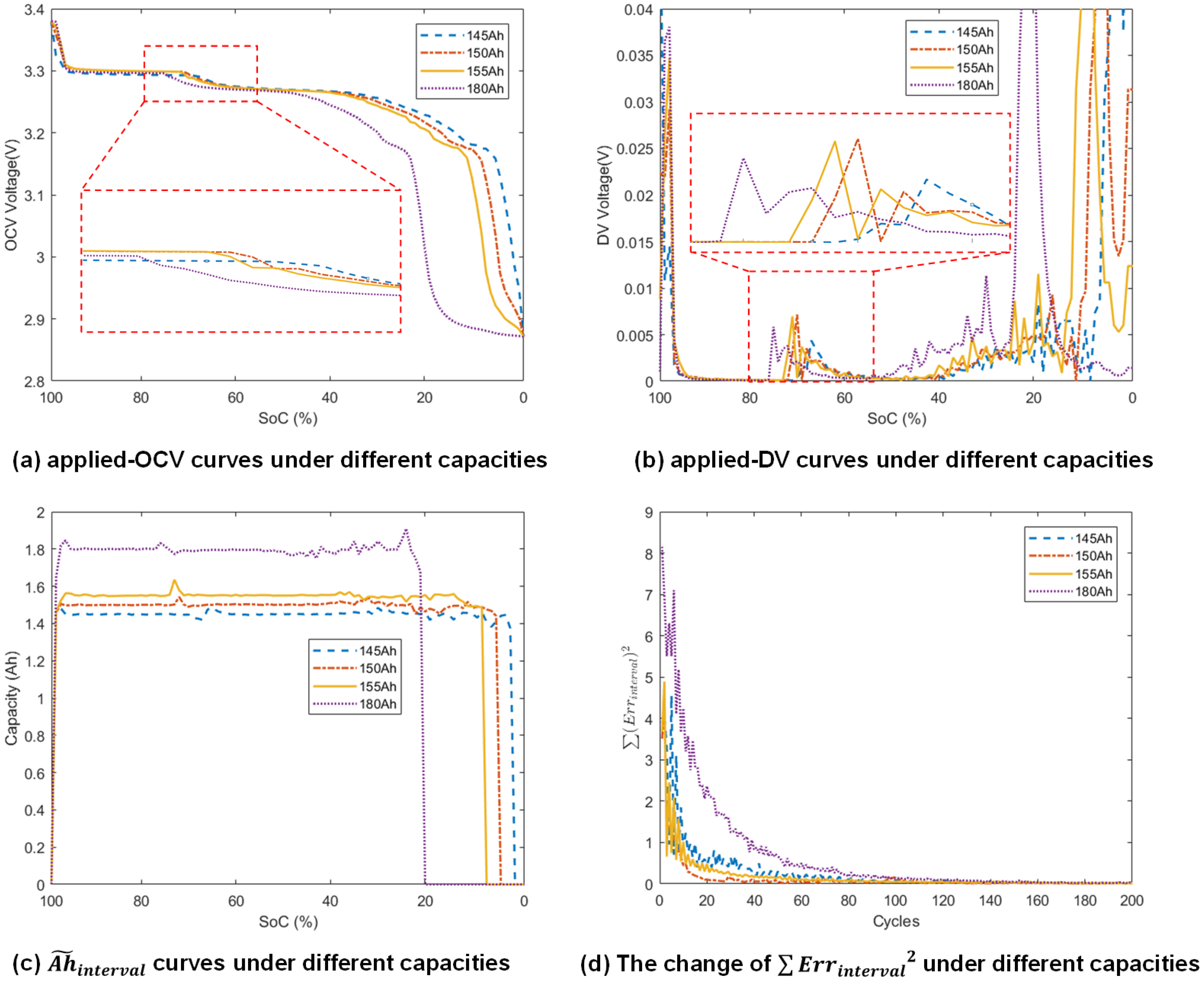
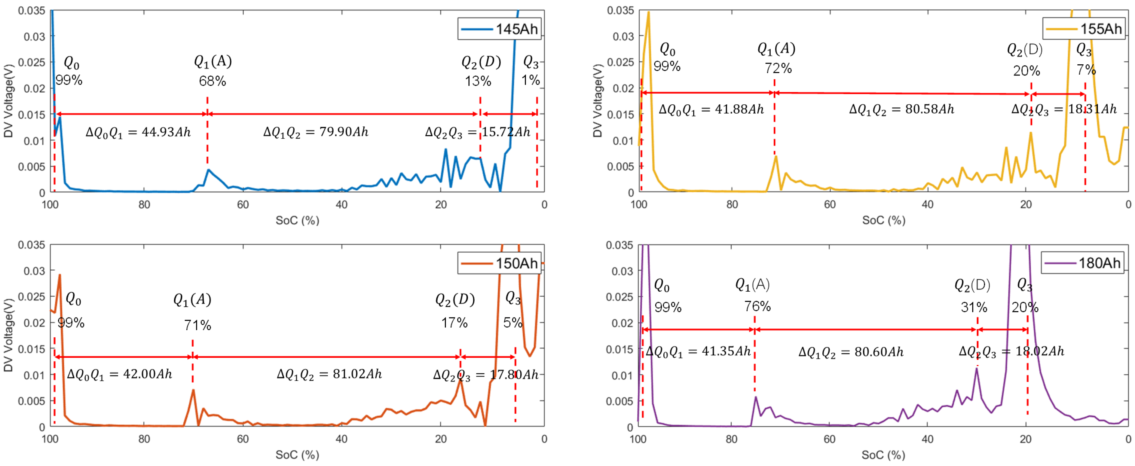
4.4. Experimental Results with Different Battery Capacities

In our method, battery capacity is an important parameter. We assume that the battery capacity is known in this paper. Accurate battery capacity estimation plays a critical role in ensuring the safety and preventing catastrophic hazards. Since the battery capacity will inevitably decrease with the aging of the battery, it is difficult to estimate accurate battery capacity due to the varying current and partial cycle.

The battery capacity estimation can be generally classified into three categories: model-based, IC-DV curves-based, and machine-learning-based. Furthermore, a convolutional neural network (CNN) is applied to estimate the battery capacity using the measured voltage, current and the calculated cumulative capacity. The overall RMSEs are less than $2\%$ on the NASA dataset [47].

The initial battery capacity used in our experiment is 150 Ah. Using the aforementioned methods, the overall RMSEs of the battery capacity estimation are less than $2\%$, which means that the capacity value may change from 147 Ah to 153 Ah. Based on the different battery capacities, we simulate the reduction of battery capacity caused by aging and analyze the influence of battery capacity on our method.

To facilitate comparison, four battery capacities—145 Ah, 150 Ah, 155 Ah and 180 Ah, respectively—are selected as given capacity values to complete the online OCV estimation. Figure 13a shows the estimated results of the OCV. Figure 13b shows the estimated results of the DV. It can be seen that there are obvious differences in the estimated OCV under different battery capacities. However, the basic shapes of the these OCV curves are highly consistent. Figure 13c shows the values of ${\widetilde{Ah}}_{interval}$ on a full SoC range after the 200th iteration based on different battery capacities. The capacity value in the unit SoC interval ${\widetilde{Ah}}_{interval}$ converges to the given capacity value ${Ah}_{interval}$. In particular, when the given capacity value is 180 Ah, ${\widetilde{Ah}}_{interval}$ is 0 on SoC in the interval ranging from $20\%$ to $0\%$. This is because the actual capacity of the battery has been exhausted on SoC ranging from $100\%$ to $20\%$. Figure 13d shows the convergence rate of the method based on different battery capacities. A change in the battery capacity will not affect the convergence of our method.

Figure 13. Experimental results under different battery capacities.

In the DV curve, the features related to the characteristic peaks describe the different paths and degrees of battery degradation. For the LFP battery, two characteristic peaks $Q_1\left(A\right)$ and $Q_1\left(D\right)$ are more significant than other characteristic peaks, such as peaks B and C in Figure 11c. These two characteristic peaks divide the voltage profile into three plateaus, which are indicated by three valleys in the DV curve. The lengths and positions of these three plateaus in the voltage profiles are directly influenced by the aging mechanisms which take place during the lifetime of the battery.

As shown in Figure 14, based on the different given battery capacities, the features related to the two peaks are extracted, including the capacity (Ah) from the beginning discharge point $Q_0$ to peak $Q_1$ ($\Delta Q_0{Q}_1$), the capacity (Ah) between peaks $Q_1$ and $Q_2$ ($\Delta Q_1{Q}_2$), the capacity (Ah) from peak $Q_2$ to the ending discharge point $Q_3$ ($\Delta Q_2{Q}_3$) and the OCV values corresponding to peaks $Q_1$ and $Q_2$. The values of the features are shown in Table 3.

Figure 14. Experimental results under different battery capacities.

Table 3. Extracted features from the applied-DV curve based on different given battery capacities.

Given Capacity	$\Delta {\mathit{Q}}_0{\mathit{Q}}_1$ (Ah)	$\Delta {\mathit{Q}}_1{\mathit{Q}}_2$ (Ah)	$\Delta {\mathit{Q}}_2{\mathit{Q}}_3$ (Ah)	${\mathit{U}}_{\mathbf{oc}}$ at ${\mathit{Q}}_1$ (V)	${\mathit{U}}_{\mathbf{oc}}$ at ${\mathit{Q}}_2$ (V)
145 Ah	44.93	79.90	15.72	3.2897	3.1898
150 Ah	42.00	81.02	17.80	3.2952	3.1973
155 Ah	41.88	80.58	18.31	3.2956	3.2018
180 Ah	41.35	80.60	18.02	3.2959	3.2014

Different given battery capacities have small effects on the features related to peaks $Q_1$ and $Q_2$. That is to say, the errors in battery capacity estimation will not affect the accuracy of the features extracted from the applied-DV/OCV curve in our method. These features can be leveraged to evaluate the paths and degrees of battery degradation, and even to verify the accuracy of the battery capacity estimation.

4.5. Experimental Results with Partial Cycle

In practical use, the battery often cannot carry out a full charging or discharging cycle. In this case, our method can only estimate the OCV curve in the valid interval. The experiment is designed to simulate a situation with a partial cycle. The data are chosen from the full data of the cycle. We set the initial SoC to $80\%$ and the battery capacity to 150 Ah. These data form a valid interval. Figure 15 shows the results. It can be seen that the proposed method is able to estimate the OCV curve and the DV curve in the valid interval. Different initial SoC values affect the correlation of the SoC-OCV curve. The incorrect initial SoC values will make the SoC-OCV curve shift. However, the shapes of the SoC-OCV curve are mostly retained. Different given battery capacities also affect the correlation of the SoC-OCV curve. An incorrect battery capacity will scale the SoC-OCV curve. It has little effect on the features extracted from the OCV or DV curve, as discussed in Section 4.4.

Figure 15. Experimental results with partial cycle.

4.6. Experimental Results with Aged Battery

To evaluate the effectiveness of the proposed method for an aged battery, a set of experimental charging and discharging profiles based on lithium polymer battery is designed, which includes pseudo-OCV measurement on different cycles, a federal urban driving schedule (FUDS) test for our OCV estimation method, and a set of cycle tests to simulate the battery aging. The steps of experimental profiles are as follows: Step 1: The charge and discharge OCV of the battery are obtained using a pseudo test method with constant charge and discharge current of 1A (1/20C). These pseudo-OCV/DV curves are compared with the applied-OCV/DV curves estimated below. Step 2: An experiment based on the dynamic stress test FUDS is designed. The battery is charged to 4.2 V with constant current of 1 A. It is then discharged to 2.5 V based on FUDS. The sampling periods of voltage and current are 1s. These data are used to estimate the applied-OCV/DV curve. The reason why we choose FUDS is that we want to verify the effectiveness of the proposed method in case of a violent current profile. Step 3: A set of 20 charge and discharge cycles (20 A for discharging, 10 A for charging) is completed to simulate battery aging. Part of the experimental data of the above three steps are shown in Figure 16. These steps are repeated until the battery completes the experiment of 160 cycles.

Figure 16. The three steps of experimental charging and discharging profiles.

To compare the changes in the applied-OCV/DV curves with battery aging, the battery capacity used in applied-OCV/DV estimation is set to a constant value of 22 Ah. If the actual battery capacity decreases with cycles, the applied-OCV/DV curves will indicate a trend of scale and shift to the left. Figure 17 shows the applied-OCV/DV curves under different cycles.

Figure 17. Applied-OCV/DV curves under different cycles.

A locally enlarged applied-DV shows the process of battery-capacity reduction. Figure 18 shows two characteristic peaks of the applied-DV curve; one peak, $Q_1$, is close to $80\%$ SoC, and another peak, $Q_2$, is close to $20\%$ SoC.

Figure 18. Partial applied-DV curves around $80\%$ and $20\%$ SoC.

Five applied-DV curves with different cycles are analyzed. Since the formation of solid–electrolyte interphase (SEI) happens within the first few cycles, the battery capacity at the 20th cycle is higher than that on the 1st cycle. The $Q_2$ of the 20th cycle shifts to the right compared with the $Q_2$ of the 1st cycle. With the increase in the number of battery cycles, the battery capacity begins to decrease. Figure 18b shows that the $Q_2$ of the 40th cycle is on the left of the $Q_2$ of the 20th cycle. If the number of the cycle is between 40 and 140, the battery is relatively stable, in which case the capacity remains almost unchanged. From the 160th cycle, the battery capacity decreases more obviously. Figure 18b also shows that the $Q_2$ of the 160th cycle is at the leftmost end of the others. On the other hand, the characteristic peak $Q_1$ is also quite stable in Figure 18a. During 160 cycles, the location of $Q_1$ does not change obviously.

Before each FUDS test, the pseudo-OCV/DV curves are obtained using the discharge current of 1 A (1/20C). Figure 19 shows the pseudo-OCV/DV curves of the battery with different cycles. These curves are compared with the applied-OCV/DV curves at the same number of cycles.

Figure 19. Pseudo-OCV/DV curves under different cycles.

Here, the pseudo-OCV/DV curves and the applied-OCV/DV curves of the 20th and 160th cycle are compared. To facilitate the comparison, we unify the X-coordinate of these curves into SoC, as shown in Figure 20. Due to the relatively drastic current changes in FUDS test, some feature points are no longer obvious on the applied-DV curve, while other feature points show a strong correlation with the corresponding feature points on the pseudo-DV curve. These feature points include characteristic peaks $Q_1$, $Q_2$ and characteristic valley $P_1$, as shown in Figure 20. The features related to $Q_1$, $Q_2$ and $P_1$ are extracted and shown in Table 4. These features include the capacities (Ah) between the characteristic peaks or valley and the OCV values corresponding to $Q_1$, $Q_2$ and $P_1$.

Figure 20. Comparisons of pseudo-OCV/DV curves and applied-OCV/DV curves after 20 and 160 cycles. (a) Comparison of pseudo-OCV and applied-OCV/DV after 20 cycles; (b) comparison of pseudo-DV and applied-DV after 20 cycles; (c) comparison of pseudo-OCV and applied-OCV/DV after 160 cycles; (d) comparison of pseudo-DV and applied-DV after 160 cycles.

Table 4. Extracted features from the applied-DV curves under different cycles.

Cycles	Capacity (Ah)	$\Delta {\mathit{Q}}_0{\mathit{Q}}_1$ (Ah)	$\Delta {\mathit{Q}}_1{\mathit{Q}}_2$ (Ah)	$\Delta {\mathit{Q}}_1{\mathit{P}}_1$ (Ah)	$\Delta {\mathit{P}}_1{\mathit{Q}}_2$ (Ah)	$\Delta {\mathit{Q}}_2{\mathit{Q}}_3$ (Ah)	${\mathit{U}}_{\mathbf{oc}}$ at ${\mathit{Q}}_1$ (V)	${\mathit{U}}_{\mathbf{oc}}$ at ${\mathit{P}}_1$ (V)	${\mathit{U}}_{\mathbf{oc}}$ at ${\mathit{Q}}_2$ (V)
1	21.5478	3.1112	14.5364	12.3360	2.2004	3.9002	4.0230	3.7561	3.7222
20	21.7524	3.5928	15.6278	10.3443	5.2835	2.5318	4.0075	3.7670	3.6858
40	21.6041	3.5821	14.7562	10.3459	4.4103	3.2658	4.0172	3.7743	3.7145
60	21.6994	3.3516	14.9273	10.9834	3.9439	3.4205	4.0307	3.7717	3.7131
80	21.5678	3.3306	14.8856	10.3007	4.5848	3.3516	4.0266	3.7762	3.7088
100	21.5821	3.5871	14.4987	10.3364	4.1623	3.4963	4.0168	3.7732	3.7130
120	21.5697	3.3504	14.7686	10.5885	4.1800	3.4507	4.0326	3.7738	3.7149
140	21.5743	3.3426	14.6787	10.5240	4.1547	3.5531	4.0288	3.7663	3.7082
160	21.0913	3.3342	14.1199	9.7066	4.4133	3.6373	4.0160	3.7789	3.7171

The value of $\Delta Q_0{Q}_1$ remains almost constant during the cycles. $\Delta Q_1{Q}_2$ shows a strong correlation with the capacity of the aged battery. Moreover, $\Delta Q_1{Q}_2$ consists of $\Delta Q_1{P}_1$ and $\Delta P_1{Q}_2$. $\Delta P_1{Q}_2$ tends to remain constant during the cycles. $\Delta Q_1{P}_1$ contributes more to the reduction of battery capacity. The changes of all the features in the applied-DV curve are consistent with those in the pseudo-DV curve.

5. Conclusions

In this paper, we proposed a novel self-evaluation criterion based on the capacity difference of the SoC unit interval for the evaluation of OCV and SoC estimation. Instead of using MAE or RMSE of SoC estimation as the criterion to evaluate the SoC estimation, the proposed criterion uses the capacity difference between two neighboring SoC points. We integrate this criterion into the EKF-based SoC estimation in our framework, where a more accurate and finer OCV curve can be obtained. Meanwhile, a more accurate SoC estimation can also be obtained. The effectiveness of EKF with CDS self-evaluation criterion is evaluated in a typical application scenario, an energy storage system (ESS) using an LFP battery. Extensive experimental results indicate that more accurate and finer OCV and DV can be obtained online, and are quite consistent with the OCV and DV obtained from the pseudo-OCV test approach. Experimental results also indicate that the proposed framework greatly improves the accuracy of SoC estimation at each SoC point where the maximum estimation error of SoC is less than $0.3\%$.

Extensive experiments are carried out to evaluate the effectiveness of the proposed method. Several conclusions can be drawn: in the battery capacity experiment, if the given capacity is changed, the estimated applied-OCV/DV curves will be scaled, but the features extracted from the applied-DV curve, such as the distance between two characteristic peaks, will not change. In the aged battery experiment, applied-OCV/DV curves show a high degree of consistency with pseudo-OCV/DV curves under the same cycles. Under a violent current profile, some characteristic peaks or valleys on applied-DV curves are no longer obvious, while others show significant consistency with those on pseudo-DV curves. The features extracted from these significant peaks or valleys can be leveraged to evaluate the State of Health (SoH) of the battery.

The main contribution of this paper is that a novel algorithm framework is proposed, through which high-precision online OCV estimation can be achieved. The estimation accuracy of the OCV curve can meet the requirement of online battery degradation analysis in future. At the current stage, we assume that the capacity of the battery is known. In future work, we will further integrate the estimation of the capacity of the battery into the framework. More experiments based on NCM & NCA cathode materials for Li-ion batteries will also be completed.

References

1. Birkl, C.R.; Roberts, M.R.; McTurk, E.; Bruce, P.G.; Howey, D.A. Degradation diagnostics for lithium ion cells. J. Power Sources 2017, 341, 373–386. [Google Scholar] [CrossRef]
2. Bloom, I.; Walker, L.K.; Basco, J.K.; Abraham, D.P.; Christophersen, J.P.; Ho, C.D. Differential voltage analyses of high-power lithium-ion cells. 4. Cells containing NMC. J. Power Sources 2010, 195, 877–882. [Google Scholar] [CrossRef]
3. Liu, G.; Ouyang, M.; Lu, L.; Li, J.; Han, X. Online estimation of lithium-ion battery remaining discharge capacity through differential voltage analysis. J. Power Sources 2015, 274, 971–989. [Google Scholar] [CrossRef]
4. Barai, A.; Uddin, K.; Dubarry, M.; Somerville, L.; McGordon, A.; Jennings, P.; Bloom, I. A comparison of methodologies for the non-invasive characterisation of commercial Li-ion cells. Prog. Energy Combust. Sci. 2019, 72, 1–31. [Google Scholar] [CrossRef]
5. Zhu, J.; Darma, M.S.D.; Knapp, M.; Sørensen, D.R.; Heere, M.; Fang, Q.; Wang, X.; Dai, H.; Mereacre, L.; Senyshyn, A.; et al. Investigation of lithium-ion battery degradation mechanisms by combining differential voltage analysis and alternating current impedance. J. Power Sources 2020, 448, 227575. [Google Scholar] [CrossRef]
6. Dubarry, M.; Truchot, C.; Cugnet, M.; Liaw, B.Y.; Gering, K.; Sazhin, S.; Jamison, D.; Michelbacher, C. Evaluation of commercial lithium-ion cells based on composite positive electrode for plug-in hybrid electric vehicle applications. Part I: Initial characterizations. J. Power Sources 2011, 196, 10328–10335. [Google Scholar] [CrossRef]
7. Ebner, M.; Marone, F.; Stampanoni, M.; Wood, V. Visualization and quantification of electrochemical and mechanical degradation in Li ion batteries. Science 2013, 342, 716–720. [Google Scholar] [CrossRef] [Green Version]
8. Pastor-Fernández, C.; Uddin, K.; Chouchelamane, G.H.; Widanage, W.D.; Marco, J. A comparison between electrochemical impedance spectroscopy and incremental capacity-differential voltage as Li-ion diagnostic techniques to identify and quantify the effects of degradation modes within battery management systems. J. Power Sources 2017, 360, 301–318. [Google Scholar] [CrossRef]
9. Bloom, I.; Jansen, A.N.; Abraham, D.P.; Knuth, J.; Jones, S.A.; Battaglia, V.S.; Henriksen, G.L. Differential voltage analyses of high-power, lithium-ion cells: 1. Technique and application. J. Power Sources 2005, 139, 295–303. [Google Scholar] [CrossRef]
10. Lewerenz, M.; Marongiu, A.; Warnecke, A.; Sauer, D.U. Differential voltage analysis as a tool for analyzing inhomogeneous aging: A case study for LiFePO4|Graphite cylindrical cells. J. Power Sources 2017, 368, 57–67. [Google Scholar] [CrossRef]
11. Dubarry, M.; Svoboda, V.; Hwu, R.; Liaw, B.Y. Incremental capacity analysis and close-to-equilibrium OCV measurements to quantify capacity fade in commercial rechargeable lithium batteries. Electrochem. Solid State Lett. 2006, 9, A454. [Google Scholar] [CrossRef]
12. Weng, C.; Cui, Y.; Sun, J.; Peng, H. On-board state of health monitoring of lithium-ion batteries using incremental capacity analysis with support vector regression. J. Power Sources 2013, 235, 36–44. [Google Scholar] [CrossRef]
13. Barai, A.; Chouchelamane, G.H.; Guo, Y.; McGordon, A.; Jennings, P. A study on the impact of lithium-ion cell relaxation on electrochemical impedance spectroscopy. J. Power Sources 2015, 280, 74–80. [Google Scholar] [CrossRef]
14. Kindermann, F.M.; Noel, A.; Erhard, S.V.; Jossen, A. Long-term equalization effects in Li-ion batteries due to local state of charge inhomogeneities and their impact on impedance measurements. Electrochim. Acta 2015, 185, 107–116. [Google Scholar] [CrossRef]
15. He, H.; Zhang, X.; Xiong, R.; Xu, Y.; Guo, H. Online model-based estimation of state-of-charge and open-circuit voltage of lithium-ion batteries in electric vehicles. Energy 2012, 39, 310–318. [Google Scholar] [CrossRef]
16. Tong, S.; Klein, M.P.; Park, J.W. On-line optimization of battery open circuit voltage for improved state-of-charge and state-of-health estimation. J. Power Sources 2015, 293, 416–428. [Google Scholar] [CrossRef]
17. Chiang, Y.H.; Sean, W.Y.; Ke, J.C. Online estimation of internal resistance and open-circuit voltage of lithium-ion batteries in electric vehicles. J. Power Sources 2011, 196, 3921–3932. [Google Scholar] [CrossRef]
18. Chaoui, H.; Mandalapu, S. Comparative study of online open circuit voltage estimation techniques for state of charge estimation of lithium-ion batteries. Batteries 2017, 3, 12. [Google Scholar] [CrossRef] [Green Version]
19. Tian, J.; Xiong, R.; Shen, W.; Sun, F. Electrode ageing estimation and open circuit voltage reconstruction for lithium ion batteries. Energy Storage Mater. 2021, 37, 283–295. [Google Scholar] [CrossRef]
20. Chen, X.; Lei, H.; Xiong, R.; Shen, W.; Yang, R. A novel approach to reconstruct open circuit voltage for state of charge estimation of lithium ion batteries in electric vehicles. Appl. Energy 2019, 255, 113758. [Google Scholar] [CrossRef]
21. Xiong, R.; Yu, Q.; Wang, L.Y.; Lin, C. A novel method to obtain the open circuit voltage for the state of charge of lithium ion batteries in electric vehicles by using H infinity filter. Appl. Energy 2017, 207, 346–353. [Google Scholar] [CrossRef]
22. Zhang, Q.; White, R.E. Calendar life study of Li-ion pouch cells. J. Power Sources 2007, 173, 990–997. [Google Scholar] [CrossRef]
23. Wang, J.; Purewal, J.; Liu, P.; Hicks-Garner, J.; Soukazian, S.; Sherman, E.; Sorenson, A.; Vu, L.; Tataria, H.; Verbrugge, M.W. Degradation of lithium ion batteries employing graphite negatives and nickel–cobalt–manganese oxide+ spinel manganese oxide positives: Part 1, aging mechanisms and life estimation. J. Power Sources 2014, 269, 937–948. [Google Scholar] [CrossRef]
24. Pattipati, B.; Balasingam, B.; Avvari, G.; Pattipati, K.; Bar-Shalom, Y. Open circuit voltage characterization of lithium-ion batteries. J. Power Sources 2014, 269, 317–333. [Google Scholar] [CrossRef]
25. Xing, Y.; He, W.; Pecht, M.; Tsui, K.L. State of charge estimation of lithium-ion batteries using the open-circuit voltage at various ambient temperatures. Appl. Energy 2014, 113, 106–115. [Google Scholar] [CrossRef]
26. Szumanowski, A.; Chang, Y. Battery management system based on battery nonlinear dynamics modeling. IEEE Trans. Veh. Technol. 2008, 57, 1425–1432. [Google Scholar] [CrossRef]
27. Hu, X.; Li, S.; Peng, H.; Sun, F. Robustness analysis of State-of-Charge estimation methods for two types of Li-ion batteries. J. Power Sources 2012, 217, 209–219. [Google Scholar] [CrossRef]
28. Plett, G.L. Extended Kalman filtering for battery management systems of LiPB-based HEV battery packs: Part 1. Background. J. Power Sources 2004, 134, 252–261. [Google Scholar] [CrossRef]
29. Chen, M.; Rincon-Mora, G.A. Accurate electrical battery model capable of predicting runtime and IV performance. IEEE Trans. Energy Convers. 2006, 21, 504–511. [Google Scholar] [CrossRef]
30. Hu, Y.; Yurkovich, S.; Guezennec, Y.; Yurkovich, B. Electro-thermal battery model identification for automotive applications. J. Power Sources 2011, 196, 449–457. [Google Scholar] [CrossRef]
31. Weng, C.; Sun, J.; Peng, H. A unified open-circuit-voltage model of lithium-ion batteries for state-of-charge estimation and state-of-health monitoring. J. Power Sources 2014, 258, 228–237. [Google Scholar] [CrossRef]
32. Zhang, W.; Shi, W.; Ma, Z. Adaptive unscented Kalman filter based state of energy and power capability estimation approach for lithium-ion battery. J. Power Sources 2015, 289, 50–62. [Google Scholar] [CrossRef]
33. Plett, G.L. Sigma-point Kalman filtering for battery management systems of LiPB-based HEV battery packs: Part 2: Simultaneous state and parameter estimation. J. Power Sources 2006, 161, 1369–1384. [Google Scholar] [CrossRef]
34. Liaw, B.Y.; Nagasubramanian, G.; Jungst, R.G.; Doughty, D.H. Modeling of lithium ion cells—A simple equivalent-circuit model approach. Solid State Ionics 2004, 175, 835–839. [Google Scholar]
35. Dubarry, M.; Vuillaume, N.; Liaw, B.Y. From single cell model to battery pack simulation for Li-ion batteries. J. Power Sources 2009, 186, 500–507. [Google Scholar] [CrossRef]
36. Dubarry, M.; Liaw, B.Y. Development of a universal modeling tool for rechargeable lithium batteries. J. Power Sources 2007, 174, 856–860. [Google Scholar] [CrossRef]
37. Hu, Y.; Yurkovich, S.; Guezennec, Y.; Yurkovich, B. A technique for dynamic battery model identification in automotive applications using linear parameter varying structures. Control. Eng. Pract. 2009, 17, 1190–1201. [Google Scholar] [CrossRef]
38. Hu, Y.; Yurkovich, S. Linear parameter varying battery model identification using subspace methods. J. Power Sources 2011, 196, 2913–2923. [Google Scholar] [CrossRef]
39. Andre, D.; Meiler, M.; Steiner, K.; Walz, H.; Soczka-Guth, T.; Sauer, D. Characterization of high-power lithium-ion batteries by electrochemical impedance spectroscopy. II: Modelling. J. Power Sources 2011, 196, 5349–5356. [Google Scholar] [CrossRef]
40. Verbrugge, M.; Tate, E. Adaptive state of charge algorithm for nickel metal hydride batteries including hysteresis phenomena. J. Power Sources 2004, 126, 236–249. [Google Scholar] [CrossRef]
41. Verbrugge, M.; Koch, B. Generalized recursive algorithm for adaptive multiparameter regression: Application to lead acid, nickel metal hydride, and lithium-ion batteries. J. Electrochem. Soc. 2006, 153, A187. [Google Scholar] [CrossRef]
42. Hu, X.; Li, S.; Peng, H. A comparative study of equivalent circuit models for Li-ion batteries. J. Power Sources 2012, 198, 359–367. [Google Scholar] [CrossRef]
43. Dubarry, M.; Truchot, C.; Liaw, B.Y. Synthesize battery degradation modes via a diagnostic and prognostic model. J. Power Sources 2012, 219, 204–216. [Google Scholar] [CrossRef]
44. Müller, M. Dynamic time warping. In Information Retrieval for Music and Motion; Springer: Berlin/Heidelberg, Germany, 2007; pp. 69–84. [Google Scholar]
45. Berndt, D.J.; Clifford, J. Using Dynamic Time Warping to Find Patterns in Time Series; KDD Workshop: Seattle, WA, USA, 1994; Volume 10, pp. 359–370. [Google Scholar]
46. Muda, L.; Begam, M.; Elamvazuthi, I. Voice recognition algorithms using mel frequency cepstral coefficient (MFCC) and dynamic time warping (DTW) techniques. arXiv 2010, arXiv:1003.4083. [Google Scholar]
47. Shen, S.; Sadoughi, M.; Chen, X.; Hong, M.; Hu, C. A deep learning method for online capacity estimation of lithium-ion batteries. J. Energy Storage 2019, 25, 100817. [Google Scholar] [CrossRef]