Abstract
To address the problem that a single energy management strategy cannot adapt to complex driving conditions, in this paper, a real-time energy management strategy for different driving conditions is proposed to improve fuel economy. First, in order to improve the accuracy and stability of the driving condition identifier, a feature fusion extreme learning machine (FFELM) is used for identification. Secondly, equivalent consumption minimization strategy (ECMS) offline optimization is conducted for different types of driving cycles, and the effect of driving cycle type and driving distance on the energy management strategy under the optimization result is analyzed. A real-time energy management strategy combining driving cycle type, driving distance, and optimal power allocation factor is proposed. To demonstrate the effectiveness of the proposed strategy, combined driving cycles were used for testing. The simulation results show that the proposed strategy can improve the equivalent fuel consumption by 10.21% compared to the conventional strategy CD-CS. The equivalent fuel economy can be improved by 2.5% compared to the single ECMS strategy with the less computational burden. Thus, it is demonstrated that the proposed strategy can be effectively adapted to different driving conditions and shows better real-time and economic performance.
1. Introduction
In recent years, with the development of the automobile industry, the vehicle has not only improved human life but also caused a significant increase in energy consumption and urban haze. Currently, the automotive industry has adopted the energy structure transformation and will gradually replace the internal combustion engine (ICE) with multiple energy sources. The existing industrial base, hybrid electric vehicles (HEV), and electric vehicles (EV) are one of the best solutions to this problem at this stage [1,2,3]. Among them, HEV refers to vehicles with two or more power sources, such as the most widely used vehicles driven by a mixture of internal combustion engine and electric motor, and the type and capacity of the battery in this system will directly affect the intensity of the mixture and the space available for optimization. Compared with EV, HEV can effectively alleviate the technical bottleneck of limited battery storage and the low range of pure electric vehicles through multiple power sources. Therefore, for HEV, the question of how to design an effective EMS to reasonably distribute the power sources is the key to improving energy utilization and fuel economy [4].
The current research on EMS can be classified into rule-based algorithms and optimization based algorithms [5,6]. Rule-based EMS is developed based on empirical rules summarized by logic extracted from experts or experimental data [7,8]. The rule-based EMS is practical because of its simple structure and reliable control performance. The most typical one is the Charge Depletion–Charge Sustaining(CD-CS) strategy [9]. In the CD phase, the power required by the vehicle is provided by the battery and ICE is started only when the required drive power exceeds the peak output of the motor. As SOC decreases to the SOC objective value, the operating mode switches to the CS phase. In the CS phase, ICE starts, and vehicle driving is completed by the ICE and motor in conjunction while keeping SOC fluctuating around its target value. CD-CS, while offering significant improvements in fuel economy over short distances, simply distributing power as the driving distance increases does not ensure that the power source is working in the optimal efficiency zone. At the same time, the development of the strategy is completely dependent on expert experience. Therefore, to address the limitations of the above rule-based strategies, EMS based on optimization algorithms has received attention from many scholars and companies [10].
According to the optimization objective, EMS based on optimization algorithms can be categorized into global optimization and instantaneous optimization [11]. Global optimization is used to compute the optimal control volume by minimizing the sum of the objective functions. Dynamic programming (DP) [7,12,13], Pontryagin’s minimum principle (PMP) [14,15], and intelligent algorithms [16,17] are normally used as global optimization. In EMS applications, all future driving information, such as vehicle speed profiles, road geography information, etc., is usually obtained in advance, and then the global optimization method is used to achieve the power allocation of the engine and motor by minimizing the objective function. However, the global algorithm is difficult to apply to real-time strategy optimization due to complex road condition information and a large number of iterative operations required. To reduce the computational burden and apply it to real-time optimization, instantaneous optimization strategies have been proposed and studied by many scholars [18,19].
Instantaneous optimization algorithms are used to determine the control variables by minimizing the instantaneous objective function. The equivalent consumption minimization strategy (ECMS) is the most representative instantaneous optimization method. This method converts electrical energy consumption into equivalent fuel consumption at each moment and uses it as an optimization objective. In the literature [20], ECMS was used to minimize the fuel consumption of HEVs by power allocation between ICE and electric motor, and the results showed that the strategy can effectively lead to a reduction in fuel consumption. Similar studies were conducted by Gao et al. and Rousseau et al. The results showed that ECMS can produce near-optimal results for fuel consumption minimization even without driving information [21,22]. Mursado et al. proposed an adaptive equivalent consumption minimization strategy (A-ECMS) for real-time energy management in hybrid vehicles, which continuously changes the equivalence factor according to the road load conditions to obtain an approximately optimal control signal for maintaining the charge. By comparing the results obtained from the A-ECMS controller with those obtained from the dynamic programming optimal controller, the authors conclude that the use of an equivalent fuel consumption minimization strategy, which is much simpler than dynamic programming, can lead to a suboptimal solution that differs little from the optimal solution [23]. However, the above strategies do not apply to the complicated driving conditions in which most vehicles are driven. Therefore, adaptive energy management strategies are more important to optimize vehicle performance under real driving conditions where there are no predefined driving cycles.
Driving condition recognition methods can be roughly divided into three categories, which include driving condition recognition based on neural network theory, driving condition recognition based on cluster analysis, and driving condition recognition based on fuzzy controller, and the driving condition recognition technology is mainly combined with the energy management strategy of rules and the energy management strategy of instantaneous optimization. In reference [24], driving condition recognition consists of two parts: (1) driving condition information extractor and (2) driving environment recognizer. In the literature, the driving condition information extractor extracts 16 feature parameters, and the driving environment recognizer includes a road type recognizer, a driving style recognizer, a driving trend recognizer, and a driving pattern recognizer. Among these parameters, 11 typical driving conditions were selected and constructed by the learning vector quantization (LVQ) neural network algorithm in the road type recognizer. The latter three recognizers (environment, driving trend, and driving style) were implemented by a fuzzy controller. In the literature [25], a learning vector quantization (LVQ) neural network is introduced for designing driving pattern recognizers based on the driving information of the vehicle. This multimodal strategy can automatically switch to a genetic algorithm optimized strategy for a specific driving condition depending on the difference in road condition recognition results. In reference [26], a new hierarchical clustering method is used to divide the duty cycle data into four groups, which are extracted from a sample of historical driving condition cycles. A support vector machine approach is then used to predict the current driving cycle based on the classification results. Finally, a switchable drive controller is built based on the current operating cycle and slope information. Several papers have investigated the relationship between computational accuracy and complexity. In reference [27], the k-nearest neighbor algorithm is used to study the speed extracted from facility-based driving cycles. Cross-validation techniques have been used to evaluate the effect of window length on classification accuracy. The final selection was made with 10 driving modes and a window length of 60 s. In the literature [28], a K-means clustering algorithm was used to classify the driving blocks. A novel driving pattern recognition method was designed by combining variational pattern score (VMD) and extreme learning machine (ELM).
In summary, the rule-based energy management strategy does not require high hardware conditions for the controller and has good real-time and robustness. However, various thresholds in the strategy are dependent on expert experience, and the driving distance is mostly greater than the maximum distance of pure electricity in the actual environment. The driving conditions are complex and variable, and it is difficult for the simple allocation strategy to play a good fuel-saving potential. The global optimization strategy in the optimization-based energy management strategy can certainly achieve the overall optimal results. However, entire driving conditions cannot be predicted and its computation is huge; thus, it is only suitable for offline optimization of fixed driving conditions and cannot be controlled online in real-time. Although the transient-based optimization strategy can achieve real-time optimization, the determination of the fuel-electricity conversion factor is less adaptable to complex driving conditions. Moreover, there is little literature that considers the influence of driving distance on energy management strategy in the above strategies. Therefore, if an energy strategy can be designed to achieve real-time optimization and adapt to different driving conditions and driving distances, the fuel economy of the vehicle can be further improved.
Motivated by this, this paper proposes a real-time energy management strategy based on FFELM driving condition recognition by combining the energy management strategy based on transient optimization and driving condition recognition technology. The proposed strategy can realize real-time online control and adapt to different driving conditions, and good fuel economy can be achieved. Firstly, feature data of different typical driving conditions are collected and counted, and an extreme learning machine based on feature fusion is used to classify and identify the data. Then, ECMS is used to optimize the different typical driving conditions offline, and initial SOC, driving distance, and power distribution under the optimization results of each typical condition are fitted and quantified. Based on the above, the FFELM-based driving condition identifier and the fitted quantized results are applied to real-time energy management. A real-time control strategy that can dynamically adjust the power distribution to adapt to different driving conditions is designed.
The main contributions of this paper are as follows: (1) To improve the accuracy and robustness of the driving cycle identification technique, an extreme learning machine that can fuse features is used to classify and identify different types of typical driving condition data. (2) To analyze the effect of driving condition type and driving distance on energy management strategy, ECMS is used for offline optimization of each typical driving condition, and the results are analyzed and quantified. (3) To reduce the computational burden and improve the fuel economy in real-time situations, a real-time energy management strategy is designed that can be adapted to different driving conditions. The simulation results demonstrate that the proposed strategy can achieve real-time power allocation and improve energy utilization under complicated driving conditions.
2. Hybrid Powertrain Model Descriptions
In this paper, the hybrid powertrain structure is shown in Figure 1, which mainly consists of an engine, clutch, motor, battery, and automatic mechanical transmission (AMT). A design in which the engine and electric motor are installed on the same shaft is adopted. In addition, the engagement and disengagement of the clutch allowed for the separate or combined drive of the engine and electric motor. To meet the needs of the vehicle’s drive torque and improve the efficiency of power source transmission, a five-speed AMT was equipped to adjust the torque. Table 1 shows the main parameters of the hybrid powertrain [29].
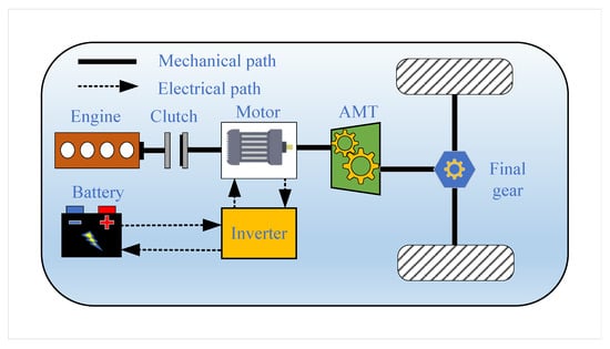
Figure 1.
The structure of the hybrid powertrain.

Table 1.
The parameters of the vehicle.
2.1. Vehicle Dynamics Model
The focus of this paper is on the exploration of energy management strategy and the performance of hybrid systems, including dynamics and economy. It does not need to deal with the lateral forces and vertical motions that the vehicle is subjected to during the driving process. Therefore, only the longitudinal dynamics model is modeled. Since the engine and motor are coaxially connected, the relationship between the resulting driving torque and the power coupling torque can be expressed as follows:
where is the wheel driving torque, and is the engine torque and motor torque, respectively, is the AMT ratio, is the final gear ratio, is the transmission efficiency, and is the braking torque. According to the power balance formula, the driving torque required by the wheels during the driving process of the vehicle can be shown as follows:
where m represents the vehicle mass, g stands for the gravity acceleration, f denotes the rolling resistance coefficient, is the road angle, means the air resistance coefficient, A is the frontal area, indicates the air density, v is the vehicle velocity, is the rotating mass coefficient, and is the wheel radius.
2.2. Power Source Model
The engine burns fuel in the cylinder to produce a high temperature and pressure gas that drives the piston in an up-and-down reciprocating motion. The entire process is complex and involves several disciplines, and it is difficult to express its nonlinear characteristics by mathematical models. Therefore, the engine model is simplified by using a data modeling method based on engine data. The fuel consumption of the engine can be expressed as follows:
where is engine fuel consumption, and means fuel density. is the fuel consumption rate. is the fuel consumption per unit time. The fuel consumption rate can be obtained by fitting a function to the data collected by the engine, which can be expressed as follows.
The fuel consumption rate is obtained as a function of the current engine speed and torque, and engine fuel consumption rate data are shown in Figure 2a.
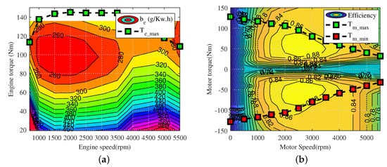
Figure 2.
The map of the engine for (a) and efficiency map of the motor for (b).
In this paper, a permanent magnet synchronous motor is adopted as another power source, which has a simple structure, reliable operation, easy maintenance, high output torque, and high power density. It can be used either as a drive motor or as a generator. The two operating modes of drive and power generation can be indicated as follows:
where is the motor power, is the motor speed, and is the motor efficiency; it can be obtained according to the motor efficiency in Figure 2b. When the motor is driving, the motor torque is positive, and when the motor is generating, the motor torque is negative.
2.3. Battery Model
An internal resistance open-circuit model based on the battery terminal voltage and internal resistance characteristics [30] was developed without considering the effect of power variation on battery charging and discharging performance. The equivalent circuit is shown in Figure 3a. According to Kirchhoff’s voltage law, the equation for calculating the load current is derived for modeling. Based on the equivalent circuit, the battery pack voltage U is obtained as follows:
where is the battery open-circuit voltage, is the battery current, is the battery internal resistance, and means the battery output power. According to the Equation (6), the battery current can be expressed as follows.
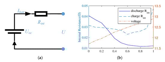
Figure 3.
model for (a) and Internal resistance and open-circuit voltage for (b).
Battery SOC is used to calculate the sum of charge and discharge. Battery SOC is calculated as the sum of the charging and discharging currents, which results in a change in battery charge.The specific expression can be expressed as follows:
where is the capacity of the battery. Neglecting the effects of battery temperature and battery life on the internal resistance of the battery, the variation of internal resistance with SOC is shown in Figure 3b. According to the Equations (7) and (8), the rate of change of SOC is shown as follows.
3. Driving Pattern Recognition Based on FFELM
3.1. Selection of Typical Driving Cycles
Due to the limitations of the existing experimental conditions and the complexity of the actual vehicle driving condition data, this paper combines the existing European standard driving cycles as analysis samples. According to different traffic conditions and vehicle driving areas, the standard driving cycles can be divided into three categories: urban, suburban, and high-speed. Urban congested road condition refers to the vehicle driving in the center of the city: The traffic flow is large, and road approach congestion leads to frequent vehicle starts and low speed; thus, NYCC and NewYorkBus are selected as the reference driving cycles. The suburban driving cycle means that the vehicle often drives at medium speed with fewer traffic lights; thus, the vehicle stops less often and for a shorter period of time. Therefore, ECE_EUDC_LOW and UDDS are selected as the reference driving cycles. The highway driving cycle refers to the vehicle driving speed being higher than the normal highway, and most of the time, it is at high speed, and the number of stops is lower. Therefore, HWFET and US06 are selected as the reference conditions. The speed curves of each reference driving cycle are shown in Figure 4.
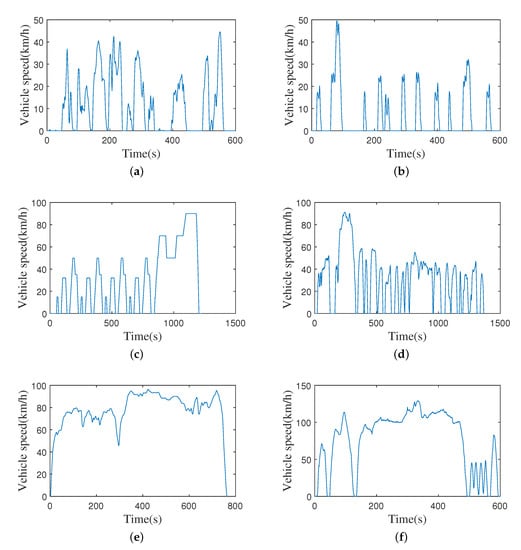
Figure 4.
(a) NYYC. (b) NewYork bus. (c) ECE_EUDC_LOW. (d) UDDS. (e) HWFET. (f) US06.
In order to improve the accuracy and real-time performance of driving cycle classification, this paper selects 11 important driving condition feature parameters for analysis according to the literature [24,25], including average speed , maximum speed , maximum acceleration , average value of the acceleration , the maximum deceleration , the average value of the deceleration , idle time ratio , acceleration time ratio , deceleration time ratio , constant speed time ratio , and idle times in the entire driving cycle. The specific data are shown in Table 2. From Table 2, It can be seen that the amount of sample data for each driving cycle is too small, and achieveing high training and recognition accuracy is difficult. Therefore, the method shown in Figure 5 is used to segment the driving cycles and to calculate the feature parameters of each driving cycle block to increase sample data. In this paper, each typical driving cycle is equally divided by the 120 s period using the above method.
Table 2.
The main characteristic parameters of three typical driving conditions.
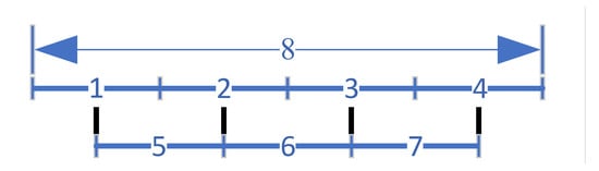
Figure 5.
The method of segment for driving conditions.
In order to further analyze the influence of feature parameters, Principal Component Analysis (PCA) was performed on the collected data. Calculation results of the principal component matrix are shown in Table 3. Select the largest two components to form the component matrix shown in Table 4. It can be seen from Table 4 that component 1 has a great influence on the first seven feature parameters, and component 2 has a great influence on the last four feature parameters. Therefore, the importance of the input feature parameters is listed in the order listed in Table 4.
Table 3.
The contribution rate of the principal component.
Table 4.
The component matrixl component.
3.2. Basic Extreme Learning Machine
The extreme learning machine (ELM) [31] is a Single-Layer Feedforward Neuron Network (SLFN) that is originally proposed by Guang-Bin Huang, Qin-Yu Zhu, and Chee-Kheong Siew at Nanyang Technological University in 2004 and presented at the IEEE International Joint Conference, and it intends to improve the Backward Propagation (BP) algorithm to improve learning efficiency and to simplify the setting of learning parameters. The standard single hidden layer neural network structure is shown in Figure 6. Specifically, SLFN consists of an input layer, a hidden layer, and an output layer.
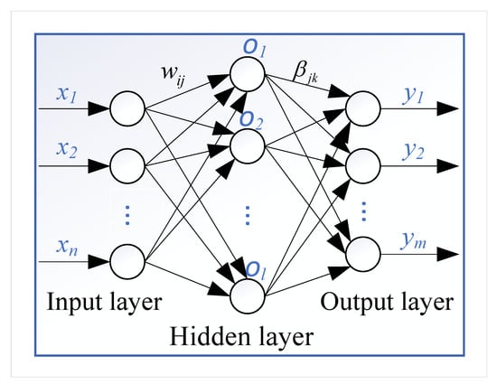
Figure 6.
The structure of ELM.
ELM is a new fast learning algorithm for SLFN, and ELM can randomly initialize the input weights and bias and obtain the corresponding output weights. Suppose the input layer has N random samples , which are the input sample data and corresponding output sample data . A single hidden layer neural network with L hidden layer nodes can be expressed as follows:
where is the activation function, is the Input weight, is the output weight, and is the bias of the i-th neuron. The objective of single hidden layer neural network learning is to minimize the error in the output, which can be expressed as follows.
There exist , , and such that the following is the case.
The above formula simplifies into the following:
with
In order to train a single hidden-layer neural network, ,, and are used.
Since the ELM training network input weights and hidden layer bias are random values and H is fixed at this point, only the output weights need to be solved. Therefore, the output weights can be obtained by the following equation:
where is the Moore–Penrose generalized inverse of H.
3.3. Feature Fusion Extreme Learning Machine FFELM)
Although ELM has a simple structure, fast learning speed, and good generalization, it may cause poor stability due to the random assignment of input weights and hidden layer bias [32,33]. In addition, there may be interactions between the features in the sample data. Therefore, an extreme learning machine that effectively fuses the features is used to improve the stability and accuracy of the classification problem [34]. A block diagram of the extreme learner network for Feature Fusion Extreme Learning Machine (FFELM) is shown in Figure 7. The entire network is divided into three parts: the kernel mapping, the coefficient weighting, and the classification layer. The first and second of these parts implement data feature fusion. The layers of this network are connected with weight matrices , , , and . The individual weight matrices are calculated for training purposes.
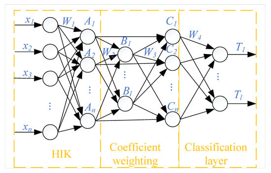
Figure 7.
The structure of FFELM.
The specific formulation is as follows: first input feature data , which corresponds to the output label features . To avoid random assignments of input weight , the Histogram Intersection Kernel (HIK) function is used to map input data X to ; thus, we have the following:
where includes the Mapping Functions. ELM is then used to train weight :
where is the Moore–Penrose generalized inverse of A:
with B as the input of ELM-AE [33], and w and bias are randomly assigned activation function ; at this time, the hidden layer output features , with B as the output of ELM-AE.
Finally, ELM is used again to output the weight , and training is completed.
4. EMS Based on Driving Condition Identification
According to previous studies, the initial values of battery SOC before driving, the type of driving conditions, and the driving distance have a great influence on the real-time energy management strategy of the vehicle. Therefore, this paper proposes a real-time energy management strategy that integrates three factors to improve fuel economy. As shown in Figure 8, the proposed strategy is divided into three parts: (1) offline optimization strategy, (2) online optimization strategy, and (3) real-time driving condition identification.
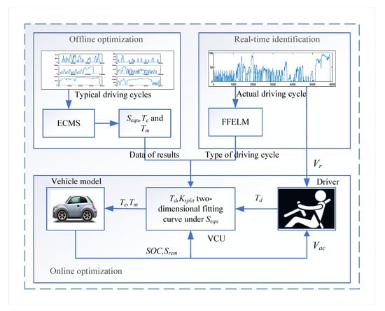
Figure 8.
The structure of the proposed strategy.
According to what is discussed in Section 3.1, driving conditions are classified into six categories based on the characteristic parameters of each condition, and FFELM is used for training classification recognition. In addition, the initial values of battery SOC and driving distance are very important for vehicle energy strategies; therefore, in order to combine these two, the equivalent distance parameter is introduced according to the literature [14]. Considering that there is a relationship between the remaining power and the remaining distance, the expression is as follows:
where is the remaining distance, is the maximum distance in pure electric mode, indicates the remaining charge, is the instantaneous value of the battery charge during vehicle driving, and is the range of the available SOC. and are the upper and lower battery limits, respectively. indicates that the battery can complete the remaining distance in pure electric mode. When , the battery has insufficient power left to complete the rest of the distance in pure electric mode, and the engine is required.
4.1. Offline EMS Optimization
In order to adapt the control strategy to different driving conditions, ECMS is applied offline to optimize the optimal allocation for each typical driving condition in preparation for the application of the online strategy.
4.1.1. Objective Function
According to the actual driver demand power of the vehicle, the actual output power of the engine and motor is reasonably allocated within the power range of the engine and motor such that the sum of the equivalent fuel consumption of the instantaneous fuel consumption of the engine and the power consumption of the motor is minimized [35]; thus, the objective function can be shown as follows:
where is J the total consumption, and denote the initial time and final time, respectively, x and u are the system state and control variables respectively, is the instantaneous fuel consumption of the engine, and is the instantaneous equivalent fuel consumption after power conversion. In order to calculate equivalent fuel consumption more accurately, the equivalent charging factor and equivalent discharging factor are introduced, and the equivalent fuel consumption of battery power can be expressed as follows:
where is the fuel mass calorific value.
Since battery SOC’s balance is not well maintained by ECMS alone, a penalty function is introduced to correct the equivalent fuel consumption to maintain it close to the objective SOC [14]. The basic value of the penalty coefficient is taken as 1. When battery SOC is close to the target SOC, the equivalent fuel consumption of the motor power is basically not corrected so that the strategy can reasonably power the engine and motor according to the lowest equivalent fuel consumption. When the battery SOC is higher than the target SOC value, the penalty coefficient is less than 1, and the equivalent fuel consumption of motor power consumption is reduced by the penalty coefficient so that the control strategy is more inclined to use electric power. When battery SOC is lower than the target SOC value, the penalty coefficient is greater than 1, and the equivalent fuel consumption of motor power consumption is increased by the penalty coefficient such that the control strategy is more inclined to use fuel. Moreover, the penalty coefficient in the target SOC near the value of the change should be relatively gentle so that the penalty coefficient on the power distribution can reduce impact; battery SOC deviates from the target SOC, and the speed of change of the penalty coefficient should be intensified by speeding up the response as soon as possible to maintain power balance. In order to make better and effective use of SOC, the penalty function is introduced:
where is the empirical coefficient; here, 0.2 is chosen; is the objective value of SOC, is the minimum value of SOC, and is the SOC at time t; as shown in the figure, when the penalty factor decreases with the increase in SOC, the modified equivalence factor is as follows.
The corrected power equivalent fuel consumption is as follows.
4.1.2. Control and State Variables
Since this paper is aimed at a single-axis parallel structure where the engine and motor are located on the same shaft and the engine speed and motor speed are the same, the distribution of driver demand power can be translated into an equation for the distribution of engine and motor torque. In order to better achieve torque distribution, the power distribution factor is expressed as the formula of the ratio of engine torque to demand torque, and is introduced. When , the engine and the motor drive together, and when , the engine drives and it drives motor to charge the battery. When , the engine torque is the same as the demand torque and the vehicle is in the engine drive-alone mode. When , the engine is not involved in vehicle driving:
where is the demanded power, and are the engine power and motor power, respectively, is the demanded torque, and the demanded speed. Therefore, it can be further expressed as follows.
Optimal control variables are stated as follows.
Changes in state variables with battery power SOC are defined as follows.
The optimization of different initial values of SOC under different driving conditions is conducted by ECMS. As shown in Figure 9a, the optimized data including the power distribution factor, the rate of change of battery SOC, and the driving distance are sorted. The variation of battery SOC and driving distance under a driving condition can be used to obtain the optimal power distribution factor under this condition.
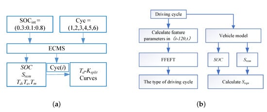
Figure 9.
Offline optimization flow diagram for (a) and real-time recognition flow diagram for (b).
4.2. Real-Time Driving Condition Recognition and Calculation
Based on the current driving conditions, FFELM is used to identify the conditions and to calculate the equivalent distance parameters based on the current battery’s SOC and the distance to the destination. As shown in Figure 9b, the parameters of the operating conditions characterized by 120 periods are calculated, including maximum speed, maximum acceleration, maximum deceleration, etc. These parameters are used as the basis. FFELM identifies the current operating conditions. The equivalent distance is calculated based on the Equation (23), and it is then input to the vehicle controller during the vehicle driving process.
4.3. Online Strategy Optimization
Online torque distribution is achieved by identifying the type of driving condition and the equivalent distance parameters according to the required torque under current driving condition. As shown in Figure 10, online torque distribution is achieved.
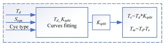
Figure 10.
Online optimization flow diagram.
5. Simulation Results and Discussion
In order to better demonstrate the effectiveness of the proposed strategy, the accuracy of the FFELM identification method is firstly verified. Based on this, the identification method and the proposed strategy are applied to the combined driving condition in real time. The advantages of the proposed strategy are further demonstrated by comparing it with conventional strategy CD-CS.
5.1. Results and Analysis of FFELM
A total of 80 sets of feature data of each typical driving condition block were randomly arranged, with 68 sets of data randomly selected as training data, and ELM and FFELM were used for training. Then, 12 sets of data were randomly selected from 80 sets of data as test data repeatedly. Tests with the trained ELM model and FFELM model and the results are shown in Figure 11. It can be seen from Figure 11a that the accuracy distribution of the test data under ELM is scattered and the accuracy ranges from 0.3 to 1, which is due to the influence of the input weights and biases under random settings. The accuracy of ELM with specific input weights and biases is high for specific test data, but it may be lower or even less than 0.5 for other test data. Therefore, the accuracy under ELM is scattered and unstable. As shown in Figure 11b, the accuracy of the test data under FFELM is mostly greater than 0.7 and is mainly concentrated in the region of 0.8 to 1. The accuracy and stability are better than ELM.
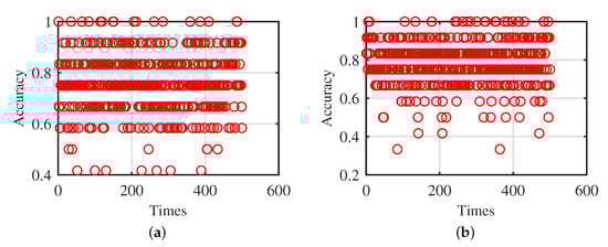
Figure 11.
ELM for (a) and FFELM for (b).
In order to further verify the accuracy and effectiveness of the FFELM recognition algorithm, different algorithms were used to train and test the data of the driving cycles. From the 80 sets of data, 68 sets of data were randomly selected as training data, and 12 sets were used as test data. The LVQ (learning vector quantization), SVM (support vector machine), ELM and FFELM are used for training and testing, respectively. The identification results are shown in Table 5. It can be seen from the results that the LVQ algorithm is not very accurate in testing. On the one hand, in the training process, the weight vector may not converge and the information of each dimension attribute of the input sample may not be fully utilized, which does not reflect the difference in the importance of each dimension attribute in the classification process. Although the accuracy of the SVM algorithm is not very good, stability is good. This is because once the parameters and kernel functions of SVM are determined, accuracy remains relatively stable. Therefore, in order to improve the classification accuracy of SVM, the parameters and kernel functions must be optimized. Moreover, SVM is suitable for sample data with a small amount of data. Although the accuracy of ELM is better than that of SVM, because the weights and thresholds are randomly generated, accuracy is unstable, and the advantage is that the learning speed is fast. FFELM combines kernel mapping and coefficient weighting for the purpose of increasing classification power and robustness. Thus, it shows good accuracy.
Table 5.
Recognition results under different algorithms.
5.2. Results and Analysis of Offline Optimization
In this paper, ECMS is used for the offline optimization of each typical driving condition. Taking the typical driving condition HWFET as an example, the optimization results are shown in Figure 12 with initial values of SOC of 0.8, 0.4 and 0.3, respectively. When the initial value of SOC is 0.8, battery power is sufficient to sustain the entire distance; thus, there is no need to charge the battery during the acceleration process of the entire distance, and the relationship between the demand torque and the power distribution factor at this time is shown in Figure 12a. When the demand torque is less than 20, the power distribution factor is 0, which means that the vehicle runs on pure electric power when the demand torque is less than 20. When the demand torque is greater than 20, the engine and motor jointly drive the vehicle; thus, the ratio of engine torque to demand torque is less than 1 and greater than 0. The red circled points are the optimal power distribution factor corresponding to the optimized demand torque, and the blue line is the fitted curve. When the initial value of SOC is 0.4, the power is not enough to sustain the entire distance; thus, the entire driving distance needs both battery discharge and battery charge. When battery SOC is less than the battery target value, the battery is charged. Therefore, as shown in the figure, the distribution rate is both less than 1 and greater than 1. When the distribution rate is greater than 1, the vehicle is driven by the engine and the battery is charged at the same time. The red circled points are the optimal power distribution factor under the optimization results, and the blue line is the fitted curve. When the initial value of SOC is 0.3, it cannot run purely on electricity at all; thus, the entire driving process needs to be driven by the engine and the battery needs to be charged at the right time. Therefore, the distribution ratio is always greater than 1. The red circled points are the optimal power distribution factor after optimization, and the blue line is the fitting curve.
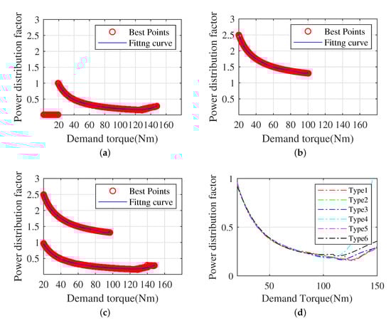
Figure 12.
The results of different SOC. (a) SOC = 0.8; (b) SOC = 0.4; (c) SOC = 0.3; (d) fitting curves under different type of driving cycles.
According to the above description, the best power distribution factor fitting curves for different typical driving cycles can be obtained using the same method. The fitted curves for each driving condition are shown in Figure 12d. Under online optimization, FFELM can identify the type of driving conditions, and the best power distribution factor can be obtained from the fitted curve by using the current SOC, , and demand torque. Thus, the online real-time power distribution can be realized.
5.3. Results and Analysis under Different Strategies
In order to prove the effectiveness of the proposed strategy, the proposed strategy is validated by using a combined driving cycle. The established combined driving cycles are shown in Figure 13a. It consists of six different driving cycles, including urban congestion, urban suburban, and highway conditions. The results of FFEFT identification are shown in Figure 13b. It can be seen that the identification method can effectively identify the type of combined driving conditions.
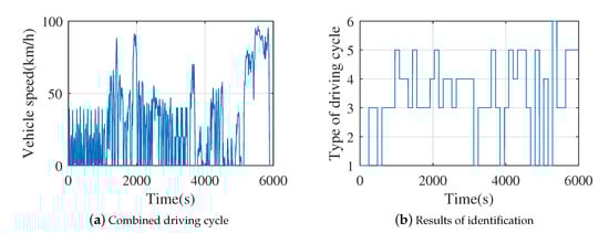
Figure 13.
Combined driving cycle and results of identifications.
Taking the initial value of SOC as 0.6, the optimization results of the three strategies under the combined driving conditions are shown in Table 6. Compared with the CD-CS strategy, the equivalent fuel consumption under ECMS and the proposed strategy is improved by 8.96% and 10.21%, respectively. Figure 14 shows the trajectory of the SOC under the three strategies during vehicle driving. It can be seen from the figure that the decreasing trend of SOC for the three strategies does not differ much in the first 1000 s. This is due to the fact that the vehicle is driving at a speed less than 40 km/h, the demand torque is not large in urban congested driving conditions, and most of it is in pure electric driving. In time 1000 s to 3500 s, the speed increases from low speed to high speed and then turns to medium speed, and the corresponding torque also increases from small torque to large torque by turning to medium torque. Because the CD-CS strategy is in CD mode with priority battery drive, battery SOC decreases the fastest. ECMS and the proposed strategy are the optimal allocation of engine and motor at each moment, but the proposed strategy decreases slower compared to ECMS because the equivalent distance factor is calculated at any time in the proposed strategy to keep the power limit. From 3500 s to 5000 s, the CD-CS strategy is in the CS mode and SOC keeps fluctuating around the SOC objective. The decreasing trend of SOC under ECMS and the proposed strategy is still similar to the previous paragraph. When the time is longer than 5000 s, the vehicle is mostly driven at high speed, and the required torque increases suddenly; thus, the engine and motor need to drive together, and the motor torque increases, and battery SOC decreases faster.
Table 6.
Comparison of equivalent energy consumption when the initial SOC is 0.6.
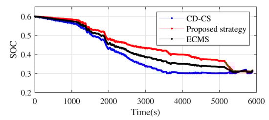
Figure 14.
The results of the SOC under three control strategies.
Figure 15 shows the engine operating points for the optimization results under ECMS and the proposed strategy. The engine operating point under the proposed strategy is closer to the engine’s high efficiency region than the ECMS strategy.
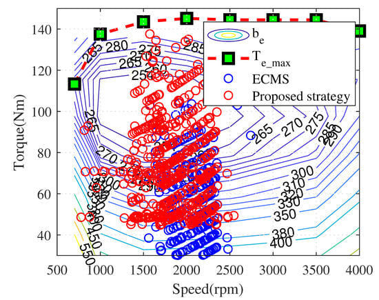
Figure 15.
Engine operation points of ECMS and proposed strategy.
Figure 16 shows the relationship between engine torque and demand torque for different strategies. Since the single-shaft parallel hybrid system is studied in this paper, the required torque of the drive is provided by the engine torque and the electric motor. It reflects the working state of the engine at each time point. In Figure 16a, it can be seen that, under the CD-CS strategy, the engine is not involved in driving during the CD mode, except when the demand torque is high, and the engine is not involved in driving in the other parts, which mainly involves the electric drive. After entering the CS mode, the engine is involved in driving and charging the battery. Comparing Figure 16b with Figure 16c, the engine torque changes similarly to ECMS in the first 2000 s time range. However, as the distance traveled increases, the proposed strategy will plan the torque distribution according to the type of driving conditions and the remaining distance driven.
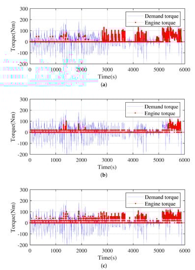
Figure 16.
The results of different strategies. (a) The engine torque of CD-CS; (b) the engine torque of ECMS; (c) the engine torque of the proposed strategy.
6. Conclusions
In this paper, a real-time energy management strategy based on driving condition recognition is proposed. First, an FFELM identification method with high stability and accuracy is used to train six typical driving conditions, which provides the basis for identification under combined driving conditions. Second, the six typical driving conditions are optimized offline using ECMS. By collating the data of optimization results under each driving condition, the optimization results were analyzed based on the equivalent distance coefficients of battery SOC and driving distance. The optimal power distribution factor for each condition optimization is also provided by fitting the data to help the real-time management strategy. Finally, to demonstrate the effectiveness of the proposed strategy, the real-time energy management strategy under mixed driving conditions is used and compared with CD-CS strategy and ECMS strategies.
The comparison between ELM and FFELM for raw data identification shows that FFELM is more accurate and stable than ELM. In the simulation experiments for verifying the effectiveness of the proposed strategy, it is shown that the proposed strategy improves fuel economy by 10.21% and the computation time is slightly longer than that of CD-CS. This means that the proposed strategy has a great potential to save fuel compared to the rule-based strategy and is also effective in real-time control. The equivalent fuel consumption of the proposed strategy is 7.12 L/km compared to the equivalent fuel consumption of ECMS of 7.31 L/km, which is a 2.5% improvement. This shows that the proposed strategy can be adjusted in real-time to achieve optimal fuel economy. Therefore, the proposed strategy has great advantages in fuel economy in real-time and practicality for different driving conditions.
Although the proposed strategy has greatly improved real-time fuel economy and the application of complicated driving conditions, the extraction of typical driving cycle data in this paper are all from the European standard driving cycles and the selection of the features of the road condition data has a great influence on the recognition accuracy of the driving conditions. Therefore, in future work, we will collect the driving condition data that meet the actual driving characteristics of Chinese roads and establish the driving condition recognition model on this basis to improve recognition accuracy.
Author Contributions
H.Z. managed the conceptualized project. P.Q. designed the energy management strategy, completed the modeling and simulation, and wrote the manuscript. P.W. and T.P. collected the data. P.Q. and H.Z. contributed to the validation and analysis of the results and reviewed the writing. All authors have read and agreed to the published version of manuscript.
Funding
Supported by National Natural Science Foundation of China (61573304).
Conflicts of Interest
The authors declare no conflict of interest.
References
- Sabri, M.F.M.; Danapalasingam, K.A.; Rahmat, M.F. A review on hybrid electric vehicles architecture and energy management strategies. Renew. Sustain. Energy Rev. 2016, 53, 1433–1442. [Google Scholar] [CrossRef]
- Liu, Y.; Gao, J.; Qin, D.; Zhang, Y.; Lei, Z. Rule-corrected energy management strategy for hybrid electric vehicles based on operation-mode prediction. J. Clean. Prod. 2018, 188, 796–806. [Google Scholar] [CrossRef]
- Chen, Z.; Liu, Y.; Ye, M.; Zhang, Y.; Li, G. A survey on key techniques and development perspectives of equivalent consumption minimisation strategy for hybrid electric vehicles. Renew. Sustain. Energy Rev. 2021, 151, 111607. [Google Scholar] [CrossRef]
- Shi, D.; Liu, S.; Cai, Y.; Wang, S.; Li, H.; Chen, L. Pontryagin’s minimum principle based fuzzy adaptive energy man-agement for hybrid electric vehicle using real-time traffic information. Appl. Energy 2021, 286, 116467. [Google Scholar] [CrossRef]
- Liu, Y.; Li, J.; Chen, Z.; Qin, D.; Zhang, Y. Research on a multi-objective hierarchical prediction energy management strategy for range extended fuel cell vehicles. J. Power Sources 2019, 429, 55–66. [Google Scholar] [CrossRef]
- He, X.; Wu, X. Eco-driving advisory strategies for a platoon of mixed gasoline and electric vehicles in a connected vehicle system. Transp. Res. Part Transp. Environ. 2018, 63, 907–922. [Google Scholar] [CrossRef]
- Peng, J.; He, H.; Xiong, R. Rule based energy management strategy for a series–parallel plug-in hybrid electric bus optimized by dynamic programming. Appl. Energy 2017, 185, 1633–1643. [Google Scholar] [CrossRef]
- Overington, S.; Rajakaruna, S. High-efficiency control of internal combustion engines in blended charge depletion/charge sustenance strategies for plug-in hybrid electric vehicles. IEEE-Trans-Actions Veh. Technol. 2014, 64, 48–61. [Google Scholar] [CrossRef]
- Son, H.; Kim, H.; Hwang, S.; Kim, H. Development of an advanced rule-based control strategy for a PHEV using machine learning. Energies 2018, 11, 89. [Google Scholar] [CrossRef] [Green Version]
- Chen, Z.; Gu, H.; Shen, S.; Shen, J. Energy management strategy for power-split plug-in hybrid electric vehicle based on MPC and double Q-learning. Energy 2022, 245, 123182. [Google Scholar] [CrossRef]
- Garcia, A.; Carlucci, P.; Monsalve-Serrano, J.; Valletta, A.; Martínez-Boggio, S. Energy management strategies comparison for a parallel full hybrid electric vehicle using Reactivity Controlled Compression Ignition combus-tion. Appl. Energy 2020, 272, 115191. [Google Scholar] [CrossRef]
- Wu, Y.; Ravey, A.; Chrenko, D.; Miraoui, A. Demand side energy management of EV charging stations by approximate dynamic programming. Energy Convers. Manag. 2019, 196, 878–890. [Google Scholar] [CrossRef] [Green Version]
- Liu, J.; Chen, Y.; Li, W.; Shang, F.; Zhan, J. Hybrid-Trip-Model-Based Energy Management of a PHEV With Computation-Optimized Dynamic Programming. IEEE Trans. Veh. Technol. 2018, 67, 338–353. [Google Scholar] [CrossRef]
- Xie, S.; Hu, X.; Xin, Z.; Brighton, J. Pontryagin’s minimum principle based model predictive control of energy management for a plug-in hybrid electric bus. Appl. Energy 2019, 236, 893–905. [Google Scholar] [CrossRef] [Green Version]
- Sánchez, M.; Delprat, S.; Hofman, T. Energy management of hybrid vehicles with state constraints: A penalty and implicit Hamiltonian minimization approach. Appl. Energy 2020, 260, 114149. [Google Scholar] [CrossRef]
- Shangguan, J.; Guo, H.; Yue, M. Robust energy management of plug-in hybrid electric bus con-sidering the uncertainties of driving cycles and vehicle mass. Energy 2020, 203, 117836. [Google Scholar] [CrossRef]
- L.ü, X.; Wu, Y.; Lian, J.; Zhang, Y.; Chen, C.; Wang, P.; Meng, L. Energy management of hybrid electric vehicles: A review of energy optimization of fuel cell hybrid power system based on genetic algorithm. Energy Convers. Manag. 2020, 205, 112474. [Google Scholar] [CrossRef]
- Hemi, H.; Ghouili, J.; Cheriti, A. A real time energy management for electrical vehicle using combination of rule-based and ECMS. IEEE Electr. Power Energy Conf. 2013, 2013, 1–6. [Google Scholar]
- Li, H.; Ravey, A.; N’Diaye, A.; Djerdir, A. Online adaptive equivalent consumption minimization strategy for fuel cell hybrid electric vehicle considering power sources degradation. Energy Convers. Manag. 2019, 192, 133–149. [Google Scholar] [CrossRef]
- Choi, K.; Byun, J.; Lee, S.; Jang, I.G. Adaptive Equivalent Consumption Minimization Strategy (A-ECMS) for the HEVs with a Near-Optimal Equivalent Factor Considering Driving Conditions. IEEE Trans. Veh. Technol. 2021, 71, 2538–2549. [Google Scholar] [CrossRef]
- Gao, J.P.; Zhu, G.M.G.; Strangas, E.G.; Sun, F.C. Equivalent fuel consumption optimal control of a series hybrid electric vehicle. Proc. Inst. Mech. Eng. Part J. Automob. Eng. 2009, 223, 1003–1018. [Google Scholar] [CrossRef]
- Sinoquet, D.; Rousseau, G.; Milhau, Y. Design optimization and optimal control for hybrid ve-hicles. Optim. Eng. 2011, 12, 199–213. [Google Scholar] [CrossRef] [Green Version]
- Marano, V.; Tulpule, P.; Stockar, S.; Onori, S.; Rizzoni, G. Comparative study of different control strategies for plug-in hybrid electric vehicles. In Proceedings of the 9th International Conference on Engines and Vehicles, Naples, Italy, 13 September 2009. [Google Scholar]
- He, H.; Sun, C.; Zhang, X. A method for identification of driving patterns in hybrid electric vehicles based on a LVQ neural network. Appl. Energy 2012, 5, 3363–3380. [Google Scholar] [CrossRef]
- Song, K.; Li, F.; Hu, X.; He, L.; Niu, W.; Lu, S.; Zhang, T. Multi-mode energy management strategy for fuel cell electric vehicles based on driving pattern identification using learning vector quantization neural network algorithm. J. Power Sources 2018, 389, 230–239. [Google Scholar] [CrossRef]
- Chen, Z.; Li, L.; Yan, B.; Yang, C.; Martínez, C.M.; Cao, D. Multimode energy management for plug-in hybrid electric buses based on driving cycles prediction. IEEE Trans. Intell. Transp. Syst. 2016, 17, 2811–2821. [Google Scholar] [CrossRef]
- Denis, N.; Dubois, M.R.; Dubé, R.; Desrochers, A. Blended power management strategy using pattern recognition for a plug-in hybrid electric vehicle. Int. J. Intell.-Transp. Syst. Res. 2016, 14, 101–114. [Google Scholar] [CrossRef]
- Wei, C.; Chen, Y.; Li, X.; Lin, X. Integrating intelligent driving pattern recognition with adaptive energy management strategy for extender range electric logistics vehicle. Energy 2022, 247, 123478. [Google Scholar] [CrossRef]
- Qiang, P.; Wu, P.; Pan, T.; Zang, H. Real-Time Approximate Equivalent Consumption Minimization Strategy Based on the Single-Shaft Parallel Hybrid Powertrain. Energies 2021, 14, 7919. [Google Scholar] [CrossRef]
- Tian, X.; He, R.; Sun, X.; Cai, Y.; Xu, Y. An ANFIS-based ECMS for energy optimization of parallel hybrid electric bus. IEEE Trans. Veh. Technol. 2019, 69, 1473–1483. [Google Scholar] [CrossRef]
- Huang, G.B.; Zhu, Q.Y.; Siew, C.K. Extreme learning machine: Theory and applications. Neurocomputing 2006, 70, 489–501. [Google Scholar] [CrossRef]
- Huang, G.B.; Zhou, H.; Ding, X.; Zhang, R. Extreme learning machine for regression and multiclass classification. IEEE Trans. Syst. Man, Cybern. Part (Cybern.) 2011, 42, 513–529. [Google Scholar] [CrossRef] [PubMed] [Green Version]
- Kasun, L.L.C.; Zhou, H.; Huang, G.B.; Vong, C.M. Representational learning with ELMs for big data. IEEE Intell. Syst. 2013, 28, 31–34. [Google Scholar]
- Aziz, S.; Youssef, F. Traffic sign recognition based on multi-feature fusion and ELM classifier. Procedia Comput. Sci. 2018, 127, 146–153. [Google Scholar] [CrossRef]
- Chen, S.Y.; Wu, C.H.; Hung, Y.H.; Chung, C.T. Optimal strategies of energy management integrated with transmission control for a hybrid electric vehicle using dynamic particle swarm optimization. Energy 2018, 160, 154–170. [Google Scholar] [CrossRef]
Publisher’s Note: MDPI stays neutral with regard to jurisdictional claims in published maps and institutional affiliations. |
© 2022 by the authors. Licensee MDPI, Basel, Switzerland. This article is an open access article distributed under the terms and conditions of the Creative Commons Attribution (CC BY) license (https://creativecommons.org/licenses/by/4.0/).