Energy Consumption Forecasting for the Digital-Twin Model of the Building

Abstract

The aim of the paper is to propose a new approach to forecast the energy consumption for the next day using the unique data obtained from a digital twin model of a building. In the research, we tested which of the chosen forecasting methods and which set of input data gave the best results. We tested naive methods, linear regression, LSTM and the Prophet method. We found that the Prophet model using information about the total energy consumption and real data about the energy consumption of the top 10 energy-consuming devices gave the best forecast of energy consumption for the following day. In this paper, we also presented a methodology of using decision trees and a unique set of conditional attributes to understand the errors made by the forecast model. This methodology was also proposed to reduce the number of monitored devices. The research that is described in this article was carried out in the context of a project that deals with the development of a digital twin model of a building.

1. Introduction

The electric energy consumption profile in residential buildings in Poland has changed more in recent years than during the previous several decades [1]. During the last two years, the biggest changes were related to the epidemic period and the transition to remote work that have taken place [2]. The electrification of heating in buildings (e.g., heat pumps, air conditioning) has a significant impact on changing the shape of the electricity demand profile [3]. Social behaviour (remote work, longer working day) also affects the daily demand for electric energy [4]. Forecasting the demand for electricity is carried out at the level of the power system [5], by the transmission system operator (TSO) and DSM/DSR service aggregators, by energy sellers and distributors (to plan the sales volume), in local government units [6] and in large industry (to plan the purchase volume) [7]. For individual customers (residential buildings), the forecast of annual energy consumption is sufficient in order to select the appropriate tariff. So far, forecasting the daily electric energy demand has not been needed.

The increase in the installed capacity of micro photovoltaic sources in buildings changes methods of settlement for the energy fed into the grid from these sources. This change is most often less beneficial for prosumers, e.g., selling energy at the market price. In Poland, the sale of surplus energy from micro photovoltaic sources begins in 2022 [8]. Therefore, it will be most cost-effective to use the energy directly in the building or store it in batteries. Consequently, there is a need for daily energy consumption forecasting in buildings. Forecasting the daily demand for electricity may also be used for energy consumption reduction methods and planning the use of energy storage. In addition, it is possible to estimate the energy consumption of devices that have the largest share in energy consumption and indicate it to the user. This information is of great importance in planning the daily energy consumption by individual devices (based on intelligent recommendation system) in the context of balancing energy with a photovoltaic. Predicting the energy usage in order to use it directly in the building, along with solutions empowering the smaller prosumers in the context of selling their products, e.g., as presented in [9], can give the prosumers the most out of their product, and it can encourage others to install micro photovoltaic sources.

1.1. Research Background

The research presented in this article was carried out as part of a larger scientific project. The project’s main task was to develop a model of the building in the digital twin convention [10]. As part of the conducted project, we installed an electric energy consumption monitoring system for the entire building and for almost all electrical devices in the selected buildings. The schema of the digital-twin model is presented in Figure 1. The energy usage data from different devices were monitored and stored in the databases.

The most important feature of the digital-twin model is the ability to analyse data on an ongoing basis and update daily electricity consumption based on the data. This is particularly important in the case of a model aimed at reducing electricity consumption, matching a photovoltaic source to energy demand or the use of electricity storage. In such cases, the model can be used to control the operation of devices in the building (e.g., by making suggestions to the user). Because of this, one of the most important modules of the digital-twin model is the electric energy demand prediction. This is a particularly important element because in modern buildings, according to currently enforced energy consumption standards, the most advantageous energy medium is electricity, used both to power household appliances and heating. Using the measured energy consumption (current and archival), we conducted prediction studies of electricity demand in the building for the next 24 h.

The developed solution is dedicated to individual customers—households and small service facilities. As a result, it was necessary to develop a cheap system—the cost of installation and operation of which would not exceed the possible economic effect. In this case, the cost is mainly related to the purchase of measurement and control infrastructure. Therefore, the proposed solution functions on a limited amount of data—from electricity meters, weather forecasts and the calendar. It is also worth noting that measuring energy consumption for almost every device in a residential building is pointless, because we estimate that approx. 20% of the devices in a building consume approx. 80% of electricity. These are usually the same devices, regardless of the building (e.g., heat pump, electric cooker, washing machine, refrigerator, etc.). Therefore, the measurement should be carried out only for the most energy-intensive devices. The second issue is energy consumption by measuring systems. Each measuring point consumes approx. 0.5–1 W, which for 100 devices increases the annual energy consumption to about 400 kWh.

1.2. Aim of the Paper

The article focuses on the module of the digital-twin model, which is responsible for the electric energy demand prediction. The aim of the paper is to propose our approach for forecasting energy consumption in residential buildings for the next 24 h and investigate the usefulness of monitoring the energy consumption of selected household appliances in order to improve the quality of forecasts.

This problem of forecasting the energy demand has been analysed in the literature before, but our project has some unique properties, the analysis of which may be useful in broadening our knowledge on a given topic. Before describing our research, we will present the current state of knowledge.

1.3. Related Work

Energy usage can be represented as a time series. The classical method for forecasting this type of data is an ARIMA model. The paper [11] presents the literature survey of using ARIMA models for the problem of forecasting energy demand. ARIMA was also used for the problem in papers [12,13]. The paper [14] presents more advanced methods: regression analysis, decision trees and neural networks. The authors prove that the decision tree and neural network models may be viable alternatives to the stepwise regression model. Linear regression and multiple linear regression models were used by many authors for forecasting energy consumption, e.g., in [15,16,17].

In [18], the authors present a regression and statistical technique for predicting the energy usage, which could be used for different types of buildings. Their forecasting model works only on one dependent variable—daily electricity consumption—and a few explanatory variables, focused mostly on the weather conditions. This model does not take into account the energy consumption of the devices.

A very popular model for forecasting energy demand is the long-short term memory (LSTM) deep learning model. Two different architectures of LSTM were tested in [19]. The authors showed that standard LSTM performed well in one-hour resolution data. The paper [20] proposed using LSTM to predict energy demand. What is interesting, the authors also present the explanation of the model based on the attributes from the t-SNE. The disadvantage may be the fact that t-SNE may produce some non-interpretable features, which can lead to difficulty in understanding the model. The LSTM method was also used in [21], together with random forest (RF) and convolutional neural networks (CNNs). In the literature, we can find a lot of combinations of the LSTM approach with other neural network models, which are used for electric load forecasing. In [22], the authors propose a hybrid CNN-LSTM model for short-term forecasting. In their approach, the CNN layer is responsible for feature extraction, where LSTM is responsible for sequence learning. Another hybrid model—Multi-Sequence LSTM with recurrent neural network (RNN)—was proposed in [23]. The hybrid approach was also presented in [24] where LSTM was combined with the stationary wavelet transform (SWT) technique.

A different neural network—Elman neural network—with K-medoids algorithm was proposed in [25] as a forecasting prosumer model. The authors of [26] propose using a deep learning model based on the multi-headed attention with the convolutional recurrent neural network for forecasting the residential energy consumption. The proposed solution takes into account not only the whole energy consumption time series, but also data about the usage of groups of devices. The experiments were based on the dataset that included an additional three sub-meters—for devices in the kitchen, in the laundry room and the last corresponding to an electric water-heater and air-conditioner. However, the used dataset did not contain information about the energy usage of each appliance separately, but only about the total energy consumption for each of the three groups. Furthermore, it is important to highlight that the used dataset of the UCI household electric power consumption concerned the measurements gathered between December 2006 and November 2010. Since then, energy consumption characteristics may have changed significantly, especially after the COVID-19 pandemic, which caused us to change our habits (remote work, longer working day). For this reason, these data may already have become outdated.

Another approach to the specific problem is presented in [27]. The authors did not use Machine Learning or Artificial Intelligence models but, using the experts’ analysis of different factors and socio-demographic factors, they created a statistical model (Bayesian model) to predict the energy consumption. In the paper [28], the authors present their agent-based model to simulate the household electricity usage behaviour in several cold regions. The model includes basic information about the residents, their energy-saving awareness, their usage of appliances and the impact of energy-saving management. This model, however, was created based on a questionnaire survey. The advantage of this approach is the fact that the data were obtained from many people (362 valid questionnaires). It would be difficult to monitor so many buildings using sensors, especially if we would like to monitor all the devices used in the home, but, on the other hand, data from surveys is not as accurate as data obtained from monitoring sensors. It is also important to point out, that the authors created a general model, not one model for each location. In the paper [29], the authors proposed their approach for modelling the electrical energy consumption profile of residential buildings in Iran. The authors developed a bottom-up method. They created different profiles that consider the number of residents. The models also include the usage of the appliances. However, the proposed models do not operate on changing time series data and do not include real energy usage of the devices. The contribution of the paper focuses on creating profiles for different buildings and not a time series forecasting model. From the cited papers that concern modelling the electrical energy consumption profiles, we can see that including information about the energy usage of the appliances is an important factor that should be taken into account. In [30], a review of modelling home energy management systems (HEMS) was presented. The authors indicate that a significant barrier to the deployment of HEMS can be the problem of modelling the energy usage of each device. Because of this, many works in the literature simplified this problem, and the proposed solutions use only groups of devices. This problem can be eliminated by including incoming, up-to-date data about each of the devices.

A review of forecasting in energy storage applications can be found in [31]. The authors indicate that using new AI algorithms can be considered one of the most promising directions in the field. However, the paper highlights the importance of using explainable AI. The paper [32], reviews the time series forecasting techniques for building energy consumption. The nine forecasting techniques based on the machine learning are analysed. The review did not include the Prophet algorithm that was analysed by us, because this algorithm was proposed in the year of publishing the review. The Prophet model was used in [33] for long-term peak load forecasting in powerplants. The paper indicates that the Prophet model outperforms the well-established Holt–Winters model. The Prophet was also proposed for electrical load forecasting for data of the Elia grid in the paper [34]. It was also successfully used for short-term forecasting for the energy production from the renewable energy sources by the authors of [35]. A similar study—forecasting photovoltaic panel output using Prophet—was presented in [36]. As far as we know, in the literature the Prophet algorithm was not used for the problem of forecasting energy demand in the residential buildings.

Several studies describing the problem of energy demand forecasting are focused on predictive forecasting in industry and not in homes or flats. The paper [11] presents a survey of methods used for energy demand predictions in manufacturing industries. The authors present the set of generic forecasting methods, but also some specifically tailored to the problem methods. As it was highlighted in [37], 81% of their reviewed research was focused on the educational buildings or/and commercial buildings. Only 19% of them were focused on residential buildings. This shows that when it comes to predicting energy consumption in residential homes, our knowledge is still limited, and the focus should be on this research. Additionally, this same paper indicates that the energy consumption predictions for residential building are needed because they represent 21% of the total energy consumption in the US, which is greater than the share of commercial and industrial buildings.

1.4. Contribution

The summary of the main contribution is as follows.

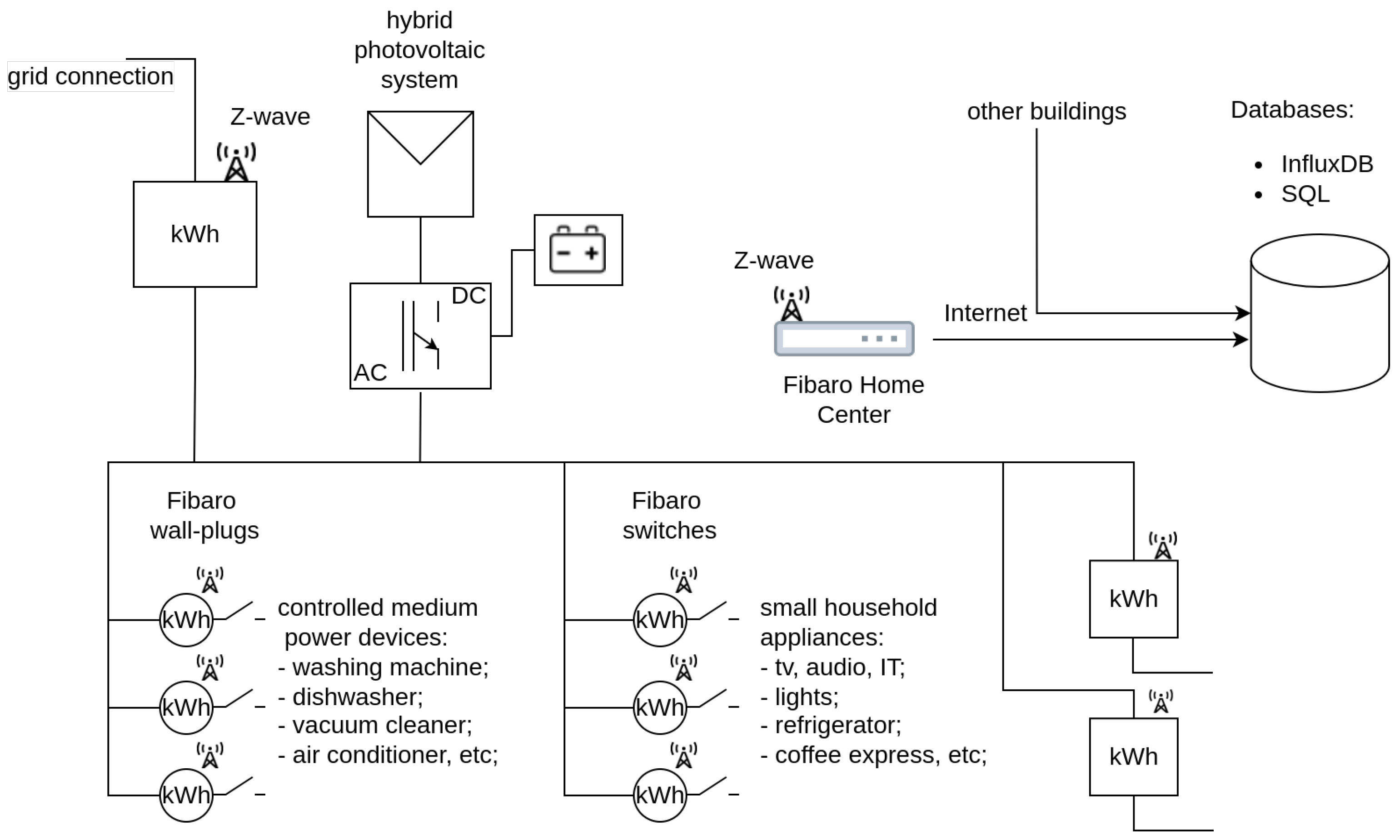
• We propose an approach for forecasting the energy consumption for the next day that is based on data obtained from the digital-twin model of a building. Thanks to this, we can use data describing the energy consumption of the devices used in the building together with data describing the whole energy consumption of the location and the weather data. As far as we know, this approach is unique in comparison with other work.
• In our approach, we focus mostly on residential buildings. In the paper [37], it was highlighted that this direction of research is very important because of the high energy consumption share of this sector. The paper also points out that accurate energy demand predictions in residential houses could be highly beneficial if the forecasts were used to implement successful energy reducing strategies.
• In the research, we used different forecasting methods: naive and linear regression, highly-used LSTM networks (used in [20,21]), but also the Prophet method [38] that, to the best of our knowledge, was not described in the literature in the context of forecasting energy demand in the buildings.
• The proposed models give satisfactory results, and for three models from four locations, we obtained the expected effectiveness of the forecasts (the goal was to obtain less than 25% error).
• In the paper, we also propose our methodology for explaining the model in the interpretable way. As it was mentioned in [37], a lot of data-driven prediction models are black-box models, so they provide limited understanding of the situations, when the model makes a mistake. In our research, we address this problem.
• We use our explanatory methodology in order to limit the number of monitored devices.

2. Materials and Methods

In the research, we considered data from seven different locations. In each of them, the most energy-intensive devices were equipped with the energy consumption meters. Furthermore, the energy consumption for the whole location was monitored. The energy information was saved in the database every few seconds. The data were stored in the InfluxDB database and visualised in the Grafana environment.

Due to the errors of information gathering meters, and after choosing only non-commercial buildings, we used data from four different locations in our research. In our experiments we will refer to them as A, B, C and D. The characteristic of the locations is as follow:

• Location A—flat in a block of flats, 3 people (family 2 + 1).
• Location B—flat in a block of flats, 2 adults.
• Location C—modern detached house, approximately 120 m${}^2$ with electric heating, 3 people (family 2 + 1).
• Location D—detached house, approximately 140 m${}^2$, 4 people (family 2 + 2).

The summary of a type of location and characteristic of observed daily energy consumption can be found in

Table 1. Summary of location characteristics. The type of location, minimum, mean, median and maximum values of observed daily energy consumption are presented for each location.

Location	Type	Min. Energy [kWh]	Mean Energy [kWh]	Median Energy [kWh]	Max. Energy [kWh]
A	Flat	2.14	6.64	6.52	13.89
B	Flat	1.34	3.66	3.30	10.44
C	House	3.92	17.19	17.68	29.68
D	House	6.68	14.65	14.63	34.62

. As can be seen, energy consumption is higher for houses than for flats.

All the buildings are located in the Silesian voivodeship. The gathered datasets consider the period from 1 March 2021 to 28 October 2021. However, due to the lack of some measurements, especially these from the first months of gathering data, and due to some errors in data, the further considered period of data was individual for each location.

A digital-twin model was created for the specific locations, so for C and D it was created for the whole building, and for locations A and B only for the specific flats (not the whole building). However, in order to simplify the nomenclature, we will continue to use the term “digital-twin of the building” regardless of whether it was created for the house or for a flat. Moreover, the prediction of energy consumption was completed separately for each location, i.e., for locations C and D the aim was to predict the energy demand for the whole building, and for locations A and B the aim was to predict the energy demand for the flat.

2.1. Data Preparation

In the first step of the data preparation process, we aggregated the energy-consumption data into hourly intervals for each location. We aggregated data using Grafana, and the data about energy consumption was saved in incremental format. Thanks to this, we could impute missing data, because we had the value before the data gap and the incremented value after the data gap. Based on this information, we could retrieve the information about how much energy was used during the missing period. The missing data were imputed using linear interpolation. We also saved the information about which hourly consumptions were imputed and which are the real values from the database.

In Figure 2 we present the decomposed energy consumption time-series for each location. We present the trend and weekly seasonality components of the time-series. We can observe that the characteristic for each location, especially in terms of weekly seasonality, is different for each location.

In the next step, we added the historical data about weather. We used the information about the temperature that was measured in each hour and the percentage value of the overcast. The historical weather data were the same for all locations because all of them were located close to each other.

In our research, we wanted to predict energy consumption for the next day, so the data had to be aggregated into the daily periods. We added up the energy consumption for each day, calculated the percentage of imputed values for each day, and calculated new attributes describing minimal, maximal and mean values of temperature and overcast for each day. We removed from the data on days for which we had less than 24 hourly observations (mostly the first and the last day from the whole dataset).

We used the information about the percentage of the imputed values to decide which data should be used in training and testing the created predictive models. In order to explain this, we make a small reference to the data format used by LSTM (long short-term memory) models.

In our research, we wanted to use LSTM models. These models are learning from historical data. For each data point, a new vector of historical values (inputs) has to be created. We decided that our historical horizon would be equal to two weeks, so the model learns based on the last 14 values. In our research, we made an assumption that the predictions should be made for the next day, and no later than at 6 p.m. should the user get a forecast of their usage for the next day. Because of this, making prediction for a specific day, the real value from the day before the considered day could not be used for training and recalculating the model. This causes the input for the LSTM model to have values from 15 to 2 days before the considered day. The output of the model was an energy consumption for the specific day. For each day from the available data, we created the row with all inputs (14 values) and output (1 value). We used the information about the percentage of the imputed values in order to decide which of these rows could be used by us in our further experiments. All the rows for which the output has the percentage of the imputation higher than 50% were removed from the dataset (because a forecasting model should not learn imputed values, but the real values observed in the location). Then, for each row, we calculated the mean value of percentage imputed values for the inputs. If the mean value was higher than 50%, the rows were also removed. We adopted a limit of 50% because we assumed that if more than 50% of values—based on which the daily energy usage was calculated—were imputed, then we did not have a realistic value for the day. We wanted to reduce the situation where the model learns from too much artificially entered data while also not deleting too much data.

After data cleaning, we had the data points to be used in our experiments. In our research, we used different types of models, but in order to compare results from different approaches, we used the same dataset for each.

For the data describing the total energy consumption in the location and the historical weather data, we added the information about the energy consumption for the top 10 most energy-consuming devices. These top devices were chosen based on the total energy consumption calculated on the whole available dataset. Because of this, some of these devices (e.g., air conditioning) had varied consumption during the months under consideration, and some appliances had similar energy consumption throughout the whole period. The top 10 most energy-consuming devices in each location were:

• In location A—computer, shower light, recess lighting, outdoor lighting, dinner room lighting, washing machine, Wi-Fi socket, socket under desk, bedroom lamp, hood.
• Location B—fridge, socket for RTV, dishwasher, socket no. 1, socket no. 2, microwave, socket no. 3, air conditioner, socket no. 4, socket no. 5.
• Location C—socket for hot water tank, heater in the bathroom, radiator heater, fridge, socket for the desk, dishwasher, induction stove, fridge in the pantry, socket under TV, socket in the office.
• Location D—fridge, TV-Audio, dishwasher, fridge no. 2, dryer, boiler, TV in kitchen, kettle, socket near the desk, alarm power supply.

It is worth noting that the given descriptions are how the individual sockets are described in the database. However, it is not possible to verify whether the household members have plugged in different devices to particular sockets.

In the data, for some locations, there was also visibly interesting behaviours, such as a sudden decrease in energy consumption for several devices at the same time. These situations took place during the summer months (July, August), so we assume that it was caused by the holiday and the departure of the residents of the building.

To sum up, for each location we created a separate dataset. Each of them included about 7 months of data describing total energy consumption in the location for each day. Any missing data were imputed using linear interpolation. To the dataset we added the historical weather data for each day (mean, minimum and maximum value of temperature and overcast during the day). Then, we also added the data about energy consumption of the top 10 energy-consuming devices. We also stored the information about which data points could be used in training and testing created models. These dates were chosen based on the information about the number of imputed values.

2.2. Experiments

In our research, we wanted to check the best available way to predict the total energy consumption for the next day in the residential buildings. Our aim was to obtain the mean error of the predictions lower than 25%. We wanted to specify which algorithm will give the best results and also what set of the attributes will improve forecasts. In our experiments we wanted to check how the quality of the models changes with incoming data so that the models, if possible, were recalculated for every new data point. We also made the assumption that the first models can be calculated if we have at least 14 data points to train the model on. Because we decided to create data points where inputs have the last historical data from 15 days before, for the LSTM model, in order to start training the model we needed at least 29 days of data. The models were created separately for each location.

2.2.1. Baseline and Linear Regression Models

Our baseline was the naive model. It predicted the value observed in this location exactly a week before. Therefore, if the model had to predict a value for the Saturday, it took the energy consumption from the Saturday of the week before and used it as the prediction.

We also created four models that made predictions based on linear regression. The difference between them was on the number of data used to create linear regression. The used data periods were: 30 days, 14 days, 7 days and 4 days. These are the number of days back to the forecast day based on which the linear regression was determined.

2.2.2. LSTM and Prophet

In the research, we considered two more advanced methods: LSTM network and Prophet. They are typical methods used in the task of time series forecasting.

The LSTM network is a state-of-the-art sequential deep learning method. It is capable of working well on linear and non-linear time series [39]. In our experiments, we used the structure proposed by the Telemanom authors [40]. Our network had two LSTM layers: both had 80 units, and after each of them we added the Dropout layer with dropout equal to 0.3. The activation method was linear. When compiling, we used the adam optimizer and mean squared error (MSE) as a loss metric. For fitting the model we used 35 epochs, a batch size of 64 and split the data into train and validation data in the proportion 85% to 15%. The training of the model stopped when, during 10 epochs, the MSE metric was not improving. The LSTM models were implemented using Python and Keras with Tensorflow. For each model created from the deep networks, input values were standardized before training the model. The standardization was based on the training dataset.

Prophet [38] is an open-sourced library created by Facebook in 2017. Its goal is to analyse time series data and forecast its future values. The Prophet models take into account trends, seasonality and holidays. Multiple seasonalities can be included. The Prophet model can be represented as decomposed time series, and they can be described with the following equation:

$$y\left(t\right)=g\left(t\right)+s\left(t\right)+h\left(t\right)+{ϵ}_t$$

(1)

where $g\left(t\right)$ represents trend function, $s\left(t\right)$ represents seasonality (daily, weekly, yearly), $h\left(t\right)$ represents the holiday effect and ${ϵ}_t$ is the error. An in-depth description of the Prophet algorithm can be found in the paper [41].

The important feature is that the library is possible to use without expert knowledge about time series forecasting. The first results can be obtained without setting any parameters. The user can provide only historical data of a time series in an adequate data format, and they will obtain the forecast of future values. Thanks to this feature, it can be very useful for users without a data science background. On the other hand, the Prophet library is highly customizable, so the more experienced users can add much additional information, that can be useful for the model. The library is available in Python and R. In our experiments, we used the R library version.

In order to check the improvement of forecasts when using different sets of the attributes, we have considered the following cases:

• Using information only about the total energy consumption.
• Using information about the total energy consumption and the weather.
• Using information about the total energy consumption and the energy consumption of the top 10 energy-consuming devices.
• Using information about the total energy consumption, the weather and the energy consumption of the top 10 energy-consuming devices.

The additional attributes (weather attributes and the consumption of the top 10 devices) were added as new channels in LSTM models and as additional regressors in Prophet models. In these cases, we were working with multichannel time series and multiple input forecasting problem.

As it was mentioned before, we wanted to check the quality of the models when new data arrives that may have different characteristics from previous data. Because of this, the LSTM models were recalculated every day, if possible. The quality in time of Prophet models was evaluated based on the cross_validation method that is available in this library. Cross validation for Prophet was also performed every day, if possible, and this simulated a situation where, as new data arrives, the Prophet model is retrained.

The Prophet forecasts also have information about a confidence interval of the prediction. We decided that if the confidence interval is too wide (it is bigger than the predicted value), then we assume that the model could not make a proper decision (we consider it as a lack of the forecast).

We carried out the experiment using two programming languages. The experiments for naive method, linear regression models and Prophet models were conducted using the R language, and LSTM models were created using Python language and Keras library.

3. Results

In our experiments, we considered four locations. We will refer to them as A, B, C and D. The goal of the task was to obtain the mean error of the predictions lower than 25%. The results of the MAPE (mean absolute percentage error) metric for each dataset and each model are presented in

Table 2. The MAPE (mean absolute percentage error) of different model predictions made for 4 locations: A, B, C and D. Results that achieve the MAPE < 25% assumption are marked in bold.

Experiment	MAPE A	MAPE B	MAPE C	MAPE D
val_week_before	43.4	47.66	51.58	31.93
lr_30days	33.58	38.93	40.1	29.6
lr_2weeks	40.86	40.85	41.78	29
lr_1week	43.91	52.25	35.71	32.32
lr_4days	47.58	62.01	32.27	35.75
simple_prophet	34.71	40.69	31.32	27.32
weather_prophet	34.51	40.80	38.93	27.23
devices_prophet	19.9	43.90	18.17	11.1
devices_weather_prophet	20.81	44.57	19.34	12.07
simple_telemony	52.02	49.02	60.54	40.24
weather_telemony	41.54	49.55	51.28	41.13
devices_telemony	39.69	37.44	70.31	41.53
devices_weather_telemony	56.15	39.14	50.19	37.23

. The results that achieve MAPE lower than the 25% threshold are marked with bold font.

In Table 2,

Table 3. The percentage of days for which an error of less than 25% was obtained, determined for each location and each experiment. The results that obtained the highest value for each location are marked in bold.

Experiment	% Days A	% Days B	% Days C	% Days D
val_week_before	47.37	40.4	48.72	58.17
lr_30days	51.97	41.06	47.86	55.56
lr_2weeks	50.66	34.44	45.3	56.21
lr_1week	40.13	29.8	49.57	47.06
lr_4days	37.09	27.15	48.72	45.75
simple_prophet	55.73	42.98	60.71	61.44
weather_prophet	55.56	44	53.33	62.75
devices_prophet	71.71	38.18	77.98	91.5
devices_weather_prophet	68.21	38.89	76.85	88.24
simple_telemony	37.5	36.42	40.17	52.29
weather_telemony	44.08	39.74	35.9	39.22
devices_telemony	46.71	49.67	43.48	54.25
devices_weather_telemony	41.45	45.03	35.65	50.33

and

Table 4. The percent of forecasts that could not be obtained from the model.

Experiment	% Missing Days A	% Missing Days B	% Missing Days C	% Missing Days D
val_week_before	0.00	0.00	0.00	0.00
lr_30days	0.00	0.00	0.00	0.00
lr_2weeks	0.00	0.00	0.00	0.00
lr_1week	0.00	0.00	0.00	0.00
lr_4days	0.00	0.00	0.00	0.00
simple_prophet	13.82	24.50	28.21	0.00
weather_prophet	17.11	33.77	23.08	0.00
devices_prophet	0.00	27.15	6.84	0.00
devices_weather_prophet	0.66	28.48	7.69	0.00
simple_telemony	0.00	0.00	0.00	0.00
weather_telemony	0.00	0.00	0.00	0.00
devices_telemony	0.00	0.00	1.71	0.00
devices_weather_telemony	0.00	0.00	1.71	0.00

we use abbreviations for the experiment names. The meaning of these names are:

• val_week_before—Naive model. It predicted the value that was observed in the location a week before.
• lr_30day—Linear regression calculated on 30 days of data.
• lr_2weeks—Linear regression calculated on 2 weeks of data.
• lr_1week—Linear regression calculated on 1 week of data.
• lr_4days—Linear regression calculated on 4 days of data.
• simple_prophet—Prophet model that used only information about the total energy consumption.
• weather_prophet—Prophet model that used information about the total energy consumption and the weather.
• devices_prophet—Prophet model that used information about the total energy consumption and the energy consumption of the top 10 energy-consuming devices.
• devices_weather_prophet—Prophet model that used information about the total energy consumption, the weather and the energy consumption of the top 10 energy-consuming devices.
• simple_telemony—LSTM model that used only information about the total energy consumption.
• weather_telemony—LSTM model that used information about the total energy consumption and the weather.
• devices_telemony—LSTM model that used information about the total energy consumption and the energy consumption of the top 10 energy-consuming devices.
• devices_weather_telemony—LSTM model that used information about the total energy consumption, the weather and the energy consumption of the top 10 energy-consuming devices.

We also wanted to analyse which method gave the biggest number of days for which the error was below the threshold of 25%. The results are presented in Table 3.

As mentioned before, we made the assumption that if the confidence interval of any Prophet model is bigger than predicted value, then we consider it as a lack of the prediction. In Table 4 we present the percent of days for which the models could not give the forecast. This situation considers mostly Prophet models (because of our assumption). If there was a lack of forecast for LSTM models, there was a missing value in the energy consumption data of the devices and, because of this, the prediction could not be achieved.

From the experiment conducted (Table 2), we can see that for locations A, C and D, at least one approach gave the result of MAPE lower than the 25% threshold. It means that for three of four locations, the initial aim of obtaining errors below 25% has been achieved. We can also see that for these three locations, the best results of MAPE were achieved for the experiment “devices_prophet”—the experiment where the Prophet method was used with the information about the total energy consumption and the energy consumption of the top 10 energy-consuming devices. What was surprising was that using additional information about weather did not improve the results.

We did not achieve acceptable results for location B. The MAPE results for all methods were relatively high. We assume that this is due to the very irregular usage of energy by the households.

From Table 3 we can see that the models “devices_prophet” obtained the best results concerning the percentage of days for which an error of less than 25% was observed. This situation was not applicable only for location B.

Table 4 presents information about the percent of situations when the forecast could not be obtained. This situation is applicable only for the Prophet models or the situation when there was some lack of data in the information about the devices’ energy consumption. Based on Table 4, we conclude that considering only the Prophet models, the best results were obtained for the “device_prophet” models. Only for two locations, were there situations of missing forecasts for this experiment version. It is important to notice that location B’s results were not satisfying. For two of the four locations, the “device_prophet” did not give any missing forecasts.

Based on the results presented in Table 2, Table 3 and Table 4 we state that the best approach from the tested ones, for predicting energy usage for the next day, is the method that used the Prophet model with the information about the total energy consumption and the energy consumption of the top 10 energy-consuming devices.

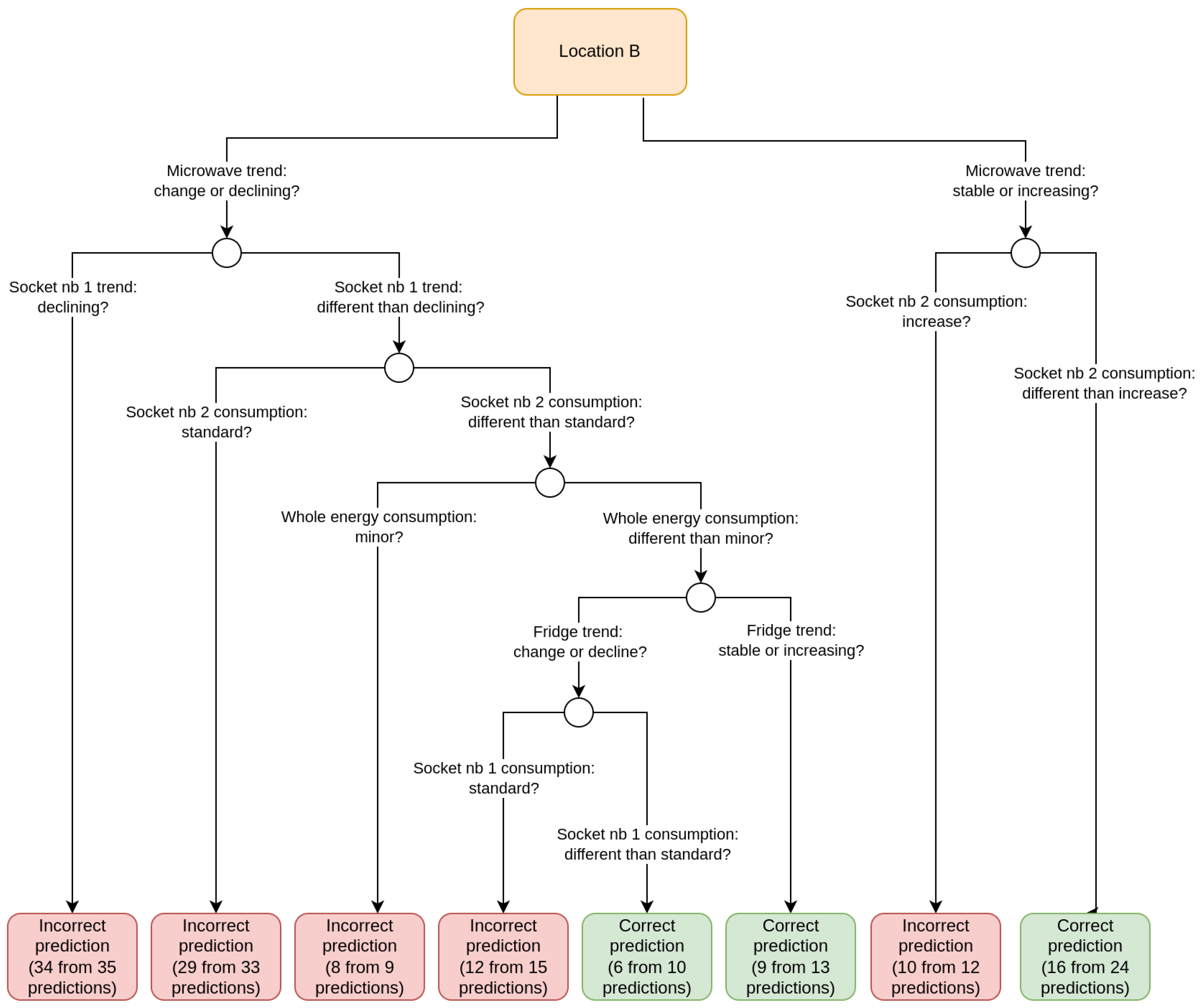
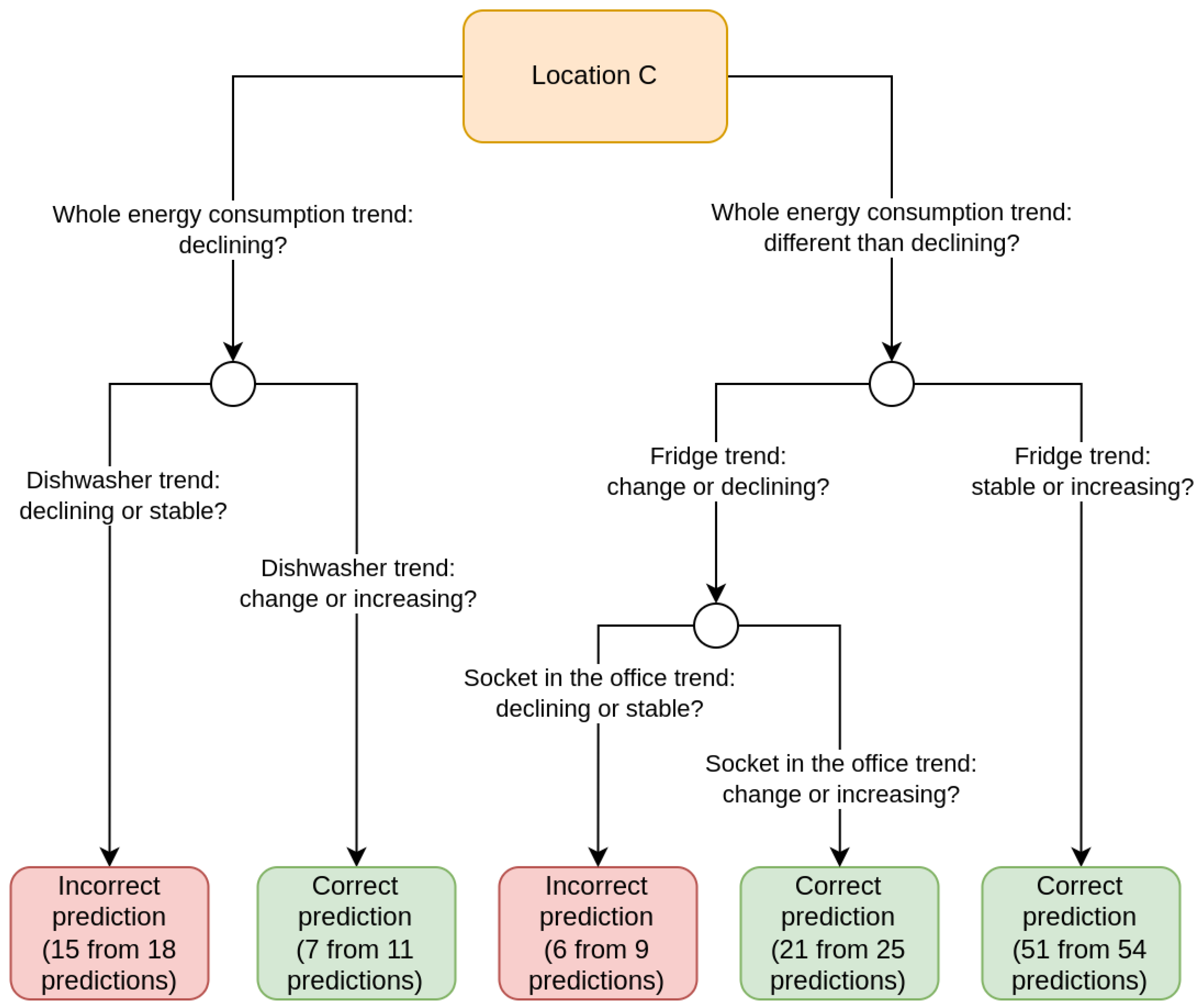
3.1. Analysis of Made Mistakes

As mentioned before, the acceptable error was below 25%. We wanted to check in which situations the best approach—devices_prophet—for each location made mistakes > 25%. We wanted to check if we could find any pattern in when models make good or bad predictions. This information could be treated as a knowledge discovery task that would help us understand the model. On the other hand, it could also be used as an additional input to the model, which could correct the predictions.

In order to do this, we designed a classification task to describe the situation in which the model was able to give satisfactory predictions (with error below 25%) and when the model was not able to do this. For each location and its devices_prophet model, we marked the prediction as Correct when the error for the prediction was below 25%, and Incorrect when the error for the prediction was equal or greater than 25% or the model did not give any prediction. This was treated as two labels in our classification task. Then, we created attributes that could describe how energy was consumed on a given day. We wanted to analyse if the consumption for the whole location was unusual and if the consumption for the specific device from the top 10 energy-consuming devices was uncommon. In order to analyse these situations, for the whole energy-consumption and for each device, we created the decision attribute that described the energy usage comparing with the consumption from different days (from a whole dataset). We distinguished five different situations:

• Consumption was minor—the consumption was in the range $(-\infty ,{\mu }_x-{\sigma }_x)$, where ${\mu }_x$ is the mean value of the time series x and ${\sigma }_x$ is the standard deviation of the time series x. Time series x is the time series describing 14 days before the day for which the attribute value was determined.
• There was a decrease in consumption—the consumption was in the range
  $({\mu }_x-{\sigma }_x,{\mu }_x-\frac{1}{2}{\dot{\sigma }}_x]$.
• The consumption was standard—the consumption was in the range
  $({\mu }_x-\frac{1}{2}{\dot{\sigma }}_x,{\mu }_x+\frac{1}{2}{\dot{\sigma }}_x]$.
• There was an increase in consumption—the consumption was in the range
  $({\mu }_x+\frac{1}{2}{\dot{\sigma }}_x,{\mu }_x+{\sigma }_x]$.
• The consumption was intense—the consumption was in the range
  $({\mu }_x+{\sigma }_x,\infty )$.

Then we created another set of attributes. They described the change of a trend of the time series. We distinguished five different situations of trend change:

• The trend was stable—the current consumption and the consumption for the day before were described as “standard”.
• The trend was declining—the current consumption and the consumption for the day before were described as “minor” or “decrease”.
• The trend was increasing—the current consumption and the consumption for the day before were described as “increase” or “intense”.
• There was a change in the trend—the current consumption was described differently than the consumption for the day before.

It is worth recalling that for each attribute describing the energy consumption of a location, two variables were created—one descriptively describing the energy consumption compared to the energy consumed in the last 14 days and a second variable describing a trend in energy consumption. For the devices_prophet model, there were 11 attributes that were time series: 1 feature described the total energy consumption and 10 features described the energy consumption of 10 devices. It means that a dataset with 22 conditional attributes was used to create a new decision model to determine when the model makes errors.

For the decision model, we used decision trees and their implementation in the rpart library that is available in R language. We discuss the results for two locations: B and C. We chose them because they represent different effectivenesses of devices_prophet models. For the location B, the Prophet model gave the worse results among the locations considered (MAPE was equal to 43.90%). For the location C, the Prophet model gave relatively good results (MAPE was equal to 18.17%). The generated decision models are presented in Figure 3 and Figure 4. The decision tree for location B had a balanced accuracy equal to 0.80 and the decision tree for location C had the balanced accuracy equal to 0.79. Balanced accuracy was calculated on the whole dataset.

The balanced accuracy of both trees shows that it is possible to find some patterns that describe at which points the Prophet model was wrong and at which points it gave good enough predictions. Some patterns can be difficult to interpret clearly, e.g., it can be difficult for us to understand why the Prophet model for location C gave more bad predictions when the dishwasher trend was stable than when there was a change in the trend. Note, however, that the change in energy consumption and trend characteristics (new attributes) were based on a comparison with the consumption period of the last 14 days. The tree model was learning on the whole data, and it is worth remembering that the stable value over this 14-day period was not necessarily stable in our understanding in the context of the whole dataset.

We can also see that the decision model interpreting the Prophet predictions was much more complex for location B than for location C. The Prophet model for location B did not give satisfactory results, so it means that the model could not find very strong patterns in energy consumption in this location. The tree decision model also shows that the model made mistakes in many different situations, and was not so easy to find the patterns that the model could learn. In Figure 5 we can see the energy consumption time series for the whole location and for the devices that were mentioned in the decision tree model (Figure 3). We can see that the trends are not very stable, and because of this, the Prophet model probably could not make sufficiently satisfactory predictions.

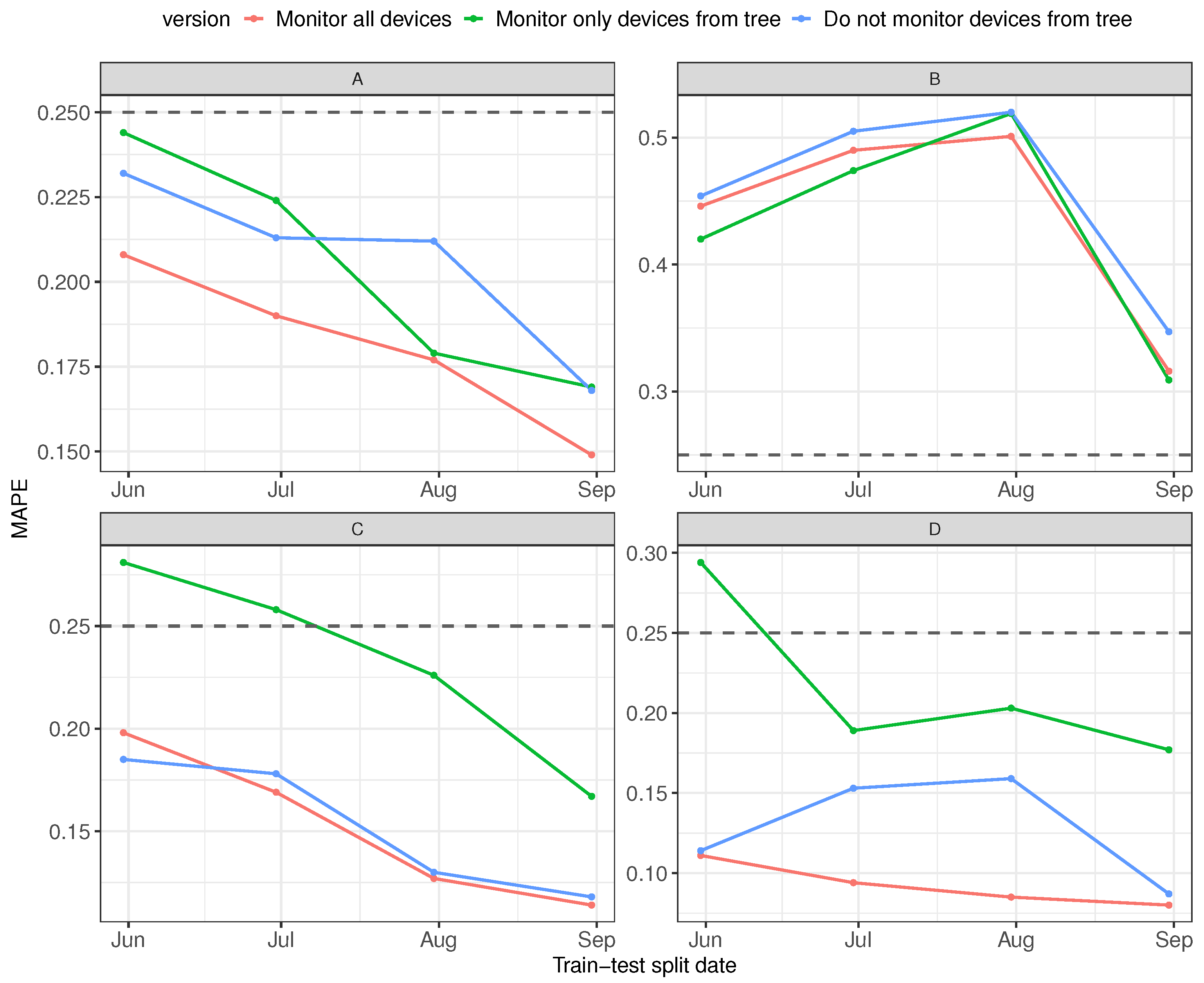
3.2. Limiting Number of Monitored Devices Based on Tree Decision Models

As shown in Section 3.1, the decision tree models with properly prepared attributes could satisfactory be used in order to describe the situations in which the main prediction model (in our case Prophet model) makes mistakes. The good quality of the models led us to consider whether the decision models might be able to help us reduce the number of devices monitored at the location.

It was already mentioned in the Introduction, that each measuring point consumes approximately 0.5–1 W, which, for 100 devices, increases the annual energy consumption to about 400 kWh. Furthermore, each measuring device costs money. Therefore, reducing the number of monitored devices is beneficial in terms of electricity consumption (paid for by the residents of the location) as well as the cost of purchasing new monitoring equipment (which the installer may buy).

We can imagine the situation that some monitored devices, even if they have large total energy consumption, may be irrelevant to the predictions because of their constant value of energy consumption or random consumption that could not be predicted by the Prophet model. We want to eliminate these kinds of devices from the monitored group. We checked how the device information obtained from the trees when the Prophet model makes mistakes could be useful to limit monitored devices.

We conducted the following experiments. Each dataset (for each location A, B, C, D) was divided into several train-test datasets. The pairs train-test were divided by the dates: “31 May 2021”, “30 June 2021”, “31 July 2021”, “31 August 2021”.

Thus, for each location, the first dataset was divided so that all data points before or equal “31 May 2021” were in the train dataset, and the rest were in the test dataset. The second pair was in the train dataset with data points before “1 July 2021”, and the rest was the test data, and so on. In this way, we obtained 16 test cases (four train-test splits for four locations).

Having a single train-test set, we built a decision tree on a train dataset that described the moments when the Prophet model made mistakes. The conditional attributes were created as for the trees in Section 3.1, i.e., there were features describing the change in energy consumption values as well as the trend, while the decision value was whether the model made an error >25% or not. Then on the test part, we studied two cases:

• How will the Prophet model perform on the test part when we use only the time series of the appliances whose features appeared in the decision tree and the time series describing the total energy consumption of the location to build a new model?
• How will the Prophet model perform on the test part when we do not use the time series of appliances whose features appeared in the decision tree?

Additionally, we investigated the predictions on the test set when all 10 appliances were used in building the model.

For each experiment, we built a decision tree for each date in a train dataset and ultimately used the last tree that had a Ballance Accuracy (BACC) ≥ 0.8 and the tree height was greater than 1. That is, for example, if the split between train and test set was for the date 31 August 2021 and the last tree that met the above conditions was built for the set for dates earlier than 20 August 2021, we used the tree built 20 August 2021 and not the one built 31 August 2021.

Therefore, for example, for location “A” we split the set at the beginning so that the last date of the training set was 31 May 2021. The rest of the set was the test set. The idea here is that on the data from March to 31 May 2021 we monitor the total energy consumption for the whole location, and we monitor these 10 devices. After that time, we generate a tree, and the installer removes monitoring for those devices that appeared in the tree, or we leave for further monitoring only those devices that appeared in the tree (these are the two versions of experiments). The third variant was when we did not change anything and continued monitoring the 10 devices in the Prophet model. Then, for this location, we did the same for the train-test split by date 30 June 2021, then 31 July 2021 and 31 August 2021. Note that for each split, the test set was different.

The results of using the proposed decision trees in order to limit the number of monitored devices are presented in Figure 6. For each location and each split date, the results of MAPE are presented. Because the test sets for each train-test split are different, we should not compare the MAPE values of the same version of the experiment for different threshold dates. Instead, we can compare how the three versions of the experiments came out, for each location and each train-test split date.

We can see that in most cases, the version of the experiment where we removed the information about the devices that appeared in the tree from the Prophet model gave results very close to when we monitored 10 devices. The results for location B can be ignored, because for it, the Prophet model did not perform well from the start. In the graphs, we have marked with a dashed line our error threshold, which is 25%. We can see that for locations A, C and D, the errors are below this threshold.

In

Table 5. The number of unique devices that appeared in the decision trees for each location and each split date.

	Location A	Location B	Location C	Location D
31 May 2021	4	1	2	3
30 June 2021	5	3	3	4
31 July 2021	4	3	4	4
31 August 2021	4	6	5	4

we present the number of devices that appeared in the decision trees for each location and each split date. We observe that for each case, at least one device was included in the tree, and it never happened that all devices appeared in the decision tree. The median of unique devices in the tree was 4, the mean was 3.7 and the maximum value was 6. Translating this to our problem of reducing the number of monitored devices using the decision tree, we can say that we were always able to remove at least one device from the observations, and it never happened that the tree indicated a recommendation to remove monitoring of all devices. The maximum number of devices removed from monitoring was six, and in most cases it did not exceed four devices. Such recommendations seem reasonable and not too extreme.

To summarize this part from a practical point of view: if an installer wanted to forecast the energy consumption of a location, they would start by monitoring the energy consumption of all N appliances in the location. Then, on the basis of this data, the Prophet model would be built, which would start forecasting the energy consumption for the following day. With the forecasts, we could assess on which days the Prophet model gave acceptable forecasts (below the assumed error) and when it did not. With information from a longer period of time, e.g., half a year, the installer could generate a decision tree that describes when the Prophet model makes unacceptable mistakes. Devices whose characteristics would be found in the decision tree would be removed from further monitoring, resulting in only M devices being monitored, where $M\le N$. If $M<N$, then the residents are saving money (because they do not pay for the energy consumption of $(N-M)$ sensors) and for the installer, who can use $(N-M)$ sensors in another location.

4. Discussion

Our research has shown that adding data on the energy consumption of the 10 most energy-intensive devices improves the results of the energy demand forecast for the following day. Energy consumption data for the appliances has a greater impact on prediction performance than weather forecast data. In the literature, we can find a lot of research dedicated to forecasting the daily energy demand in non-residential buildings. In the paper [42], we can see that the MAPE results for compared algorithms were 3.11–5.45%, with the lower error obtained for the support vector regression (SVR) model. The authors of [43] present the results obtained for an Artificial Neural Network (ANN) with MAPE 3.5–9.00%. In paper [44], the authors present an ensemble of various neural networks for prediction of heating energy consumption. In their research, they obtained MAPE errors of 5.25–5.43%. The MAPE results presented in [42,43,44] are lower than the results presented in this paper; however, the mentioned articles considered the non-residential buildings. Predicting the energy consumption in non-residential buildings is less complex than in residential buildings because of the relatively lower variability of occupant behaviour [45]. Because of this, the errors presented in the article can be higher than in the works based on data from commercial buildings. Forecasting the day-ahead energy usage in a residential building was presented in [46] with MAPE 12.36% for the multiple linear regression. It is important to point out that the results were obtained for 3 years of data, where our results were obtained for less than 6 months of data. As mentioned in the review [37], current research about data-driven building energy consumption was performed with various: types of data (real, simulated), granularities, types of buildings and sets of features. Because of this, it is difficult to compare the results with different papers. Additionally, only 19% of the studies reviewed in [37] focused on residential buildings. In the analysed papers, we also did not find work where real data about energy usage of the appliances in residential buildings were used to forecast the overall energy in the location. Because of this, we find our work novel and interesting for further development in the field.

In our research, we showed that the Prophet algorithm can be successfully used to forecast the energy demand in residential buildings. As far as we know, this method has not yet been presented in this field. Using an appropriate set of features, the Prophet model can give better results than the LSTM method. In the literature, we did not find a comparison of these two methods in the aspect of energy predictions.

We found some limitations of our research that we want to address. The study was performed for a few locations and for a limited period of time (the dataset did not cover the whole year). These limitations are a direct result of the fact that the research was carried out as part of a project. The number of monitored residential buildings within the project was limited due to the need to sensor multiple devices, which generated costs. This project ended in October 2021 and therefore the data collected does not cover the whole year. However, the limited dataset should not affect the reliability of the results, as the results presented were derived from a model that was retrained daily. This means that the model was re-learning as new data came in, so if the characteristics of the time series change, the model should adapt to the changing data.

Another limitation of the proposed solution is the cost of creating the digital-twin model of the building. This model assumes the observation of the energy consumption of many appliances used in the house, which generates the cost of purchasing sensors. However, our predictive model assumes the use of only information from the 10 most energy intensive appliances. In addition, we proposed a method for minimizing the number of monitored devices in the future.

5. Conclusions

Our research looks at how daily electricity consumption can be forecast for the next day, particularly in the context of a digital-twin model of a building.

First, our research has shown that monitoring energy consumption not only for an entire location, but also for selected appliances, can significantly improve the ability to predict future energy usage. Energy consumption data for the top 10 most energy-intensive appliances has a greater impact on prediction performance than weather forecast data.

Secondly, we have shown that the Prophet model, using the right dataset, gives (in most cases) the best results for predicting energy consumption for the next day. This method gave better forecast values than the LSTM neural network model and simple forecasting methods such as a naive model forecasting the value of the week before, and linear regression. An additional plus of Prophet is that it can easily be used by companies that do not have a large Data Science background. To the best of our knowledge, Prophet has never yet been described in the literature as a method for forecasting electricity demand, so the results data may be interesting in the context of further research work in this area.

Third, we have shown how model errors can be interpreted. Such knowledge can be used for future model corrections and to understand what activities of residents may affect the model forecast. The decision models also show which features (use of which devices) affect the forecast performance the most. This may indicate that these appliances are sometimes used in unpredictable ways, causing the model to fail to learn the energy consumption pattern of that appliance.

Last but not least, we used the proposed decision tree models describing the situations in which Prophet model makes a mistake, in order to limit the number of monitored devices. Devices whose features appeared in the tree would be removed. Removing these device data from the Prophet model gave, in most cases, MAPE results similar to those obtained when information about all devices was used in the Prophet model. By leaving only these devices and removing the others, we have seen a significant drop in forecast performance. We assume that such results are due to the fact that the devices that appear in the decision trees have a large variance of energy consumption and therefore are not useful for the Prophet model. The reduction of monitored appliances can be beneficial in reducing the energy consumption of the monitoring sensors themselves. Removed sensors can also be reused in other locations, generating savings. We assume that in order to validate the approach in more detail, a minimum dataset of one year would be needed to observe the characteristics of device use for the entire year. There were no data describing winter in our dataset and this could change the results obtained. We believe that it would be best to generate a tree for the whole year’s data.

To sum up: in our research, the proposed Prophet model, which uses information about the total energy consumption and the energy consumption of the top 10 energy-consuming devices, gave the best results for three out of four locations. For these three locations, the MAPE was below 25%, which was the error threshold which we have found to be acceptable. For this reason, we consider our research to have been successful at this stage. Future research will focus on the problem of using decision models, which interprets Prophet model errors, to improve forecast quality.

References

1. Zielińska-Sitkiewicz, M.; Chrzanowska, M.; Furmańczyk, K.; Paczutkowski, K. Analysis of Electricity Consumption in Poland Using Prediction Models and Neural Networks. Energies 2021, 14, 6619. [Google Scholar] [CrossRef]
2. Czosnyka, M.; Wnukowska, B.; Karbowa, K. Electrical energy consumption and the energy market in Poland during the COVID-19 pandemic. In Proceedings of the 2020 Progress in Applied Electrical Engineering (PAEE), Koscielisko, Poland, 21–26 June 2020; pp. 1–5. [Google Scholar] [CrossRef]
3. Jadwiszczak, P.; Jurasz, J.; Kaźmierczak, B.; Niemierka, E.; Zheng, W. Factors Shaping A/W Heat Pumps CO2 Emissions—Evidence from Poland. Energies 2021, 14, 1576. [Google Scholar] [CrossRef]
4. Alkhraijah, M.; Alowaifeer, M.; Alsaleh, M.; Alfaris, A.; Molzahn, D.K. The Effects of Social Distancing on Electricity Demand Considering Temperature Dependency. Energies 2021, 14, 473. [Google Scholar] [CrossRef]
5. Ozcanli, A.K.; Yaprakdal, F.; Baysal, M. Deep learning methods and applications for electrical power systems: A comprehensive review. Int. J. Energy Res. 2020, 44, 7136–7157. [Google Scholar] [CrossRef]
6. O’Dwyer, E.; Pan, I.; Charlesworth, R.; Butler, S.; Shah, N. Integration of an energy management tool and digital twin for coordination and control of multi-vector smart energy systems. Sustain. Cities Soc. 2020, 62, 102412. [Google Scholar] [CrossRef]
7. Walther, J.; Weigold, M. A Systematic Review on Predicting and Forecasting the Electrical Energy Consumption in the Manufacturing Industry. Energies 2021, 14, 968. [Google Scholar] [CrossRef]
8. Nowy System Rozliczania, Tzw. Net-Billing. Available online: https://www.gov.pl/web/klimat/nowy-system-rozliczania-tzw-net-billing (accessed on 30 May 2022).
9. Markakis, E.K.; Nikoloudakis, Y.; Lapidaki, K.; Fiorentzis, K.; Karapidakis, E. Unification of Edge Energy Grids for Empowering Small Energy Producers. Sustainability 2021, 13, 8487. [Google Scholar] [CrossRef]
10. Khajavi, S.H.; Motlagh, N.H.; Jaribion, A.; Werner, L.C.; Holmström, J. Digital Twin: Vision, Benefits, Boundaries, and Creation for Buildings. IEEE Access 2019, 7, 147406–147419. [Google Scholar] [CrossRef]
11. Reinhardt, H.; Bergmann, J.P.; Münnich, M.; Rein, D.; Putz, M. A survey on modeling and forecasting the energy consumption in discrete manufacturing. Procedia CIRP 2020, 90, 443–448. [Google Scholar] [CrossRef]
12. Erdogdu, E. Electricity demand analysis using cointegration and ARIMA modelling: A case study of Turkey. Energy Policy 2007, 35, 1129–1146. [Google Scholar] [CrossRef] [Green Version]
13. Wang, Y.; Wang, J.; Zhao, G.; Dong, Y. Application of residual modification approach in seasonal ARIMA for electricity demand forecasting: A case study of China. Energy Policy 2012, 48, 284–294. [Google Scholar] [CrossRef]
14. Tso, G.K.; Yau, K.K. Predicting electricity energy consumption: A comparison of regression analysis, decision tree and neural networks. Energy 2007, 32, 1761–1768. [Google Scholar] [CrossRef]
15. Bianco, V.; Manca, O.; Nardini, S. Linear Regression Models to Forecast Electricity Consumption in Italy. Energy Sources Part B Econ. Plan. Policy 2013, 8, 86–93. [Google Scholar] [CrossRef]
16. Ciulla, G.; D’Amico, A. Building energy performance forecasting: A multiple linear regression approach. Appl. Energy 2019, 253, 113500. [Google Scholar] [CrossRef]
17. Hong, T.; Gui, M.; Baran, M.E.; Willis, H.L. Modeling and forecasting hourly electric load by multiple linear regression with interactions. In Proceedings of the IEEE PES General Meeting, Minneapolis, MN, USA, 25–29 July 2010; pp. 1–8. [Google Scholar] [CrossRef]
18. Amber, K.P.; Aslam, M.W.; Mahmood, A.; Kousar, A.; Younis, M.Y.; Akbar, B.; Chaudhary, G.Q.; Hussain, S.K. Energy Consumption Forecasting for University Sector Buildings. Energies 2017, 10, 1579. [Google Scholar] [CrossRef] [Green Version]
19. Marino, D.L.; Amarasinghe, K.; Manic, M. Building energy load forecasting using Deep Neural Networks. In Proceedings of the IECON 2016—42nd Annual Conference of the IEEE Industrial Electronics Society, Florence, Italy, 23–26 October 2016; pp. 7046–7051. [Google Scholar] [CrossRef] [Green Version]
20. Kim, J.Y.; Cho, S.B. Electric Energy Consumption Prediction by Deep Learning with State Explainable Autoencoder. Energies 2019, 12, 739. [Google Scholar] [CrossRef] [Green Version]
21. Borghini, E.; Giannetti, C.; Flynn, J.; Todeschini, G. Data-Driven Energy Storage Scheduling to Minimise Peak Demand on Distribution Systems with PV Generation. Energies 2021, 14, 3453. [Google Scholar] [CrossRef]
22. Alhussein, M.; Aurangzeb, K.; Haider, S.I. Hybrid CNN-LSTM Model for Short-Term Individual Household Load Forecasting. IEEE Access 2020, 8, 180544–180557. [Google Scholar] [CrossRef]
23. Bouktif, S.; Fiaz, A.; Ouni, A.; Serhani, M.A. Multi-Sequence LSTM-RNN Deep Learning and Metaheuristics for Electric Load Forecasting. Energies 2020, 13, 391. [Google Scholar] [CrossRef] [Green Version]
24. Yan, K.; Li, W.; Ji, Z.; Qi, M.; Du, Y. A Hybrid LSTM Neural Network for Energy Consumption Forecasting of Individual Households. IEEE Access 2019, 7, 157633–157642. [Google Scholar] [CrossRef]
25. Koltsaklis, N.; Panapakidis, I.P.; Pozo, D.; Christoforidis, G.C. A prosumer model based on smart home energy management and forecasting techniques. Energies 2021, 14, 1724. [Google Scholar] [CrossRef]
26. Bu, S.J.; Cho, S.B. Time series forecasting with multi-headed attention-based deep learning for residential energy consumption. Energies 2020, 13, 4722. [Google Scholar] [CrossRef]
27. Braulio-Gonzalo, M.; Bovea, M.D.; Jorge-Ortiz, A.; Juan, P. Contribution of households’ occupant profile in predictions of energy consumption in residential buildings: A statistical approach from Mediterranean survey data. Energy Build. 2021, 241, 110939. [Google Scholar] [CrossRef]
28. Song, S.Y.; Leng, H. Modeling the household electricity usage behavior and energy-saving management in severely cold regions. Energies 2020, 13, 5581. [Google Scholar] [CrossRef]
29. Sepehr, M.; Eghtedaei, R.; Toolabimoghadam, A.; Noorollahi, Y.; Mohammadi, M. Modeling the electrical energy consumption profile for residential buildings in Iran. Sustain. Cities Soc. 2018, 41, 481–489. [Google Scholar] [CrossRef]
30. Beaudin, M.; Zareipour, H. Home energy management systems: A review of modelling and complexity. Renew. Sustain. Energy Rev. 2015, 45, 318–335. [Google Scholar] [CrossRef]
31. Sharma, V.; Cortes, A.; Cali, U. Use of Forecasting in Energy Storage Applications: A Review. IEEE Access 2021, 9, 114690–114704. [Google Scholar] [CrossRef]
32. Deb, C.; Zhang, F.; Yang, J.; Lee, S.E.; Shah, K.W. A review on time series forecasting techniques for building energy consumption. Renew. Sustain. Energy Rev. 2017, 74, 902–924. [Google Scholar] [CrossRef]
33. Almazrouee, A.I.; Almeshal, A.M.; Almutairi, A.S.; Alenezi, M.R.; Alhajeri, S.N. Long-Term Forecasting of Electrical Loads in Kuwait Using Prophet and Holt–Winters Models. Appl. Sci. 2020, 10, 5627. [Google Scholar] [CrossRef]
34. Bashir, T.; Haoyong, C.; Tahir, M.F.; Liqiang, Z. Short term electricity load forecasting using hybrid prophet-LSTM model optimized by BPNN. Energy Rep. 2022, 8, 1678–1686. [Google Scholar] [CrossRef]
35. Vartholomaios, A.; Karlos, S.; Kouloumpris, E.; Tsoumakas, G. Short-Term Renewable Energy Forecasting in Greece Using Prophet Decomposition and Tree-Based Ensembles. In Database and Expert Systems Applications—DEXA 2021 Workshops; Springer: Cham, Switzerland, 2021; pp. 227–238. [Google Scholar] [CrossRef]
36. Hasan Shawon, M.M.; Akter, S.; Islam, M.K.; Ahmed, S.; Rahman, M.M. Forecasting PV Panel Output Using Prophet Time Series Machine Learning Model. In Proceedings of the 2020 IEEE REGION 10 CONFERENCE (TENCON), Osaka, Japan, 16–19 November 2020; pp. 1141–1144. [Google Scholar] [CrossRef]
37. Amasyali, K.; El-Gohary, N.M. A review of data-driven building energy consumption prediction studies. Renew. Sustain. Energy Rev. 2018, 81, 1192–1205. [Google Scholar] [CrossRef]
38. Prophet. Prophet, Forecasting at Scale. Available online: https://facebook.github.io/prophet/ (accessed on 3 May 2022).
39. Punia, S.; Nikolopoulos, K.; Singh, S.P.; Madaan, J.K.; Litsiou, K. Deep learning with long short-term memory networks and random forests for demand forecasting in multi-channel retail. Int. J. Prod. Res. 2020, 58, 4964–4979. [Google Scholar] [CrossRef]
40. Hundman, K.; Constantinou, V.; Laporte, C.; Colwell, I.; Soderstrom, T. Detecting Spacecraft Anomalies Using LSTMs and Nonparametric Dynamic Thresholding. In Proceedings of the 24th ACM SIGKDD International Conference on Knowledge Discovery & Data Mining, London, UK, 19–23 August 2018; Association for Computing Machinery: New York, NY, USA, 2018. KDD ’18. pp. 387–395. [Google Scholar] [CrossRef] [Green Version]
41. Taylor, S.J.; Letham, B. Forecasting at Scale. Am. Stat. 2018, 72, 37–45. [Google Scholar] [CrossRef]
42. Fan, C.; Xiao, F.; Wang, S. Development of prediction models for next-day building energy consumption and peak power demand using data mining techniques. Appl. Energy 2014, 127, 1–10. [Google Scholar] [CrossRef]
43. Jetcheva, J.G.; Majidpour, M.; Chen, W.P. Neural network model ensembles for building-level electricity load forecasts. Energy Build. 2014, 84, 214–223. [Google Scholar] [CrossRef]
44. Jovanović, R.Ž.; Sretenović, A.A.; Živković, B.D. Ensemble of various neural networks for prediction of heating energy consumption. Energy Build. 2015, 94, 189–199. [Google Scholar] [CrossRef]
45. Jain, R.K.; Smith, K.M.; Culligan, P.J.; Taylor, J.E. Forecasting energy consumption of multi-family residential buildings using support vector regression: Investigating the impact of temporal and spatial monitoring granularity on performance accuracy. Appl. Energy 2014, 123, 168–178. [Google Scholar] [CrossRef]
46. Iwafune, Y.; Yagita, Y.; Ikegami, T.; Ogimoto, K. Short-term forecasting of residential building load for distributed energy management. In Proceedings of the 2014 IEEE International Energy Conference (ENERGYCON), Cavtat, Croatia, 13–16 May 2014; pp. 1197–1204. [Google Scholar] [CrossRef]
Figure 1. Schema of the digital-twin model of a building.
Energies 15 04318 g001
Figure 2. Decomposition of energy consumption time-series for each location. Trend and weekly seasonality are presented.
Energies 15 04318 g002
Figure 3. Decision tree explaining when the device_prophet models made mistakes for location B.
Energies 15 04318 g003
Figure 4. Decision tree explaining when the device_prophet models made mistakes for location C.
Energies 15 04318 g004
Figure 5. Time series for the whole energy consumption in location B and time series for the devices and attributes used in the decision tree (Figure 3)—microwave, fridge, socket number 1, socket number 2.
Energies 15 04318 g005
Figure 6. Value of mean absolute percentage error (MAPE) for locations (AD) and each split date for train-test datasets. The dashed line indicates the maximum error threshold—25%.
Energies 15 04318 g006