Abstract
As many new devices and factors, such as renewable energy sources, energy storage (ESs), electric vehicles (EVs), and demand response (DR), flood into the distribution network, the characteristics of the distribution network are becoming complicated and diversified. In this study, a two-layer collaborative optimized operation model for the multi-character distribution network considering multiple uncertain factors is proposed to achieve optimal dispatching of ES and EV and obtain the optimal grid structure of the distribution network. Based on basic device models of distribution network, the upper layer distribution network reconfiguration (DNR) model is established and solved by the particle swarm optimization (PSO) based on the Pareto optimality and the Prim algorithm. Then, the lower layer optimal dispatching model of ES and EV is established and solved by the binary PSO. The upper layer model and the lower layer model are integrated to form the collaborative optimized operation model for the multi-character distribution network and solved by iterating the upper and lower layers continuously. A case study is conducted on the IEEE 33-bus system. The simulation results show that the total network loss and the voltage deviation are decreased by 15.66% and 15.52%, respectively, after optimal dispatching of ES and EV. The total network loss and the voltage deviation are decreased by 28.39% and 44.46%, respectively, after the DNR with distributed generation (DG) and EV loads with little impact on the average reliability of the power supply. The total network loss and the voltage deviation are decreased by 26.54% and 27.04%, respectively, after the collaborative optimized operation of the multi-character distribution network. The collaborative optimized operation of the distribution network can effectively reduce the total cost by 114.45%, which makes the system change from paying to gaining.
1. Introduction
With the increasing access to ES, EV, and renewable energy generation devices such as wind turbines and photovoltaics, the distribution network is becoming a multi-character system. The access of these devices will bring a series of influences on the distribution network, including changing the power flows of the system, affecting the frequency and voltage of the network, and so on. Therefore, it is of great economic and safety benefit to analyze the characteristics and establish mathematical models of these devices to further study the optimal operation of the distribution network. The key technologies of the multi-character distribution network are DNR and optimal dispatching of ES and EV. A large number of domestic and foreign scholars have already completed research on these aspects.
Several studies have been conducted on establishing the DNR model. The consumption of DG in the objective function in [1] is maximized as much as possible while satisfying the security constraints. The multi-objective game model in [2] solves the issue of ignoring the relationship between objectives. In [3], a dynamic DNR model which accounts for the three-phase asymmetry of the distribution network and the imbalance degree constraint of DG is constructed. A mixed-integer non-linear DNR optimization model is proposed in [4], aiming to minimize active power losses. The microgrid-based DNR is analyzed by taking DR and power-sharing into account to optimize costs and reduce power losses [5]. A practical DNR case study of an 11 kV distribution network that feeds residential rural loads in middle Egypt is modeled and analyzed in [6]. The harmony search algorithm is presented for avoiding infeasible solutions during the DNR in [7] and is applied to the practical 10 kV distribution network in a city in south China.
The intelligent algorithm is the most widely used method to solve DNR models for its strong ability in optimization. The DNR problem is solved by a selective bio-inspired metaheuristic based on microbats’ behavior named the selective bat algorithm together with the EPRI-OpenDSS software (California, US, EPRI) in [8]. An improved harmony search algorithm is proposed in [4] to solve the DNR problem, whose main novelty is the inclusion of a path relinking phase which accelerates the convergence of the reconfiguration problem. The shade optimization algorithm along with the SOE reconfiguration method has been employed in [9] to solve the optimization problem with consideration of the uncertainty of the network load and the output power of renewable DGs. The improved two-particle swarm optimization algorithm in [10] is proposed to solve the multi-objective nonlinear optimization problem. A distributed PSO based on the Hadoop platform is proposed in [11] to find an optimal solution to a high dimension optimization problem. An improved artificial fish swarm algorithm that improves the flexibility of the algorithm in the process of DNR is proposed in [12]. Reconfiguration coding rules are combined with the improved firefly algorithm to achieve fast DNR in [13].
In terms of the optimization of ES and EV, ES capacity is optimized by a two-layer optimization model that includes the charge/discharge optimal dispatching of ES in [14]. The optimal dispatching strategy of the ES system is proposed by taking the battery life and the state of charge into account [15]. An optimal dispatching model of ES with the objectives of minimizing load fluctuations in the voltage deviation is established in [16]. As for the optimal dispatching of EV, a dispatching strategy for EV considering characters of mobile ES is proposed in [17]. The two-layer plan model to optimize the charge/discharge dispatching operation of EV is developed [18]. A real-time dispatching model with the objectives of minimizing power fluctuations and charge/discharge cost is established in [19]. Other important factors should be taken into account, such as DR. A two-stage ES sharing mechanism considers DR to provide reliable resources for real-time optimization and applied the model to the Pennsylvania–New Jersey–Maryland electricity market [20]. An investigation is made in [21], focusing on the energy DR actions on energy consumption and cost for a thermal energy storage system with a ground source heat pump in a detached residential house in a cold climate. The influence of DR actions on thermal comfort and electricity cost in residential buildings with different heating systems in Finland is studied in [22].
The proposed models and theories of this paper have important value in practical application. DNR can be used to solve many distribution network problems. For example, the distribution network with DG sources may face the problem that some load points cannot be restored to power during the fault recovery process. Therefore, the DNR can be combined with the islanding operation to form the distribution network fault recovery strategy [5]. What is more, DNR, as an active management measure, can be combined with a reactive power optimization strategy to solve optimization problems. EV and ES are flexible factors in the distribution network. The experience of power system operation in Europe shows that with an adequate and effective dispatching strategy, the investment cost of renovation and expansion of the network can be reduced by more than half. In addition, for active distribution networks, effective network optimization and scheduling strategies can improve the utilization of renewable energy and reduce power losses [16]. Moreover, EV clusters can be used as ES modules to smooth power fluctuation of distributed renewable energy sources, thus achieving power coordination in all devices.
In order to analyze the collaborative optimized operation of the multi-character distribution network comprehensively, improve the efficiency and operation level of the network, and fully utilize the regulation ability of ES, EV, and DG to optimize the network operation, the two-layer collaborative optimized operation model for the multi-character distribution network considering multiple uncertain factors is proposed. The main contributions and novelties of this paper are summarized as follows:
- (1)
- The optimal dispatching model for ES and EV is proposed to realize the cooperation of ES and EV. Compared with the existing studies that only use optimal dispatching strategies to solve other problems of distribution networks, the proposed model takes ES and EV as indispensable parts of the system, thus fully releasing the adjustable potential of them.
- (2)
- The DNR model is proposed to obtain the optimal grid structure of the distribution network. In the process of multi-objective optimization of existing studies, when a single objective deviates from its expectation greatly, other objectives are easily ignored. The proposed DNR model can measure the importance of each objective function reasonably. Compared with the existing intelligent algorithms with a wide search range which leads to slow convergence, the combination of the Prim algorithm and the Pareto optimality can obtain the optimal solution of the multi objective problem with high accuracy and fast speed while making sure the topology of the generated grid structure is radical.
- (3)
- A two-layer collaborative optimized operation model of a multi-character distribution network is established based on the above two models, of which the optimal dispatching model for ES and EV is the lower layer and the DNR model is the upper layer. The collaborative optimized operation model takes all the factors and devices of the distribution network into consideration, including ES, EV, DG, and DR. The proposed model fills in the blanks of existing studies which usually do not consider all the factors of the distribution network.
The rest of the paper is organized as follows. Section 2 presents the basic device models of the distribution networks, including the DG models, the ES model, the EV model, and the DR model. In Section 3, the lower layer optimal dispatching model of ES and EV is explained; in Section 4, the upper layer DNR model is explained; in Section 5, the collaborative optimized operation model is explained; in Section 6, the results of the case study on the IEEE 33-bus system are discussed, and the conclusion is provided in Section 7.
2. Basic Device Models of Multi-Character Distribution Network
2.1. DG Output Model
The wind turbine output model [23] is shown in (1). The photovoltaic output model [24] is shown in (2)
where is the output power of wind turbine; is the rated output power; , and are the cut-in, cut-out, and rated wind speed; PPV is the output power of photovoltaic; is the number of photovoltaic cells; is the rated output power of a photovoltaic cell; and are the actual and rated light intensity; k is the power temperature coefficient; and are the actual and standard temperature.
2.2. Non-Dispatchable EV Load Model
The modes of EV access to the grid can be divided into two categories [25]: non-dispatchable mode (EV only absorb electricity from the grid for charging) and dispatchable mode (both charging/discharging, acting in the same way as ES devices). We divided EV into three categories: buses, taxis, and private cars, which follow different normal distributions. The daily power consumption of non-dispatchable EV is related to the daily mileage, which follows a normal distribution [23] shown in (3). Then we use (3) to sample each EV to obtain the daily mileage, and afterward calculate the SOC (battery state of charge) of it. According to daily power consumption, the time required for charging each day can be obtained by (6).
where is the daily mileage of EV; μ and σ are the mean value and standard deviation of and the normal distribution, is the daily power consumption of EV; is the maximum mileage; is the battery capacity of EV; is the remaining SOC of EV after driving ; is the total charge time that EV requires in a day; is the charge power of EV.
2.3. Charge/Discharge Model of ES and Dispatchable EV
The dispatchable EV has the same effort as ES and can be viewed as a larger capacity battery, so they can be described by the same model. The balance equations of charge/discharge energy [26] are shown in (7) and (8). The constraints for SOC and the charge/discharge power are shown in (9)–(11).
where is the energy stored in ES at moment t; η is the charge and discharge loss coefficient of ES; and are the charge and discharge power of ES. and are the upper and lower limits of SOC; and are the upper and lower limits of charge power; and are the upper and lower limits of discharge power.
2.4. DR Model
DR model considering electricity price and policy is shown in (12).
where is the per-unit load of node i at time t after DR; and are the demand elasticity coefficients of node i with respect to electricity price and policy; is the difference between electricity price and average electricity price at time t; a is the policy impact factor; and are the per-unit transferable load and per-unit non-transferable load of node i at time t.
3. Optimal Dispatching Model of ES and EV and Solving Algorithm
3.1. Objective Functions
We optimize the charging/discharging strategy for ES and dispatchable EV in a day to make sure the total cost is minimized. The objective function is shown in (13).
where M is the total number of ES and EV. is the cost of the number of charge/discharge operations, as there is an upper limit to the number of times a battery can be charged/discharged, so there is a cost for each charge/discharge operation. is the cost of charge/discharge power of the battery. The reason for this cost is that due to the peak and valley tariffs, the charge/discharge operation of the battery at different times will lead to an imbalance of revenue and expenditure. is the cost of wear and tear in a non-working state, which is due to the fact that the battery will age over time, even if it is not working. is the penalty cost after the battery enters the dead zone. The reason for this cost is that the battery can no longer charge/discharge after entering the dead zone, resulting in a decrease in the battery’s regulation of power flow. is the cost of total network loss throughout the day. is the cost of voltage deviation.
where and are the number of charge/discharge operations and the allowable number of charge/discharge operations of the ith device; is the battery cost of the ith device. is the electricity price at time t; is the charge/discharge power of the ith device at time t, whose value is positive when charging and negative when discharging. is the length of time that the ith device is not working; is the total life of the ith device. is the penalty cost per unit of time; is the total time that the ith device in the dead zone. is the active power loss of the network at time t; and are the active and reactive power of line kj at time t; is the voltage of node j at time t; is the resistance of line kj. is the cost factor of voltage deviation; is the amount of voltage deviation at node j at time t; J is the total number of nodes.
3.2. Constraint Conditions
The power balance constraints are shown in (20) and (21). The node voltage constraint is shown in (22). The line capacity constraint is shown in (23) The ES and EV constraints are shown in (9)–(11).
where and are injected active and reactive power of node i; and are the output active and reactive power from DG of node i; and are the active and reactive loads of node i; and are the load of ES and EV of node i; and are the conductance and susceptance of line ij; θij is the difference of voltage phase angle between the two ends of line ij; and are the actual and rated voltage of node i; Sij max is the maximum capacity allowed for line ij.
3.3. Optimization Strategies and Improvements of Solving Algorithm
The PSO [27] consists of updating formulas of velocity and position, which converge the positions of the particles to the global optimal position through continuous iterations.
where and are the velocity and position vectors of the kth iteration of the ith particle; ρ is the inertia coefficient; is the global optimal position; is the individual optimal position of the ith particle; and are the learning factors; r1 and r2 are random numbers within [0, 1].
The effective SOC range of the battery is from 20% to 80%, and when SOC reaches the boundary, the battery enters the dead zone, resulting in a significant reduction in the battery’s regulation of load. So, we adopted the dead time constraint strategy to limit the dead time, which is shown in (26). As the SOC approaches 80%, the velocity of the particle tends to be negative, and thus the position of the particle tends to be negative, increasing the discharging possibility of the device and reducing its SOC, and vice versa.
where is the original updating formula of velocity shown in (24); and are random numbers; is the SOC vector of the battery of the ith particle; β is a constant designed to prevent the denominator from reaching zero.
The role of ES and EV is to regulate the load and smooth power flow, so we proposed the charge/discharge power optimization strategy shown in (27) and (28) to improve the updating formula of velocity.
where is the updating formula of velocity shown in (26); is the learning factor; r5 is a random number within [0, 1]; is the average load; is the daily load; is the EV load; is the output power of DG.
According to the strategies mentioned above, the solving process of the optimal dispatching model of ES and EV is shown in Figure 1.
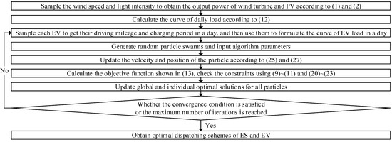
Figure 1.
Solving process of optimal dispatching model for ES and EV.
4. Distribution Network Reconfiguration Model and Solving Algorithm
4.1. Objective Functions
is the economy function described by the network power losses shown in (29). is the security function characterized by voltage offsets shown in (30).
where k is the branch number; B is the total number of branches; and are the active and reactive power flows of branch k; is the resistance of branch k; is the voltage at the first end of branch k. i is the node number; J is the total number of nodes.
4.2. Constraint Conditions
The power balance constraints [28] are shown in (31) and (32). The node voltage constraint and branch current constraint [29] are shown in (33) and (34). The reliability constraint of the network is shown in (35). The mathematical expression of network topology constraint [30] is shown in (36).
where and are the active and reactive power losses of the network; Ps and Qs are the active and reactive power injected into the distribution network by the root node. and are the upper and lower voltage limits of node i. is the current of branch k; is the maximum current allowed for branch k. ASAI is the average power supply availability; is the fault rate of branch k; is the active power outage caused by the fault of branch k; t is the average outage duration; is the lower limit of ASAI. and are the number of connected nodes and branches.
4.3. Solving Algorithm for Network Reconfiguration
We use a binary PSO based on the Prim algorithm [31] to solve the DNR model. The model is a multi-objective problem; therefore, the principle of Pareto optimality [32] is used to determine the optimal solution. Moreover, the Prim algorithm can make sure that the model generates a radial network structure, so there is no need to verify that the topology satisfies the open-loop condition.
The goal of network reconfiguration is to obtain the optimal grid structure. Each branch has two states, selected and unselected, which can be represented by the binary code 1 and 0, respectively. The position of a particle is a vector whose dimension equals the number of branches, and each dimension can only take on a value of 1 or 0. The updating equations of velocity and position are shown in (37)–(39).
where and are the velocity and position vectors of the ith particle in the kth iteration; is the individual optimal position of the ith particle after the kth iteration; is the global optimal position after the kth iteration; and are accelerating factors; and are the upper and lower limits of velocity in function S; is the position of the dth dimension of the ith particle in the kth iteration; is the velocity of the dth dimension of the ith particle in the k − 1th iteration; r is a random number within [0, 1].
The solving process of the DNR model is shown in Figure 2.
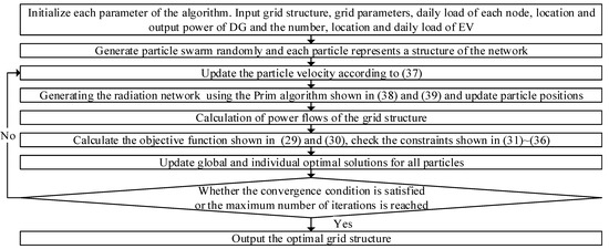
Figure 2.
Solving process of DNR model.
5. Collaborative Optimized Operation Model of Multi-Character Distribution Network
In this section, we combine the upper layer DNR model shown in Section 4 and the lower layer optimal dispatching model of ES and EV shown in Section 3 into a collaborative optimized operation model. The optimal solution can be obtained through continuous iteration between the upper and lower layers. The procedure of the algorithm is described below.
- (1)
- Initialize all the parameters. Input the load, power output of DG, parameters of EV, ES, and dispatchable EV, and grid information of each node for 24 h.
- (2)
- Calculate the injected power of each node, including the load, power output of DG, EV load, and charge/discharge power of ES and dispatchable EV.
- (3)
- Solve the upper layer DNR model using the binary PSO based on the Prim algorithm and output the optimal solution which represents the optimal grid structure when the condition of the Pareto optimal solution is met.
- (4)
- Pass the optimal grid structure of the upper layer to the lower layer optimization model.
- (5)
- Solve the lower layer optimization model using the PSO based on optimization strategies and output the optimal charge/discharge dispatching schemes of ES and EV in 24 h.
- (6)
- Determine whether the change of the objective function value of the lower-layer model between two iterations is less than the threshold value; if not, pass the output result of the lower-layer model to the upper-layer model and go to step (2); if yes, turn to step (7).
- (7)
- Output the charge/discharge dispatching schemes of ES and EV of 24 h and the optimal grid structure.
The solving process of collaborative optimized operation model of multi-character distribution network is shown in Figure 3.
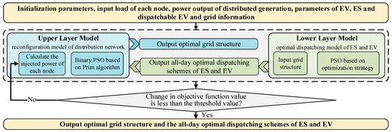
Figure 3.
Solving process of collaborative optimized operation model of multi-character distribution network.
6. Case Study
6.1. Basic Information of Example System
The proposed approach is implemented in MATLAB and tested on the IEEE 33-bus [33] system shown in Figure 4. The whole year is divided into four scenarios: spring, summer, autumn, and winter. The relevant system parameters are shown in Appendix A. The total active and reactive load of the system is 3.715 MW and 2.3 Mvar, respectively. The rated voltage is 12.66 kV.

Figure 4.
Grid structure of IEEE 33-bus system.
6.2. Optimal Dispatching of ES and EV
We use the optimal dispatching model of ES and EV to obtain the optimal dispatching schemes for four scenarios. The SOC results of ES and EV after the optimal dispatching in a day are shown in Figure 5.
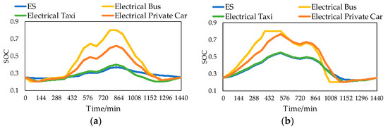
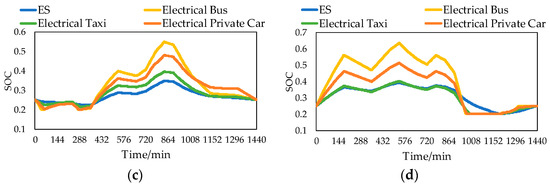
Figure 5.
SOC results of ES and EV. (a) Spring. (b) Summer. (c) Autumn. (d) Winter.
The load curve before and after optimal dispatching of ES and EV are shown in Figure 6. It can be seen from Figure 6 that the load after dispatching is significantly smoother than that before dispatching, and the peak-valley difference is significantly reduced. It is obvious that ES and dispatchable EV can smooth the load and reduce the peak-valley difference of load. This is due to the fact that when operating in the dispatchable mode, EVs can both absorb electricity from the grid and release electricity to the grid, acting in the same way as ES devices. ES devices can regulate the load, smooth the load and reduce power flow fluctuations through planned charge and discharge behavior, so the load after the dispatching of ES and EV is much smoother than before.
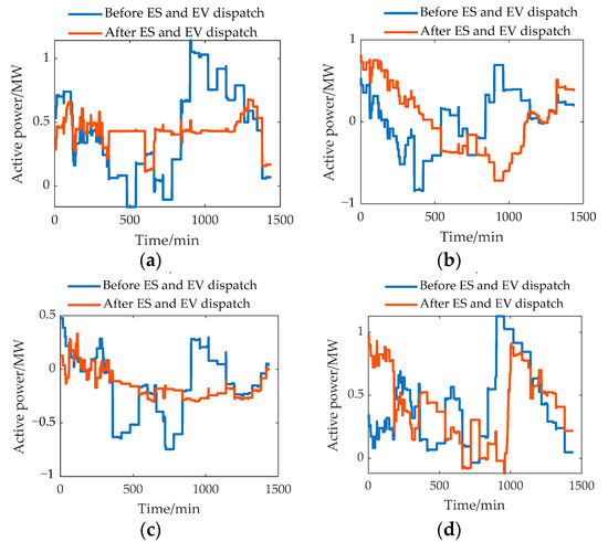
Figure 6.
Load curve before and after the dispatching of ES and EV. (a) Spring. (b) Summer. (c) Autumn. (d) Winter.
In order to further illustrate the importance of ES and dispatchable EV, we removed all the ES and dispatchable EV and solve the dispatching problem again. The comparison of results with and without ES and dispatchable EV are shown in Figure 7. The percentage of decrease in the total network loss and voltage deviation with ES and dispatchable EV is shown in Table 1. In all scenarios, the access of ES and dispatchable EV reduces the total network loss and voltage deviation. In spring, the comparison of the results with and without ES and dispatchable EV is the most obvious of the four scenarios. The total network loss is reduced by 23.58% and the voltage deviation is reduced by 50.56% in spring. After optimal dispatching of ES and EV, the percentage of decrease in the total network loss within the year is 15.66%, and the percentage of decrease in voltage deviation within the year is 15.52%. In summary, the optimal dispatching model of ES and EV can smooth the load, reduce network power loss, and increase voltage quality.
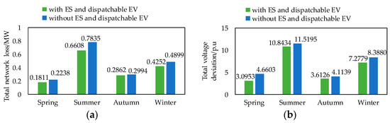
Figure 7.
Comparison of results with and without ES and dispatchable EV in multiple scenarios. (a) Total network loss. (b) Total voltage deviation.

Table 1.
The percentage of decrease in total network loss and voltage deviation after dispatching of ES and EV.
In order to verify the effectiveness of the dead time constraint strategy and the charge/discharge power optimization strategy proposed in Section 3.3, Table 2 shows the comparisons of the dispatching results of the spring scenario with or without each strategy.
Table 2.
The dispatching results of spring scenario with or without each strategy.
According to Table 2, when there is no dead time constraint, the total time the battery is in the dead zone and the total non-working time of the battery are significantly increased, which is nearly six times that when there is a dead time constraint. The decrease in the regulation effect of the battery leads to the weakening of effects of ES and dispatchable EV, resulting in an increase in total network loss and total voltage deviation for the whole day.
Figure 8 is the comparison of the load curve with and without the charge/discharge power optimization strategy. Combining Figure 8 with Table 2, when there is no charge/discharge power optimization strategy, the total load increases sharply, which is because the large charge/discharge power of ES and dispatchable EV is very large. At this time, the system cannot regulate load well and the battery is more likely to enter the dead zone and nonworking state.
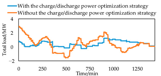
Figure 8.
Comparison of load curve with and without charge/discharge power optimization strategy.
6.3. Network Reconfiguration with DG and EV Loads
We use the DNR model to conduct simulations on each scenario. Optimized grid structures for each scenario are shown in Figure 9.
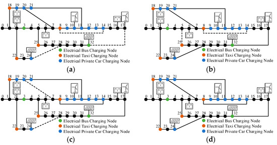
Figure 9.
Optimized grid structure for each scenario. (a) Spring. (b) Summer. (c) Autumn. (d) Winter.
Comparisons of results before and after reconfiguration are shown in Figure 10. The percentage of decrease in total network loss, voltage deviation, and average reliability of power supply after reconfiguration is shown in Table 3. It can be seen from Figure 10 and Table 3 that the total network loss and total voltage deviation after reconfiguration are reduced, and the reduction in voltage deviation is more obvious. After reconfiguration, the percentage of decrease in the total network loss within the year is 28.39%, and the percentage of decrease in voltage deviation within the year is 44.46%. In summer, the comparison of the results before and after the reconfiguration is the most obvious of the four scenarios. The total network loss is reduced by 38.96% and the total voltage deviation is reduced by 59.50% in summer.
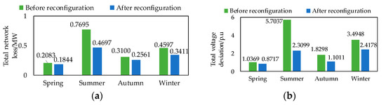
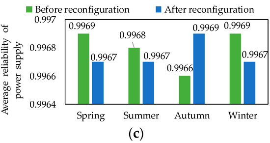
Figure 10.
Comparison of results before and after DNR. (a) Total network power loss. (b) Total voltage deviation. (c) Average reliability of power supply.
Table 3.
The percentage of decrease in total network loss, voltage deviation, and average reliability of power supply after reconfiguration.
The percentage of decrease in average reliability of power supply within the year is 0.01% in Table 2, which means the average reliability of power supply is not much different, that is because before and after reconfiguration, the topology of the distribution network is radial and the power supply mode is open-loop single power supply, so the reconfiguration has little impact on the reliability of power supply.
6.4. Collaborative Optimized Operation of Multi-Character Distribution Network
This section analyzes the collaborative optimization operation model of the multi-character distribution network of four seasons. A comparison of results between the optimized dispatching model and collaborative optimized operation model is shown in Figure 11. The percentage of decrease in the total network loss, voltage deviation, and total cost of collaborative optimized operation model of distribution network compared to optimal dispatching model for ES and EV is shown in Table 4.
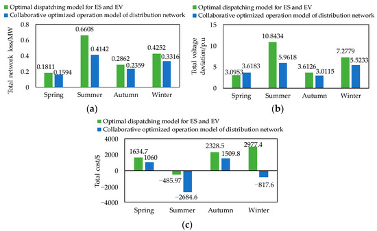
Figure 11.
Comparison of results between optimized dispatching model and collaborative optimized operation model. (a) Total network loss. (b) Total voltage deviation. (c) Total cost.
Table 4.
The percentage of decrease in total network loss, voltage deviation, and total cost of collaborative optimized operation model of distribution network compared to optimal dispatching model for ES and EV.
We can observe through Figure 11 and Table 4 that the results of the collaborative optimized operation model are better than that of the optimal dispatching model for almost all scenarios, with the most obvious difference in the results in summer. Compared with the optimal dispatching model, the total network loss calculated by the collaborative optimized operation model is reduced by 37.32%, the total voltage deviation is reduced by 45% and the total cost is reduced by 452.42%. Although the voltage deviation calculated by the collaborative optimized operation model at spring is slightly higher than that calculated by the optimal dispatching model, the total cost calculated by the collaborative optimized operation model is lower than that calculated by the optimal dispatching model, which is 35.16% lower.
In Table 4, the percentage of decrease in the total network loss within the year is 26.54%, the percentage of decrease in voltage deviation within the year is 27.04% and the percentage of decrease in total cost within the year is 114.45%. In summary, the collaborative optimized operation model can significantly reduce the total cost and improve the economy and safety of the distribution network compared with the optimal dispatching model of ES and EV.
7. Conclusions
This paper established a collaborative optimized operation model of a multi-character distribution network and solved it by the binary PSO. The collaborative optimized operation problem of the multi-character distribution network is decomposed into the optimal dispatching subproblem and the network configuration subproblem. The main conclusions are as follows:
- (1)
- Taking ES and EV into consideration, the optimal dispatching model can reduce the total network loss and the voltage deviation by 15.66% and 15.52%, respectively. The dead time constraint strategy can reduce the total time that the battery is in the dead zone and the total non-working time of the battery, thus reducing the total cost of the network. The charge/discharge power optimization strategy plays a role in smoothing the load. With these strategies, the optimal dispatching model can achieve optimal operation of the distribution network with ES and EV.
- (2)
- The DNR model can change the power flow by obtaining the optimal grid structure using the binary PSO and the Prim algorithm. This model can reduce the total network loss and the voltage deviation by 28.39% and 44.46%, respectively. The average reliability of power supply after DNR only decrease by 0.01%. In summary, the DNR has positive effects on total network loss and voltage deviation with little negative impact on the reliability of the power supply. Moreover, the Prim algorithm can make sure the topology of the generated grid structure is radial and the Pareto optimality is extremely effective in dealing with multi-objective optimization problems.
- (3)
- The two-layer collaborative optimized operation model of the multi-character distribution network, as a combination of the optimal dispatching model of ES and EV and the DNR model, takes all components of the distribution network into consideration and can effectively optimize the grid structure and obtain optimal dispatching scheme. This model can reduce the total network loss and voltage deviation by 26.54% and 27.04%, respectively. The total cost of the system is reduced by 114.45% after the collaborative optimized operation of the distribution network, which makes the system change from paying to gaining.
In this paper, we proposed the collaborative optimized operation model of the multi-character distribution network, but there is still room for improvements in our study. Future research can be developed in the following aspects:
- (1)
- The DG output model in the distribution network and other component models can be modified more accurately. Methods of data sampling under each scenario more scientifically in the future are to be studied.
- (2)
- The proposed DNR model is a static model, which can be replaced by a dynamic DNR to achieve higher accuracy in future research. The core idea of the dynamic reconstruction is to divide the whole time period into several discrete time periods, and then perform static reconfiguration within each discrete time period.
- (3)
- The efficiency of the proposed algorithm is not satisfactory. Future research can focus on improving the operation speed and efficiency of the present algorithm or developing other faster algorithms.
Author Contributions
Writing—original draft preparation, J.L.; editing, P.Y. and J.S.; review, Z.L.; supervision, Y.L.; project administration, Z.L. All authors have read and agreed to the published version of the manuscript.
Funding
This research was funded by the National Natural Science Foundation of China, grant number 5197074.
Institutional Review Board Statement
Not applicable.
Informed Consent Statement
Not applicable.
Data Availability Statement
Not applicable.
Conflicts of Interest
The authors declare no conflict of interest.
Appendix A
Table A1.
Parameters of distribution generations.
Table A1.
Parameters of distribution generations.
| Type of DG | Parameters | Parameter Values |
|---|---|---|
| Wind turbine | Rated power () | 0.3 MW |
| Rated wind speed () | 12 m/s | |
| Cut-in wind speed () | 3 m/s | |
| Cut-out wind speed () | 24 m/s | |
| Access nodes | Node 10, 17 (1 wind turbine per node) | |
| Photovoltaic | Number of photovoltaic cells () | 200 |
| Rated power () | 200 × 0.0002 MW | |
| Rated light intensity () | 1 kW/m2 | |
| Standard temperature () | 25 °C | |
| Power temperature coefficient (k) | −0.0045 | |
| Access nodes | Node 24, 32 (1 photovoltaic per node) |
Table A2.
Parameters of EV.
Table A2.
Parameters of EV.
| Parameters | Electrical Bus | Electrical Taxi | Electrical Private Car |
|---|---|---|---|
| Rated capacity () | 291 kW | 82 kW | 47.5 kW |
| Maximum mileage () | 250 km | 400 km | 300 km |
| Average mileage | 200 km | 300 km | 50 km |
| Total number of vehicles | 12 | 24 | 120 |
| Charge power () | 90 kW | 10 kW | 10 kW |
| Battery cost () | 3783$ | 1066$ | 618$ |
| Allowable number of charge/discharge operation () | 10,000 times | 10,000 times | 10,000 times |
| Battery life () | 10 years | 10 years | 10 years |
| Accessed nodes | Node 3, 32 (6 electrical bus per node) | Node 8, 18, 22, 25 (6 electrical taxi per node) | Node 9, 10, 11, 12, 13, 14, 19, 20, 21, 24 (12 electrical private car per node) |
Table A3.
Parameters of ES devices.
Table A3.
Parameters of ES devices.
| Parameters | Parameter Values |
|---|---|
| Rated capacity | 2 MW |
| Upper limit of charge and discharge power () | 0.25 MW |
| Lower limit of charge and discharge power () | 0 MW |
| Upper limit of SOC () | 0.9 |
| Upper limit of SOC () | 0.2 |
| Battery cost () | 1400$ |
| Allowable number of charge/discharge operations () | 10,000 times |
| Battery life () | 10 years |
| Loss coefficient () | 0.8 |
| Access nodes | Node 2,6,16,29 (1 ES device per node) |
Table A4.
Wind speed data of four seasons (m/s).
Table A4.
Wind speed data of four seasons (m/s).
| Time/h | 1 | 2 | 3 | 4 | 5 | 6 | 7 | 8 | 9 | 10 | 11 | 12 |
| Spring | 0.16758 | 0.17482 | 0.18344 | 0.26274 | 0.31733 | 0.33283 | 0.35987 | 0.40269 | 0.44801 | 0.56545 | 0.56830 | 0.51934 |
| Summer | 0.28728 | 0.29969 | 0.31447 | 0.45041 | 0.54400 | 0.57056 | 0.61691 | 0.69033 | 0.76801 | 0.96935 | 0.97423 | 0.89029 |
| Autumn | 0.19152 | 0.19979 | 0.20965 | 0.30027 | 0.36266 | 0.38037 | 0.41128 | 0.46022 | 0.51201 | 0.64623 | 0.64949 | 0.59353 |
| Winter | 0.23940 | 0.24974 | 0.26206 | 0.37534 | 0.45333 | 0.47546 | 0.51409 | 0.57528 | 0.64001 | 0.80779 | 0.81186 | 0.74191 |
| Time/h | 13 | 14 | 15 | 16 | 17 | 18 | 19 | 20 | 21 | 22 | 23 | 24 |
| Spring | 0.48937 | 0.51802 | 0.60185 | 0.70000 | 0.65600 | 0.60653 | 0.56757 | 0.46350 | 0.40766 | 0.35395 | 0.29884 | 0.22707 |
| Summer | 0.83892 | 0.88804 | 1.03174 | 1.20000 | 1.12458 | 1.03976 | 0.97298 | 0.79457 | 0.69885 | 0.60677 | 0.51230 | 0.38927 |
| Autumn | 0.55928 | 0.59202 | 0.68783 | 0.80000 | 0.74972 | 0.69317 | 0.648865 | 0.52971 | 0.46590 | 0.40451 | 0.34153 | 0.25951 |
| Winter | 0.69910 | 0.74003 | 0.85978 | 1.00000 | 0.93715 | 0.86646 | 0.81082 | 0.66214 | 0.58238 | 0.50564 | 0.42692 | 0.32439 |
Table A5.
Electricity price in 24 h .
Table A5.
Electricity price in 24 h .
| Time/h | 1 | 2 | 3 | 4 | 5 | 6 | 7 | 8 | 9 | 10 | 11 | 12 |
| Price/$ | 0.6 | 0.6 | 0.55 | 0.55 | 0.55 | 0.55 | 0.55 | 0.55 | 0.55 | 0.6 | 0.65 | 0.7 |
| Time/h | 13 | 14 | 15 | 16 | 17 | 18 | 19 | 20 | 21 | 22 | 23 | 24 |
| Price/$ | 0.7 | 0.7 | 0.7 | 0.7 | 0.7 | 0.65 | 0.65 | 0.65 | 0.7 | 0.65 | 0.65 | 0.65 |
Table A6.
Parameters of algorithm, objective function, and constraints in mathematical models.
Table A6.
Parameters of algorithm, objective function, and constraints in mathematical models.
| Parameter | Value | Parameter | Value |
|---|---|---|---|
| Learning factor () | 0.5 | Inertia coefficient (ρ) | 0.6 |
| Learning factor () | 0.5 | Constant (β) | 0.001 |
| Learning factor () | 1.5 | Total number of particles | 10 |
| Accelerating factors () | 2 | Iteration times | 50 |
| Cost factor of voltage deviation () | 10 | Penalty cost per unit of time () | 0.5 |
Table A7.
Parameters of demand response model.
Table A7.
Parameters of demand response model.
| Parameter | Value | Parameter | Value |
|---|---|---|---|
| Demand elasticity coefficient with respect to electricity price () | −0.5 | Policy impact factor () | 0.2 |
| Demand elasticity coefficient with respect to policy () | 0.1 | Ratio of transferable load | 50% |
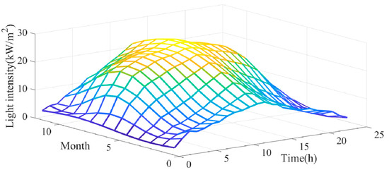
Figure A1.
Curve of light intensity.
References
- Gong, S.Y.; Wei, W.; Xu, Y.F.; Zhai, X.L.; Xu, R.K. Reconfiguration of distribution network for the maximum consumption of distributed generations. Proc. CSU-EPSA 2017, 29, 7–11. [Google Scholar]
- Ding, Y.; Wang, F.; Bin, F.; Zhou, W. Multi-objective distribution network reconfiguration based on game theory. Electr. Power Autom. Equip. 2019, 39, 28–36. [Google Scholar]
- Yang, M.; Zhai, H.F.; Ma, J.Y.; Wei, S.P.; Wang, M.X.; Dong, Q.L. Dynamic reconfiguration of three-phase unbalanced distribution networks considering unbalanced operation constraint of distributed generation. Proc. CSEE 2019, 39, 3486–3499. [Google Scholar]
- Santos, J.D.; Marques, F.; Negrete, L.P.G.; Brigatto, G.A.A.; López-Lezama, J.M.; Muñoz-Galeano, N. A Novel Solution Method for the Distribution Network Reconfiguration Problem Based on a Search Mechanism Enhancement of the Improved Harmony Search Algorithm. Energies 2022, 15, 2083. [Google Scholar] [CrossRef]
- Ullah, K.; Jiang, Q.; Geng, G.; Khan, R.A.; Aslam, S.; Khan, W. Optimization of Demand Response and Power-Sharing in Microgrids for Cost and Power Losses. Energies 2022, 15, 3274. [Google Scholar] [CrossRef]
- Radwan, A.A.; Foda, M.O.; Elsayed, A.H.M.; Mohamed, Y.S. Modeling and reconfiguration of middle Egypt distribution network. In Proceedings of the 2017 Nineteenth International Middle East Power Systems Conference (MEPCON), Cairo, Egypt, 19–21 December 2017; pp. 1258–1264. [Google Scholar]
- Chen, C.; Wang, S.; Liu, B.; An, Y.; Huang, C.; Huang, X.Y. A Fast Network Reconfiguration Method Avoiding Infeasible Solutions for Distribution System. Trans. China Electrotech. Soc. 2015, 30, 34–43. [Google Scholar]
- Gerez, C.; Coelho Marques Costa, E.; Sguarezi Filho, A.J. Distribution Network Reconfiguration Considering Voltage and Current Unbalance Indexes and Variable Demand Solved through a Selective Bio-Inspired Metaheuristic. Energies 2022, 15, 1686. [Google Scholar] [CrossRef]
- Sayed, M.M.; Mahdy, M.Y.; Abdel Aleem, S.H.E.; Youssef, H.K.M.; Boghdady, T.A. Simultaneous Distribution Network Reconfiguration and Optimal Allocation of Renewable-Based Distributed Generators and Shunt Capacitors under Uncertain Conditions. Energies 2022, 15, 2299. [Google Scholar] [CrossRef]
- Zhang, L.Y.; Meng, K.; Liu, S.; Li, Z.Y. Reconstruction of ship power system network fault based on improved two particle swarm algorithm. Power Syst. Prot. Control. 2019, 47, 90–96. [Google Scholar]
- Xie, Y.X.; Liu, T.Q.; Su, X.N. A novel skeleton network reconfiguration method based on distributed PSO algorithm and Hadoop architecture. Power Syst. Technol. 2018, 42, 886–893. [Google Scholar]
- Yang, X.M.; Lv, H.F.; Zhu, H. Reconfiguration of distribution network based on improved artificial fish swarm algorithm. Electr. Meas. Instrum. 2020, 57, 72–78. [Google Scholar]
- Ding, Y.; Wang, F.; Bin, F.; Yan, W.T.; Zhou, W. Fast network reconfiguration considering distributed power supply uncertainty. Proc. CSU-EPSA 2018, 30, 57–63. [Google Scholar]
- Bucciarelli, M.; Paoletti, S.; Vicino, A. Optimal sizing of energy storage systems under uncertain demand and generation. Appl. Energy 2018, 225, 611–621. [Google Scholar] [CrossRef]
- Zhu, Y.Q.; Zhang, L.; Zhang, S.Q.; Wang, T.J. Optimal scheduling strategy for battery ES system based on ordered charge-discharge. Smart Power 2019, 47, 23–29. [Google Scholar]
- Zhao, X.Q.; Qin, L.J.; Duan, H. Distributed ES optimal scheduling of distribution network based on aggregation effect. Power Capacit. React. Power Compens. 2020, 41, 228–234. [Google Scholar]
- Chen, Z.; Liu, Y.; Chen, X.; Zhou, T.; Xing, Q. Charging and discharging dispatching strategy for EV considering characteristics of mobile ES. Autom. Electr. Power Syst. 2020, 44, 77–85. [Google Scholar]
- Li, Y.; Yang, Z.; Li, G.Q.; Mu, Y.F.; Zhao, D.B.; Chen, C.; Shen, B. Optimal scheduling of isolated microgrid with an EV battery swapping station in multi-stakeholder scenarios: A bi-level programming approach via real-time pricing. Appl. Energy 2018, 232, 54–68. [Google Scholar] [CrossRef] [Green Version]
- Li, H.; Li, G.J.; Wang, K.Y. Real-time dispatch strategy for EV based on deep reinforcement learning. Autom. Electr. Power Syst. 2020, 44, 161–167. [Google Scholar]
- Liu, D.; Cao, J.; Liu, M. Joint Optimization of Energy Storage Sharing and Demand Response in Microgrid Considering Multiple Uncertainties. Energies 2022, 15, 3067. [Google Scholar] [CrossRef]
- Alimohammadisagvand, B.; Jokisalo, J.; Kai, S. In The potential of predictive control in minimizing the electricity cost in a heat-pump heated residential house. In Proceedings of the 3rd IBPSA-England Conference BSO 2016, Newcastle, UK, 12–14 September 2016; IBPSA-England, Loughborogh University: Loughborough, UK, 2016. [Google Scholar]
- Alimohammadisagvand, B. Influence of Demand RESPONSE actions on Thermal Comfort and Electricity Cost for Residential Houses. Ph.D. Thesis, Aalto University, Espoo, Finland, 2018. [Google Scholar]
- Liu, Z.F.; Chen, Y.X.; Zhuo, R.Q.; Jia, H.J. Energy storage capacity optimization for autonomy microgrid considering CHP and EV scheduling. Appl. Energy 2018, 210, 1113–1125. [Google Scholar] [CrossRef]
- Baptista, J.E.R.; Rodrigues, A.B.; da Silva, M.D. Probabilistic Analysis of PV Generation Impacts on Voltage Sags in LV Distribution Networks Considering Failure Rates Dependent on Feeder Loading. IEEE Trans. Sustain. Energy 2019, 10, 1342–1350. [Google Scholar] [CrossRef]
- Tong, X.Q.; Ma, Q.; Tang, K.Y.; Liu, H.K.; Li, C. Influence of EV access mode on the static voltage stability margin and accommodated capacity of the distribution network. J. Eng. 2019, 2019, 2658–2662. [Google Scholar] [CrossRef]
- Song, X.T.; Weng, Z.P.; Zhou, J.H.; Xu, W.Y.; Zhao, Y.X. Reliability evaluation and planning of microgrid based on whole time sequence simulation of multi-state uncertainty. High Volt. Eng. 2020, 46, 1508–1517. [Google Scholar]
- Han, Y.; Yang, B.; Byun, H. Optimizing actuators deployment for WSAN using hierarchical intermittent communication particle swarm optimization. IEEE Sens. J. 2021, 21, 847–856. [Google Scholar] [CrossRef]
- Li, Z.W.; Zhao, S.Q.; Liu, J.S. Optimal scheduling of power system based on dependent-chance goal programming. Proc. CSEE 2019, 39, 2803–2816. [Google Scholar]
- Peng, C.H.; Yu, Y.; Sun, H.J. Planning of combined PV-ESS system for distribution network based on source-network-load collaborative optimization. Power Syst. Technol. 2019, 43, 3944–3951. [Google Scholar]
- Weng, X.Y.; Tan, Y.H. Load restoration strategy for unbalanced distribution network considering active power temporal-spatial supporting of mobile energy storage. Power Syst. Technol. 2021, 45, 1463–1470. [Google Scholar]
- Sanaullah, K.; Xia, M.C.; Hussain, M.; Hussain, S.; Tahir, A. Optimal islanding for restoration of power distribution system using Prim′s MST algorithm. CSEE J. Power Energy Syst. 2020, 8, 599–608. [Google Scholar]
- Asrari, A.; Lotfifard, S.; Payam, M.S. Pareto dominance-based multiobjective optimization method for distribution network reconfiguration. IEEE Trans. Smart Grid 2016, 7, 1401–1410. [Google Scholar] [CrossRef]
- Baran, M.E.; Wu, F.F. Network reconfiguration in distribution systems for loss reduction and load balancing. IEEE Trans. Power Deliv. 1989, 4, 1401–1407. [Google Scholar] [CrossRef]
Publisher’s Note: MDPI stays neutral with regard to jurisdictional claims in published maps and institutional affiliations. |
© 2022 by the authors. Licensee MDPI, Basel, Switzerland. This article is an open access article distributed under the terms and conditions of the Creative Commons Attribution (CC BY) license (https://creativecommons.org/licenses/by/4.0/).