Estimation of Unmeasured Room Temperature, Relative Humidity, and CO₂ Concentrations for a Smart Building Using Machine Learning and Exploratory Data Analysis

Abstract

Smart buildings that utilize innovative technologies such as artificial intelligence (AI), the internet of things (IoT), and cloud computing to improve comfort and reduce energy waste are gaining popularity. Smart buildings comprise a range of sensors to measure real-time indoor environment variables essential for the heating, ventilation, and air conditioning (HVAC) system control strategies. For accuracy and smooth operation, current HVAC system control strategies require multiple sensors to capture the indoor environment variables. However, using too many sensors creates an extensive network that is costly and complex to maintain. Our proposed research solves the mentioned problem by implementing a machine-learning algorithm to estimate unmeasured variables utilizing a limited number of sensors. Using a six-month data set collected from a three-story smart building in Japan, several extreme gradient boosting (XGBoost) models were designed and trained to estimate unmeasured room temperature, relative humidity, and CO₂ concentrations. Our models accurately estimated temperature, humidity, and CO₂ concentration under various case studies with an average root mean squared error (RMSE) of 0.3 degrees, 2.6%, and 26.25 ppm, respectively. Obtained results show an accurate estimation of indoor environment measurements that is applicable for optimal HVAC system control in smart buildings with a reduced number of required sensors.

1. Introduction

As civilization advances, indoor environments have become our predominant habitat because we spend much of our time indoors for work and accommodation. Building occupants’ health, well-being, and productivity depend on four aspects of indoor environmental quality (IEQ): thermal comfort, visual comfort, acoustics, and indoor air quality [1,2]. Thermal comfort is the most prevalent factor of the four categories. Arif et al. in [3] showed that good thermal comfort levels inspired occupant productivity in commercial buildings. For example, a slight increase in indoor temperature above ideal decreased occupant cognitive performance [4].

In Tokyo, Japan, the world’s largest metropolitan city, commercial buildings consume about 36% of the total energy usage. The heating, ventilation, and air conditioning (HVAC) systems alone account for approximately 40% of the total building energy consumption worldwide [5,6]. Experts are responsible for regularly monitoring and physically operating the installed HVAC system in traditional buildings. Human errors, such as forgetting to turn off the system on days when no one is in the building, will inevitably result in energy waste when HVAC systems are manually controlled. HVAC control can be automated in today’s smart buildings by adjusting HVAC systems based on user preferences to boost occupant comfort and save energy waste.

Innovative technologies are helping to accelerate the development of smart buildings [7] to ensure that people can live in a more pleasant, intelligent, and energy-efficient environment. A smart building is distinguished from an ordinary building because it can sense its environment using sensors, actuators, smart meters, and the ability to respond intelligently to achieve desired goals [6,8]. Smart buildings incorporate three major components: hardware, software, and a communication network. Hardware includes sensors, actuators, and smart meters. The software components are computer programs that collect and analyze data from sensors and meters and then implement control strategies. Examples of software components include building energy management systems (BEMS) and machine learning algorithms that extract useful information from the raw data. A communication network acts as the nervous system of the building [6,8]. All these components fall into the trending category of Internet of Things (IoT) technology, where multiple devices will interconnect over the internet and store large amounts of data in the cloud. Artificial intelligence (AI) is a data-driven technique that utilizes such data to optimize the HVAC system performance of smart buildings.

Estimating indoor room temperature and relative humidity is essential for optimal HVAC control strategies. Currently, thermal estimation models are implemented using building simulations such as EnergyPlus [9]. Simulations are extensively used during the design stage [10] to predict a building’s thermal and electrical parameters. On the other hand, building simulation models are based on prior knowledge gathered during the design stage and require lengthy and sometimes complex configurations. These models are also impractical for real-world applications as they do not consider real-world indoor environment variables and are not capable of coping with model drift or the change in building operation [11]. Sensor-based real-time indoor environment variables monitoring, on the contrary, is a viable solution to this issue [12,13]. The wireless sensor network (WSN) and IoT techniques based on real-time indoor environment data transcend the limitations of simulation-based approaches. Nonetheless, maintaining a giant sensor and communication network is expensive and complex [10].

Many researchers have extensively studied various data-driven algorithms for forecasting a building’s energy consumption and environmental variables such as temperature, humidity, and CO₂ concentration. Energy wastage is reduced by optimally controlling the HVAC system’s operations, which also improves the thermal comfort of occupants. From the algorithm perspective, machine learning (ML) based techniques that learn historical data trends and thermal behaviors have attracted significant research attention [14]. In [15], researchers compared the accuracy of various building energy consumption forecasting models such as linear regression, ridge regression, K-Nearest Neighbors regressor, Random Forest regressor, gradient Boosting regressor, Extra Trees regressor, MLP regressor, and Artificial Neural Networks (ANNs). Their findings show that ANN models are the best alternative for short-term load forecasting (STLF). Other different case studies mentioned in [16,17] showed that 1D-CNNs outperformed LSTM, shallow ANNs, and SVM models based on root mean squared error (RMSE) evaluation. Ref. [18] went a step further, combining 1D-CNN with LSTM to form a CNN-LSTM hybrid model that outperformed the other ML models in short-term load forecasting.

The article [19] proposed a plug-and-play building thermal model learning framework integrated with any IoT-based BEM system. The proposed framework only relies on data collected from low-cost IoT-based smart thermostats, which are affordable for most building owners. However, plug-and-play devices also create an extensive and complex network that is difficult to maintain. In [20], the authors proposed combining time-series analysis and neural networks to conduct room temperature prediction using the collected temperature data. However, their model was tested using simulated data obtained from EnergyPlus software [9]. Simulation-based models are unreliable when implemented in real-world applications. Chen and Li [21] used a Bayesian Model Fusion technique to estimate the temperature in a smart building. However, they did not include humidity in their study, an essential parameter for occupants’ thermal comfort. Nivine Attoue et al. [22] used outdoor temperature and facade sensor data as input features to their ANN-based model to forecast indoor temperature to optimize the building’s energy devices. Other studies employ artificial neural networks (ANNs) to predict the indoor temperature and other indoor environment variables in smart buildings [17,22,23]. ANN models, in general, give more accurate estimations of non-linear data. However, ANN models usually require plenty of data for training and are time-consuming.

The [24] review article compared 36 different ML algorithms to forecast indoor temperature in a smart building. Researchers tested the models using actual smart building data and compared their accuracy using R-coefficient and RMSE metrics. According to their findings, the ExtraTrees regressor model obtained the best accuracy across all forecasting horizons. Their results showed the power of decision tree-based models in predictive modeling. Xiaoming Ma et al. [25] used historical outdoor temperature and relative humidity data to make predictions of both outdoor temperature and humidity using the extreme gradient boosting (XGBoost) algorithm. Their XGBoost model achieved excellent performance when evaluated using R-squared and RMSE statistical metrics. However, their prediction horizon was only between 1 to 3 h. Unlike other ML predictive algorithms, XGBoost is more generalized to different amounts of data sets, and its performance on the training set and test set is very consistent. Although there are plenty of ML algorithms for indoor environmental variables prediction, the computing time required for most is longer than XGBoost models. Minimal training time is necessary to meet the needs of real-time prediction scenarios.

This paper presents a methodology for accurately estimating unmeasured indoor air temperature, relative humidity, and CO₂ concentration within room areas without sensors for a building in Japan. Consequently, the novelty of our methodology is the design of simple extreme gradient boost (XGBoost) models that can utilize limited data for training and make accurate estimations. The two primary contributions of our methodology are:

• Reduced number of sensors required for optimal indoor environment variable measurements in a commercial building.
• Accurate indoor temperature and relative humidity estimation for HVAC system control to reduce energy waste while improving occupant thermal comfort.

The remainder of this paper is laid out as follows: Section 2 introduces the XGBoost machine learning algorithm and outlines the data analysis techniques. Section 3 shows the estimation results of different case studies. Section 4 discusses the results and their shortcomings. Finally, Section 5 provides some concluding observations and future works.

2. Materials and Methods

2.1. XGBoost Machine Learning Algorithm

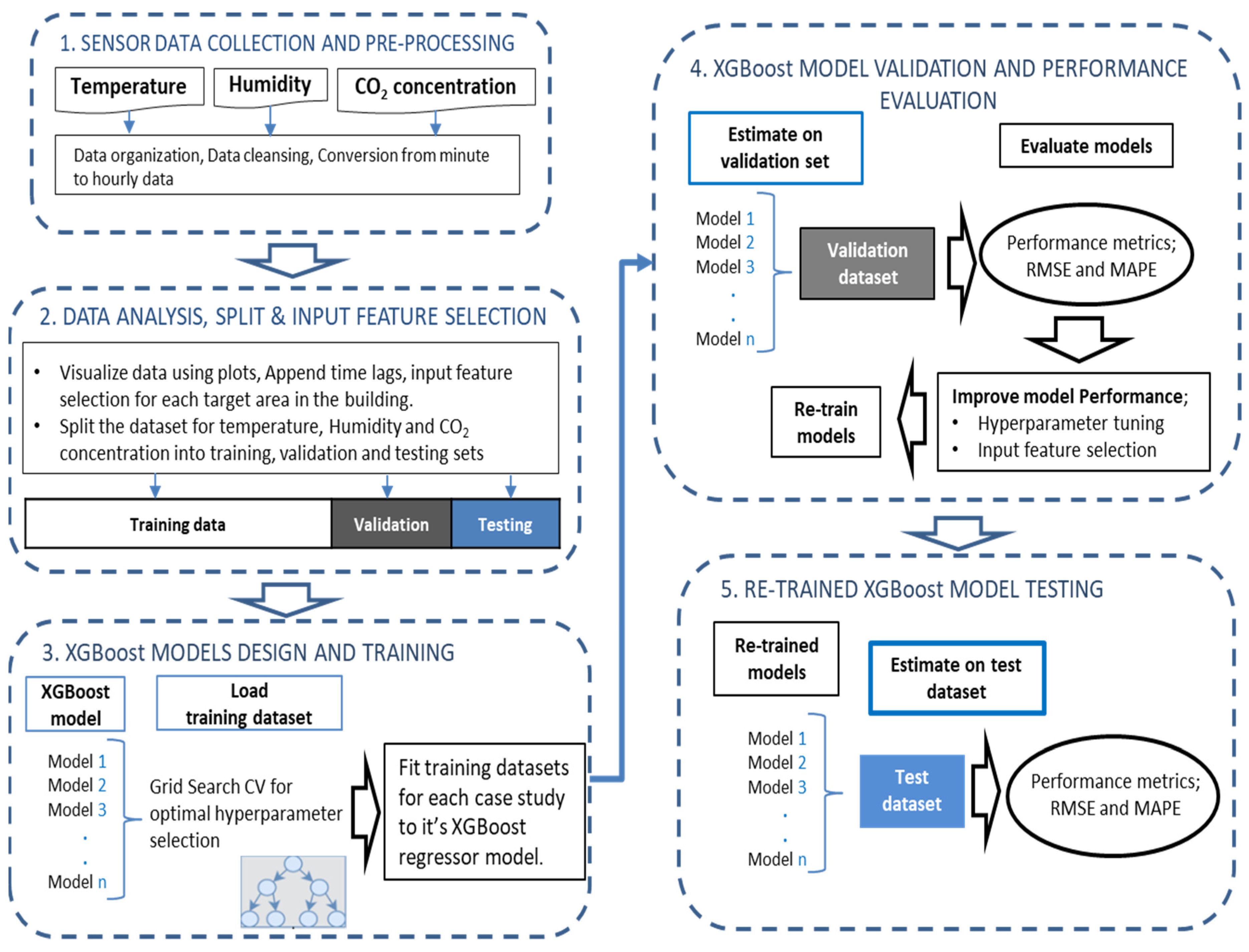
The XGBoost algorithm is a scalable machine learning system for tree boosting. It was first proposed by Chen and Guestrin [26] and has been widely recognized as one of the best algorithms for solving machine learning and data mining challenges [25]. XGBoost provides a parallel tree boosting technique that combines a set of weak learners with a strong learner using additive training steps. The additive learning steps can be described as follows.

Initially, the first tree is fitted to the entire data space, and then a second learner is fitted to the residuals to address the shortcomings of the previous learner. The fitting procedure is repeated several times until the halting conditions are satisfied. The algorithm’s final predictive outcome is derived by summing up the predictions of all learners. Equation (1) illustrates the predictive function at a time step, t.

$${{\displaystyle f}}_i^{(t)}={\displaystyle \sum _{k=1}^t{{\displaystyle f}}_k}\left({{\displaystyle x}}_i\right)={{\displaystyle f}}_i^{(t-1)}+{{\displaystyle f}}_t\left({{\displaystyle x}}_i\right),$$

(1)

where x_i is the input variable, f_t(x_i) is the learner at time step t, f_i^(t) is the prediction at step t, and f_i^(t−1) is the prediction at step t − 1.

XGBoost model implements the following Equation (2) to evaluate the effectiveness of the model from the original function:

$$obj={\displaystyle \sum _{i=1}^{n}l\left({{\displaystyle y}}_i,{{\displaystyle \widehat{y}}}_i\right)}+{\displaystyle \sum _{i=1}^t\Omega \left({{\displaystyle f}}_i\right)},$$

(2)

where l is the loss function, n is the number of observations, ŷ_i is the estimated value, y_i is the actual value, and Ω is the regularization term and defined in Equation (3) as:

$$\Omega \left(f\right)=\gamma T+\frac{1}{2}\lambda {\Vert \omega \Vert }^2,$$

(3)

where ω is the vector of leaf scores, λ is the regularization parameter, and γ represents the minimal loss required for the leaf node to split. The detailed information and computation procedures of the XGBoost algorithm can be found in Chen and Guestrin [26].

2.2. Methodology

In this section, the steps to estimate the temperature, relative humidity, and CO₂ concentrations of an office building used in our case study are described in detail. The building used in our research is a certified zero energy building (ZEB) [27] in Japan. Figure 1 illustrates the methodology process overview.

2.2.1. Data Collection and Pre-Processing

The building used in our research is a 3-story building with a basement and a rooftop. Each floor has a few rooms. Multiple sensor devices are installed in all the rooms to measure one-minute interval building environment parameters, i.e., temperature, relative humidity, CO₂ concentration, and send them to a local server for storage. For our study, a six-month data set was utilized.

The raw data set obtained for our case study was very unstructured. It comprised daily data files of one-minute intervals and contained unnecessary data with a small percentage of missing data. The first step in all machine learning projects is to prepare the data set into the required format for the training algorithm. Therefore, we started by extracting temperature, relative humidity, and CO₂ concentration data from the large data set. Then, we combined all daily data files into one large file. After that, we analyzed different techniques to handle missing data. Missing data points were randomly scattered throughout the whole data set. We tried various interpolation methods and finally employed the spline interpolation method found in the Pandas python library. The data set was then converted into hourly intervals and visualized.

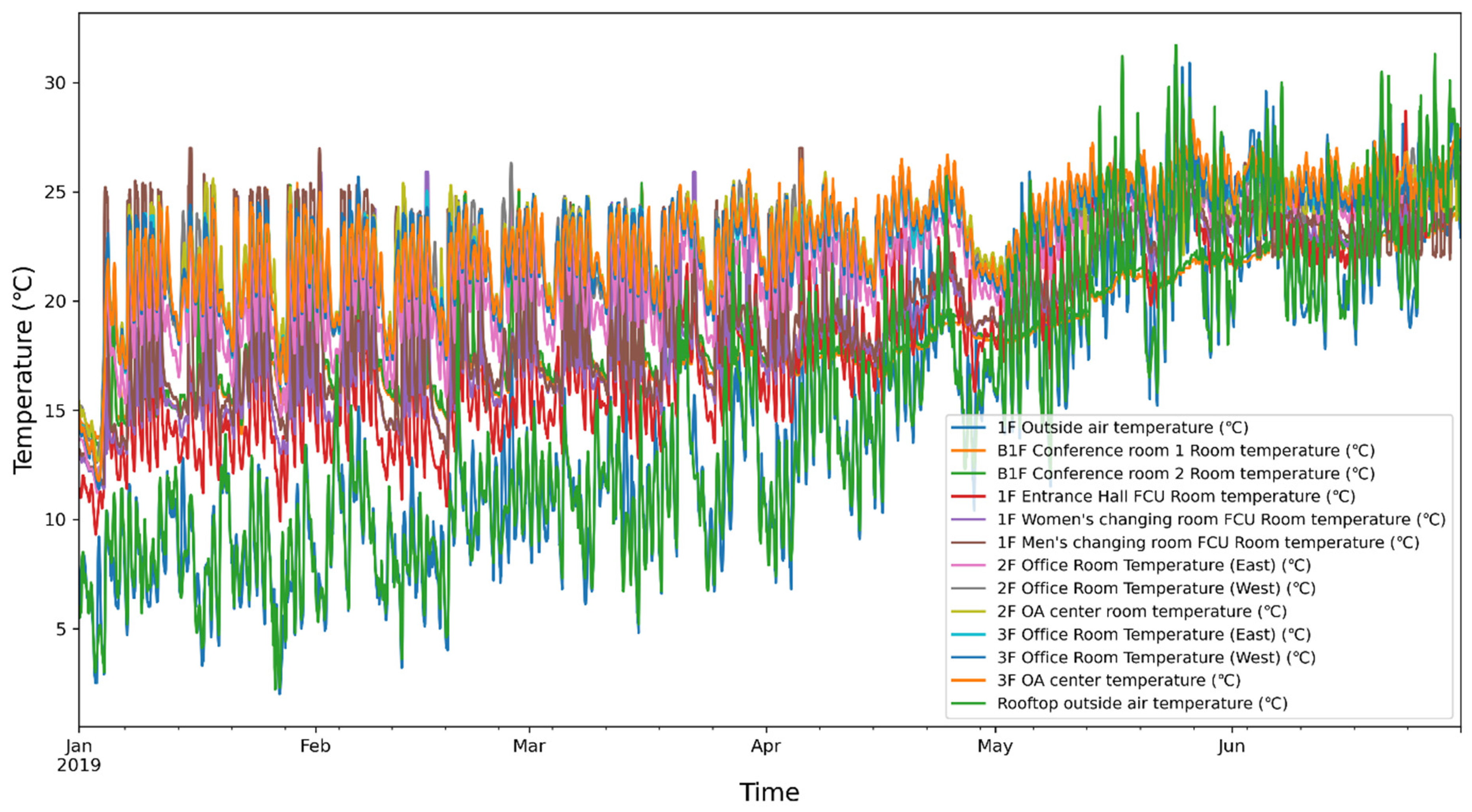
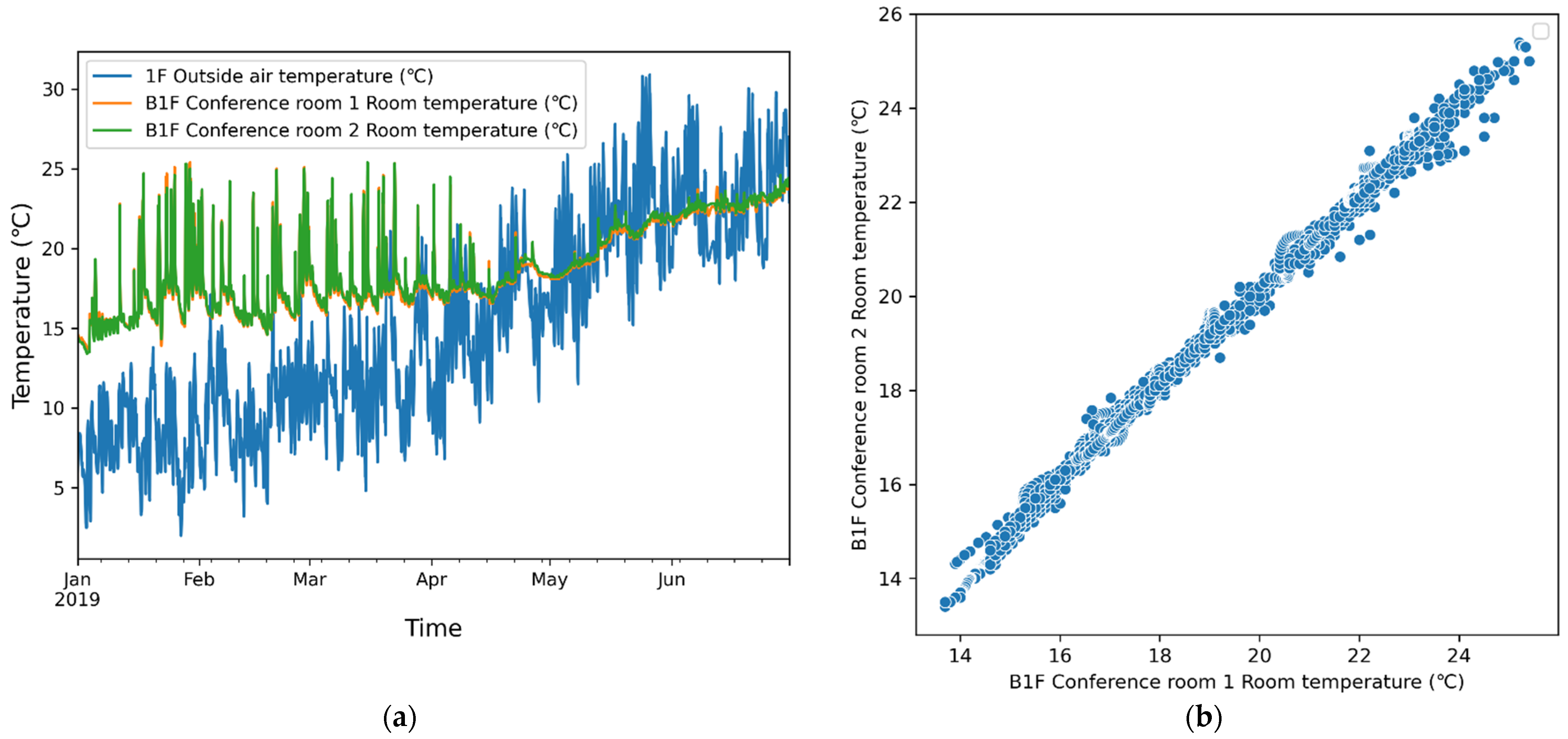
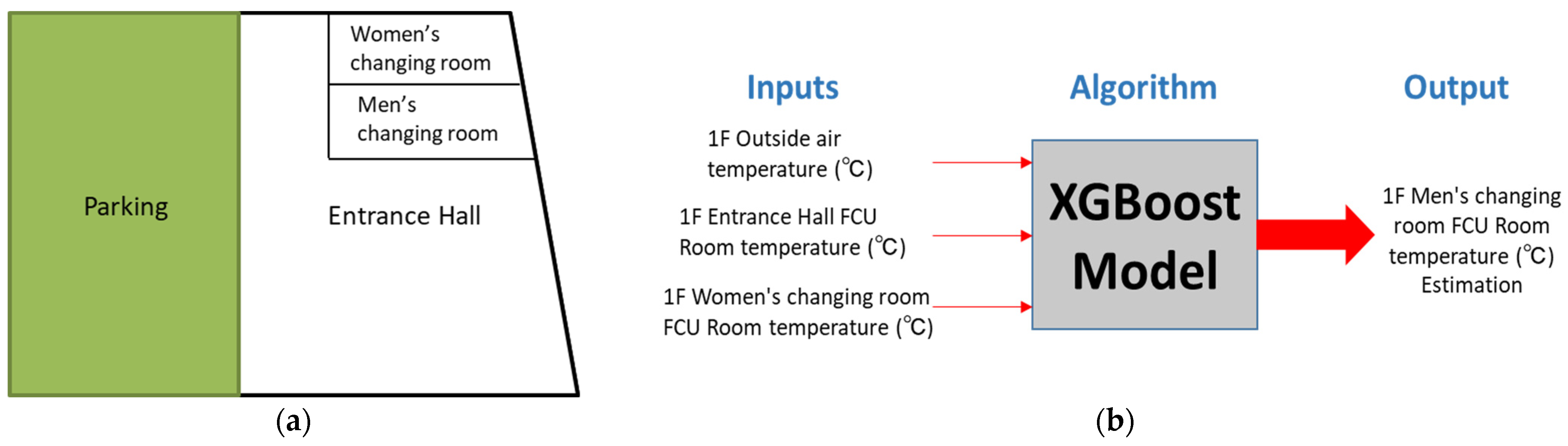
2.2.2. Data Analysis and Input Feature Selection

After preparing and pre-processing the data set, the time series plots were made to visualize indoor room temperature, relative humidity, and CO₂ concentration. Figure 2 depicts cleansed temperature data for all building rooms from January 2019 to June 2019.

The building used in our case study comprises four floors and a rooftop. Each floor has multiple rooms. Each room was equipped with sensors from which we collected the data. In addition to the indoor room sensors, we also collected data from outside the building and on the rooftop. For example, the basement comprises two rooms, i.e., B1F conference room 1 and B1F conference room 2. One of the research objectives is to reduce the number of sensors in a building by estimating indoor environment variables of one room based on data collected from neighboring rooms. Therefore, we looked for the correlation between data from B1F conference room 1, B1F conference room 2, and the outside. Figure 3a is a time series plot for outside air temperature, B1F conference room 1 temperature, and B1F conference room 2 temperature. Figure 3b is a scatter plot of B1F conference room 1 temperature and B1F conference room 2 temperature. Both figures show a high correlation between the data points of both rooms; hence, data from B1F conference room 1 can be used to estimate the temperature in B1F conference room 2 and vice versa.

The first floor consists of three rooms. We collected data from 1F entrance hall, men’s changing room, and women’s changing room. These data were analyzed, and correlations were extracted between each room and the outside data readings. In machine learning, the accuracy of models is dependent on the importance of the selected input features. Therefore, we separated the data set into temperature, humidity, and CO₂ concentration data sets, then carried out input feature engineering.

To begin with, we computed a Pearson correlation matrix between all the variables. It returned values between −1 and 1, where values close to 1 show a high positive correlation, close to zero shows no correlation, and close to −1 show a high negative correlation between the variables. Next, correlation matrices for each floor and outside data variables were computed, and their result guided us in selecting the suitable target rooms (outputs) for indoor environment estimation and the necessary inputs for each case study. For example, on the first floor of the building in Figure 4a, we used outside air temperature, 1F entrance hall room temperature, and 1F women’s changing room temperature as inputs to estimate 1F men’s changing room temperature, as depicted in Figure 4b. The same approach was repeated for relative humidity and CO₂ concentration estimation modeling.

Time series data are sequential; hence, current values correlate with their historical values. Each observation is dependent on its previous value. We, therefore, added hourly time lags of each target output as an input to our estimation models. Selection of optimal time lags [15] for time series forecasting is of crucial importance for accurate results. Figure 5 is a correlation matrix with time lags for the selected optimal input features for the model described in Figure 4.

2.2.3. XGBoost Model Design, Training, Testing, and Evaluation

Our models were designed using the XGBRegressor module found in the XGBoost library. The algorithm was implemented using Python language. Before inputting the data into the models, the data were randomly split into training, validation, and test sets. The XGBRegressor model was fitted with the training set of four months of historical temperature, humidity, and CO₂ concentration data during the training stage. The model has hyperparameters that were initially set to default values. However, the default value will not always give the best accuracy for all cases. Therefore, tuning the hyperparameters for each case is necessary to obtain the best possible estimation accuracy. Our research achieved this by employing the grid search CV [28] technique borrowed from the Scikit learn library [29]. Grid search cross-validation is a tuning technique that uses cross-validation to perform an exhaustive search over specified parameter values of an estimator.

The commonly tunable hyperparameters with their optimal values for each model are described in

Table 1. Hyperparameters for training XGBoost Models.

Hyperparameter	Model 1	Model 2	Model 3	Model 4	Model 5	Model 6	Description
max_depth	4	2	4	3	2	2	Maximum depth of each tree (1–10)
n_estimators	400	50	200	400	400	400	Number of trees in the ensemble
colsample_bytree	1	1	1	1	1	1	Number of features used in each tree
min_child_weight	1	1	1	1	1	1	Minimum sum of weight needed in a child
learning_rate	0.3	0.3	0.3	0.3	0.3	0.3	The learning rate used to weigh each step

.

In Table 1, Models 1 to 6 represent basement conference room 2, men’s changing room, 2nd-floor west room, 2nd-floor OA center room, 3rd-floor east room, and 3rd-floor OA center room temperature estimation.

The data for May 2019 were used for model validation. The purpose of the validation data set is to pretest the models before the final test. Then, based on the performance evaluation of the estimation results on the validation set, the models were retrained using different hyperparameters and inputs until the best performance scores were obtained.

The evaluation of all the designed models was realized by computation of 2 commonly used performance metrics. These are the mean absolute percentage error (MAPE) and the root mean squared error (RMSE) [30] described by Equations (4) and (5):

$$\mathrm{MAPE}=\frac{100}{n}{\displaystyle \sum _{i=1}^n\frac{\left|{{\displaystyle y}}_i-{{\displaystyle \widehat{y}}}_i\right|}{{{\displaystyle y}}_i}},$$

(4)

$$\mathrm{RMSE}=\sqrt{{\displaystyle \sum _{i=1}^n\frac{{\left({{\displaystyle y}}_i-{{\displaystyle \widehat{y}}}_i\right)}^2}{n}}},$$

(5)

where ŷ_i is the estimated value, y_i is the actual value, and n is the number of samples.

3. Results

This section is dedicated to the experimental results obtained after testing all models. After model hyperparameter tuning and the selection of optimal input features, indoor room temperature, relative humidity, and CO₂ concentration were estimated and evaluated using RMSE and MAPE performance metrics.

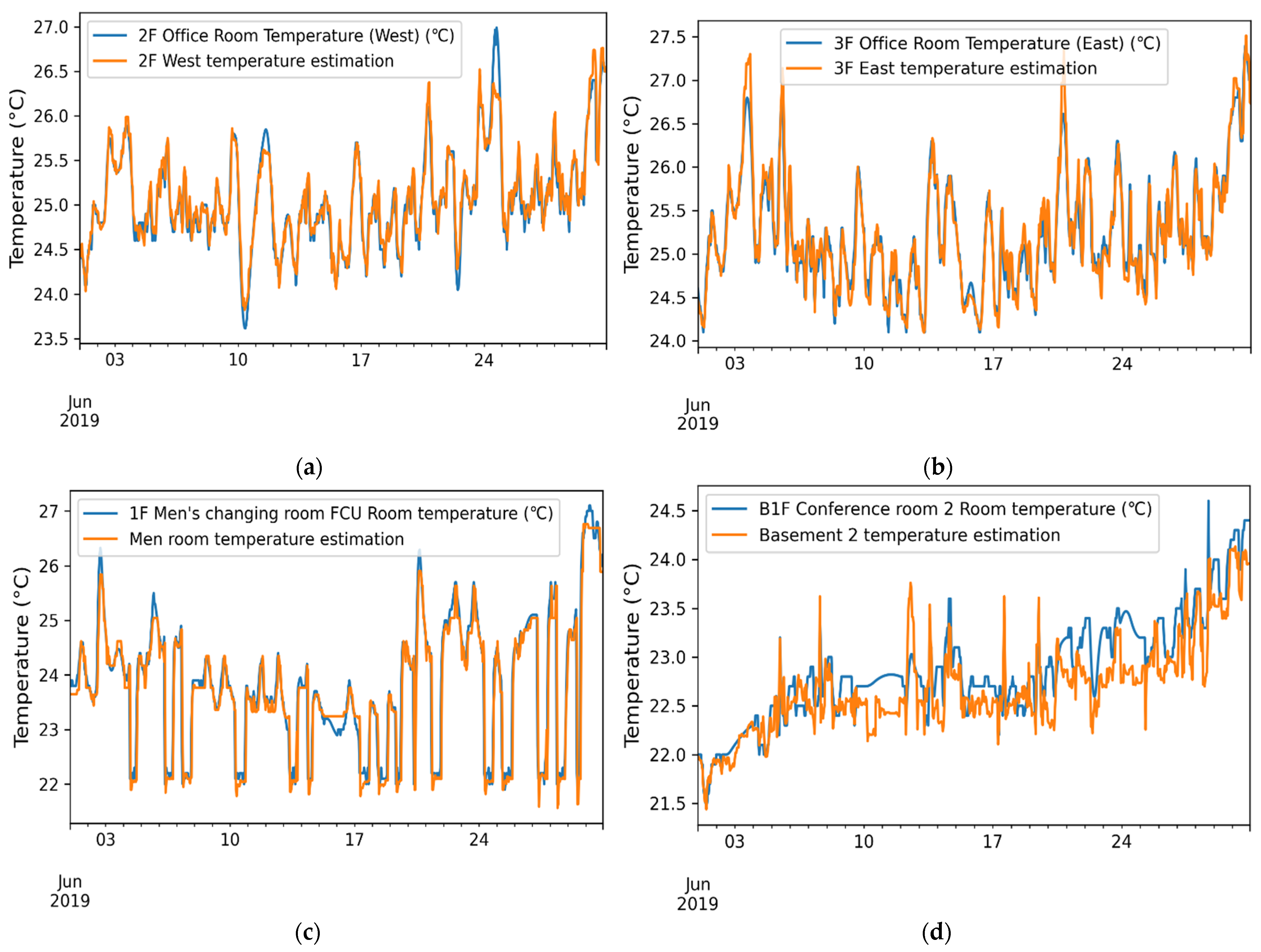
3.1. Indoor Temperature Estimation Results

The indoor temperature of each selected room has a slightly different characteristic trend which is reliant on the number of occupants, air-conditioning operation, and availability of other heat-generating equipment such as servers and computers. After an exploratory data analysis described in the previous chapter, six rooms were selected as targets for temperature estimation. Estimation of the temperature of each room was explicitly modeled for that room, that is, a specific model and a specific set of input features.

After training, the models were tested on the test data set of June 2019. The line plots of actual temperature data and the estimated room temperature for four of the six selected rooms are shown in Figure 6. They reveal a good fit and stable estimation for a medium-term horizon of one month.

The performance evaluation results of each selected room are summarized in

Table 2. Performance metrics for selected rooms on the validation and test temperature sets.

Selected Building Rooms	Validation RMSE	Test RMSE	Test MAPE
B1F Conference room 2	0.2101	0.4632	1.0656
1F Men’s changing room	0.3741	0.4340	0.9707
2F Office Room (West)	0.2906	0.1467	0.4204
2F OA center room	0.3312	0.3134	0.8392
3F Office Room (East)	0.4236	0.1736	0.5060
3F OA center	0.3155	0.2436	0.6374

using RMSE and MAPE evaluation metrics. The models were first tested on the validation set of May 2019, retrained, and then tested on June 2019 data. The RMSE score represents the error in degrees Celsius, and MAPE depicts the estimation error as a percentage. The maximum error of about 0.46 degrees and an average RMSE value of about 0.3 degrees represent the models’ temperature estimation accuracy.

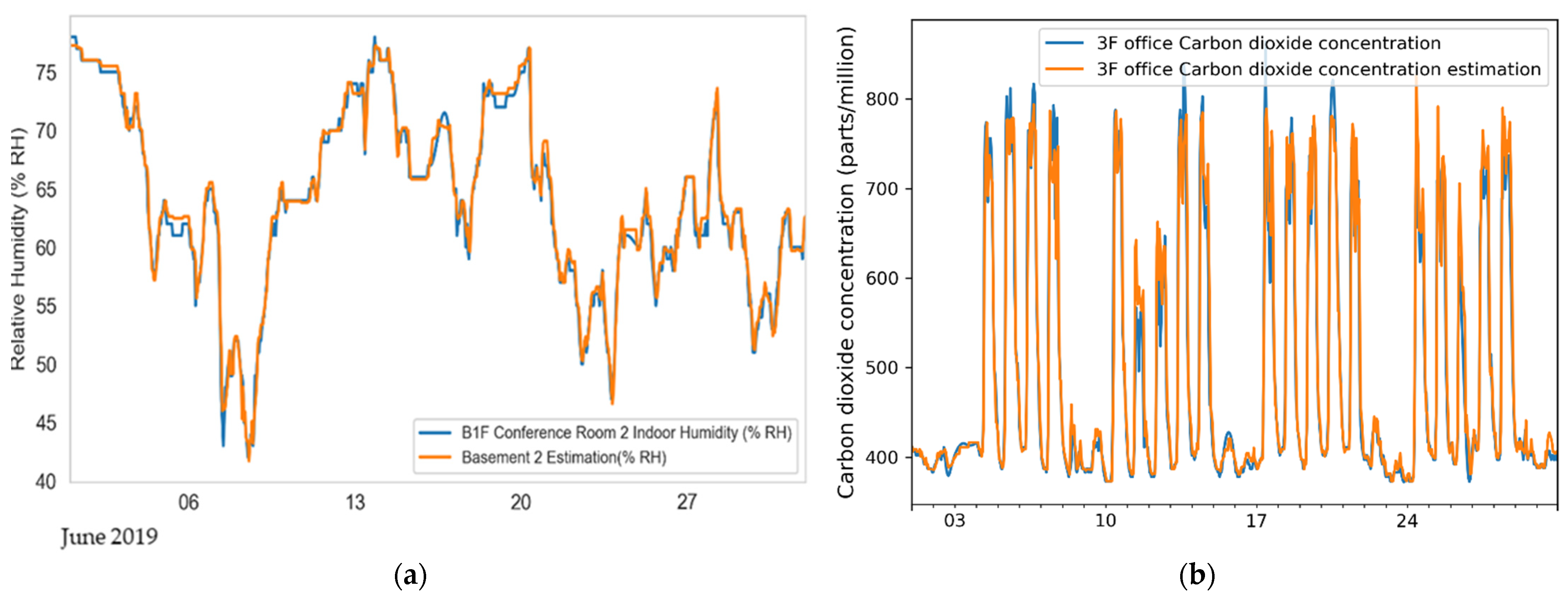
3.2. Relative Humidity and CO₂ Concentration Estimation Results

Like the temperature, each room’s data trend characteristics of relative humidity and CO₂ concentration are slightly different; hence, each case requires a specific XGBoost model and a specific set of input features. We, therefore, employed exploratory data analysis techniques on the relative humidity and CO₂ concentration data sets. Optimal hyperparameters for each model were carefully obtained, and essential input features were extracted from the data.

Due to the space limitation, we cannot provide the test results for all the selected rooms for relative humidity and CO₂ concentration estimation. However, Figure 7 compares the basement conference room 2 relative humidity and third-floor office CO₂ concentration estimations with the actual test set. Again, the estimations are a good fit, depicting the excellent accuracy of the designed models.

The performance evaluation results of each selected room are summarized in

Table 3. Performance evaluation metrics results for relative humidity and CO₂ concentration.

Selected Building Rooms	Relative Humidity RMSE	Relative Humidity MAPE	CO2 Conc. RMSE	CO2 Conc. MAPE
B1F Conference Room 2	1.0992	1.1175	19.2314	1.5552
Cool Pit	2.9769	2.2044	N/A	N/A
2F Office Room (East)	2.9958	2.5130	N/A	N/A
2F OA center room	3.1536	2.696	N/A	N/A
3F Office Room (West)	2.9958	2.4096	33.3331	3.3610
3F OA center	2.7648	2.4707	N/A	N/A

. Six cases were estimated for relative humidity, and only two cases were estimated for CO₂ concentration estimation because we only had data from four CO₂ concentration sensors installed in the two basement rooms, the second and third floors of the building.

On average, the relative humidity estimation was accurate to about 2.6% RH, and the CO₂ concentration was accurate to an average of 26.25 ppm in terms of RMSE evaluation metrics scores. This represents a good fit and shows the power of XGBoost algorithms in the precise estimation of indoor environment variables necessary for occupant well-being and control policies for the smooth operation of heating and cooling systems in a building.

4. Discussion

To begin with, we had 13 data points for temperature, 11 data points for relative humidity, and 5 data points for CO₂ concentration. For the temperature estimation, we utilized data from seven data points to estimate the temperature for six rooms, as shown in Table 2. This implies that the proposed temperature XGBoost model reduced the number of temperature sensors from 13 to 7, representing a reduction of about 50%. The relative humidity estimation XGBoost models utilized five data points to estimate relative humidity for six rooms (Table 3), while The CO₂ concentration estimation XGBoost models used three data points to estimate CO₂ concentration for two floors, as shown in Table 3.

For temperature estimation, the obtained average RMSE score of 0.3 is very accurate and acceptable based on the conventional evaluation metrics for regression algorithms. The humidity estimation models obtained an average RMSE metric score of 2.6, and the CO₂ concentration models obtained an average RMSE metric score of 26.25. These errors appear prominent in value because they are dependent on a different range of scales for the estimated environment variables. However, the MAPE evaluation metric, which depicts the estimation errors as a percentage, indicated an error of 2.2342% and 2.4581% for relative humidity and CO₂ concentration estimation, respectively, representing a good estimation.

However, the accuracy of machine learning models for estimating indoor environment variables relies on the quality of data used for their training. As a limitation, the data collected did not include any indoor activities. Indoor activities, such as meetings, using energy-intensive devices, and opening and closing doors and windows can substantially influence a room’s environmental variables. Future research should consider integrating indoor activities in their modeling to improve the estimation accuracy. Furthermore, using more data for model training could ultimately improve the accuracy.

In our future works, we will also design a reinforcement learning agent to automatically control the HVAC systems in a smart building [31]. Temperature and relative humidity estimation models will be used to generate the simulated environment from which the agent will learn for optimal automatic control of HVAC systems with a goal of occupant comfortability and energy efficiency.

5. Conclusions

This paper proposed using simple XGBoost machine learning algorithms to estimate a commercial building’s indoor room temperature, relative humidity, and CO₂ concentration. Following the discussion of results, the adopted models accurately estimated both RMSE and MAPE metric scores. Modeling and accurately estimating indoor environmental variables in buildings is an essential task for reducing the overall energy consumption of the building and improving occupant comfortability.

The proposed XGBoost models are applicable to commercial and residential buildings as a practical solution because they do not require a big data set for training. Additionally, the models can be deployed on basic and affordable computer hardware. The proposed models also reduce the necessity for multiple sensors that create expensive and complicated networks that are difficult to maintain.

References

1. Frontczak, M.; Wargocki, P. Literature survey on how different factors influence human comfort in indoor environments. Build. Environ. 2011, 46, 922–937. [Google Scholar] [CrossRef]
2. Heinzerling, D.; Schiavon, S.; Webster, T.; Arens, E. Indoor environmental quality assessment models: A literature review and a proposed weighting and classification scheme. Build. Environ. 2013, 70, 210–222. [Google Scholar] [CrossRef] [Green Version]
3. Al Horr, Y.; Arif, M.; Kaushik, A.; Mazroei, A.; Katafygiotou, M.; Elsarrag, E. Occupant productivity and office indoor environment quality: A review of the literature. Build. Environ. 2016, 105, 369–389. [Google Scholar] [CrossRef] [Green Version]
4. Provins, K.A. Environmental heat, body temperature, and behavior: An hypothesis. Aust. J. Psychol. 2007, 18, 118–129. [Google Scholar] [CrossRef]
5. Rezaie, B.; Rosen, M.A. Department of Environment and Energy HVAC Energy Breakdown. HVAC Hess 2013, 93, 36–37. [Google Scholar]
6. Manic, M.; Amarasinghe, K.; Rodriguez-Andina, J.J.; Rieger, C. Intelligent Buildings of the Future: Cyber aware, Deep Learning Powered, and Human Interacting. IEEE Ind. Electron. Mag. 2016, 10, 32–49. [Google Scholar] [CrossRef]
7. Weng, T.; Agarwal, Y. From buildings to smart buildings-sensing and actuation to improve energy efficiency. IEEE Des. Test Comput. 2012, 29, 36–44. [Google Scholar] [CrossRef]
8. Batov, E.I. The distinctive features of “smart” buildings. Procedia Eng. 2015, 111, 103–107. [Google Scholar] [CrossRef] [Green Version]
9. Crawley, D.B.; Lawrie, L.K.; Winkelmann, F.C.; Buhl, W.F.; Huang, Y.J.; Pedersen, C.O.; Strand, R.K.; Liesen, R.J.; Fisher, D.E.; Witte, M.J.; et al. EnergyPlus: Creating a new-generation building energy simulation program. Energy Build. 2001, 33, 319–331. [Google Scholar] [CrossRef]
10. Chen, X.; Li, X. Virtual temperature measurement for smart buildings via Bayesian model fusion. Proc.-IEEE Int. Symp. Circuits Syst. 2016, 2016, 950–953. [Google Scholar] [CrossRef]
11. Ghahramani, A.; Galicia, P.; Lehrer, D.; Varghese, Z.; Wang, Z.; Pandit, Y. Artificial Intelligence for Efficient Thermal Comfort Systems: Requirements, Current Applications, and Future Directions. Front. Built Environ. 2020, 6, 109807. [Google Scholar] [CrossRef]
12. Dong, B.; Prakash, V.; Feng, F.; O’Neill, Z. A review of a smart building sensing system for better indoor environment control. Energy Build. 2019, 199, 29–46. [Google Scholar] [CrossRef]
13. Han, Z.; Gao, R.X.; Fan, Z. Occupancy and indoor environment quality sensing for smart buildings. In Proceedings of the 2012 IEEE International Instrumentation and Measurement Technology Conference Proceedings, Graz, Austria, 13–16 May 2012; pp. 1–6. [Google Scholar]
14. Wei, Y.; Zhang, X.; Shi, Y.; Xia, L.; Pan, S.; Wu, J.; Han, M.; Zhao, X. A review of data-driven approaches for prediction and classification of building energy consumption. Renew. Sustain. Energy Rev. 2018, 82, 1027–1047. [Google Scholar] [CrossRef]
15. Bouktif, S.; Fiaz, A.; Ouni, A.; Serhani, M.A. Optimal deep learning LSTM model for electric load forecasting using feature selection and genetic algorithm: Comparison with machine learning approaches. Energies 2018, 11, 1636. [Google Scholar] [CrossRef] [Green Version]
16. Amarasinghe, K.; Marino, D.L.; Manic, M. Deep neural networks for energy load forecasting. In Proceedings of the 2017 IEEE 26th International Symposium on Industrial Electronics (ISIE), Edinburgh, UK, 19–21 June 2017; pp. 1483–1488. [Google Scholar] [CrossRef]
17. Kaligambe, A.; Fujita, G. Short-Term Load Forecasting for Commercial Buildings Using 1D Convolutional Neural Networks. In Proceedings of the 2020 IEEE PES/IAS PowerAfrica, Nairobi, Kenya, 25–28 August 2020. [Google Scholar] [CrossRef]
18. He, K.; Zhang, X.; Ren, S.; Sun, J. Delving deep into rectifiers: Surpassing human-level performance on imagenet classification. In Proceedings of the IEEE International Conference on Computer Vision, Santiago, Chile, 7–13 December 2015; pp. 1026–1034. [Google Scholar] [CrossRef] [Green Version]
19. Zhang, X.; Pipattanasomporn, M.; Chen, T.; Rahman, S. An IoT-Based Thermal Model Learning Framework for Smart Buildings. IEEE Internet Things J. 2020, 7, 518–527. [Google Scholar] [CrossRef]
20. Aliberti, A.; Ugliotti, F.M.; Bottaccioli, L.; Cirrincione, G.; Osello, A.; MacIi, E.; Patti, E.; Acquaviva, A. Indoor Air-Temperature Forecast for Energy-Efficient Management in Smart Buildings. In Proceedings of the 2018 IEEE International Conference on Environment and Electrical Engineering and 2018 IEEE Industrial and Commercial Power Systems Europe (EEEIC/I&CPS Europe), Palermo, Italy, 12–15 June 2018. [Google Scholar] [CrossRef]
21. Chen, X.; Li, X.; Tan, S.X.D. Overview of cyber-physical temperature estimation in smart buildings: From modeling to measurements. In Proceedings of the 2016 IEEE Conference on Computer Communications Workshops (INFOCOM WKSHPS), San Francisco, CA, USA, 10–14 April 2016; pp. 251–256. [Google Scholar] [CrossRef]
22. Attoue, N.; Shahrour, I.; Younes, R. Smart building: Use of the artificial neural network approach for indoor temperature forecasting. Energies 2018, 11, 395. [Google Scholar] [CrossRef] [Green Version]
23. Soleimani-Mohseni, M.; Thomas, B.; Fahlén, P. Estimation of operative temperature in buildings using artificial neural networks. Energy Build. 2006, 38, 635–640. [Google Scholar] [CrossRef]
24. Alawadi, S.; Mera, D.; Fernández-Delgado, M.; Alkhabbas, F.; Olsson, C.M.; Davidsson, P. A comparison of machine learning algorithms for forecasting indoor temperature in smart buildings. Energy Syst. 2020, 1–17. [Google Scholar] [CrossRef] [Green Version]
25. Ma, X.; Fang, C.; Ji, J. Prediction of outdoor air temperature and humidity using Xgboost. IOP Conf. Ser. Earth Environ. Sci. 2020, 427, 012013. [Google Scholar] [CrossRef]
26. Chen, T.; Guestrin, C. XGBoost: A scalable tree boosting system. In Proceedings of the ACM SIGKDD International Conference on Knowledge Discovery and Data Mining, Seattle, WA, USA, 14–18 August 2016; Association for Computing Machinery: New York, NY, USA, 2016; Volume 13–17, pp. 785–794. [Google Scholar]
27. Enefice Kyushu|U.S. Green Building Council. Available online: https://www.usgbc.org/projects/enefice-kyushu (accessed on 8 January 2021).
28. Tuning the Hyper-Parameters of an Estimator—Scikit-Learn 0.24.1 Documentation. Available online: https://scikit-learn.org/stable/modules/grid_search.html#grid-search (accessed on 26 January 2021).
29. Scikit-Learn: Machine Learning in Python—Scikit-Learn 0.24.0 Documentation. Available online: https://scikit-learn.org/stable/ (accessed on 14 January 2021).
30. Yildiz, B.; Bilbao, J.I.; Sproul, A.B. A review and analysis of regression and machine learning models on commercial building electricity load forecasting. Renew. Sustain. Energy Rev. 2017, 73, 1104–1122. [Google Scholar] [CrossRef]
31. Gao, G.; Li, J.; Wen, Y. DeepComfort: Energy-Efficient Thermal Comfort Control in Buildings Via Reinforcement Learning. IEEE Internet Things J. 2020, 7, 8472–8484. [Google Scholar] [CrossRef]
Figure 1. Methodology process overview.
Energies 15 04213 g001
Figure 2. Recorded temperature data for the building.
Energies 15 04213 g002
Figure 3. (a) Time series plot for outside air temperature, B1F conference room 1 temperature, and B1F conference room 2 temperature; (b) scatter plot of B1F conference room 1 temperature and B1F conference room 2 temperature.
Energies 15 04213 g003
Figure 4. (a) 1st floor (1F) schematic; (b) estimation approach for 1st floor of the building.
Energies 15 04213 g004
Figure 5. Correlation matrix with time lags for the selected optimal input features.
Energies 15 04213 g005
Figure 6. (a) Plot of actual 2F office room temperature and its estimation for June 2019; (b) plot of actual 3F office room temperature and its estimation for June 2019; (c) plot of actual 1f Men’s changing room temperature and its estimation for June 2019; (d) plot of actual B1F conference room 2 temperature, and its estimation for June 2019.
Energies 15 04213 g006
Figure 7. (a) Plot of actual B1F conference room 2 relative humidity and its estimation for June 2019; (b) plot of actual 3F office room CO2 concentration and its estimation for June 2019.
Energies 15 04213 g007