Optimisation of Buyer and Seller Preferences for Peer-to-Peer Energy Trading in a Microgrid

Abstract

In this paper, an optimisation approach to prioritise buyers and sellers in a peer-to-peer (P2P) energy trading market based on distances from the aggregator has been developed. The proposed approach assigns higher preferences to buyers/sellers with a smaller distance, as this will allow lower losses in the power transmission. Under this approach, the sellers and buyers operate in a decentralised manner to optimise the preference coefficients along with the energy sold/purchased to achieve certain profits/savings. The proposed approach is implemented using a real-life dataset, and the impacts of different parameters, such as seasonal variations in renewable generation, distances and profit thresholds for sellers, have been investigated. The results show that the proposed approach allows buyers and sellers to purchase/sell more energy from the P2P trading market (2.4 times increase when maximum energy sold is considered) in comparison to the case when all participants are equally preferred. It has been observed that, with increasing distances, sellers are assigned a smaller preference coefficient, which results in sellers being willing to sell a higher amount of energy so that they can achieve the same profit threshold.

1. Introduction

The energy demand across the world has been increasing exponentially over the past decade. There has been a widespread growth of small-scale distributed energy generation, which utilises the energy derived from renewable resources to support low-carbon electricity production techniques and schemes initiated by governments [1]. This encompasses rooftop solar systems, behind-the-meter generation, residential energy storage systems and electric vehicle applications [2]. Residential solar energy generation can be used not only to meet the growing electricity demand, but also to integrate cleaner energy into the grid. To promote such local energy generation projects, many countries are offering incentives for microgrids, a miniature version of the utility grid with local generation and demand. In addition, a feed-in-tariff (FIT) scheme has been introduced so that consumers with rooftop solar panels in a microgrid can sell their excess energy back to the utility grid, thereby becoming proactive consumers, also called prosumers [3]. However, the decline in the FIT rate has slowed down the pace of solar panel uptakes and caused a lack of motivation for participation as a prosumer. This has instigated next generation techniques, called peer-to-peer (P2P) energy trading, where the prosumers/consumers can buy or sell energy based on their needs and priorities.

In P2P energy trading, prosumers actively participate in an energy market and directly exchange energy with their peers to maintain a supply and demand balance [4,5]. P2P network architecture is divided into two layers, a virtual layer and a physical layer. The virtual layer is a secure platform through which an information exchange is processed and the proper matching of buying or selling orders via the appropriate market mechanism is performed. Financial transactions are also initiated after the successful matching of orders [6]. The physical layer is the traditional distributed grid system or separate microgrid in conjunction with the main grid system that facilitates the flow of electricity between the peers once the financial settlement is finalised [6]. The advantages of incorporating P2P energy trading include improving the power system’s reliability and lowering the investments and operational costs of the grid, as well as significantly reducing the peak demand with minimised storage requirements. However, overly decentralised energy trading without any coordination and control can compromise the electricity network’s operation. Proper market paradigms, information exchange and pricing mechanisms can ensure that the energy exchange between peers is performed within the technical limits of the grid system and with maximum efficiency.

It is important to note that participation in the P2P trading market is often influenced by the user’s behaviour and choices, and different customer segments can be profiled accordingly to identify their market potentials. From this perspective, research has investigated business models and user preferences for P2P trading. For example, the authors of [7] investigated optimal business models considering user beliefs, attitudes and behavioural controls and evaluated the resulting cost savings for a case study in Germany. On the other hand, for a real P2P trading platform in Switzerland, the authors of [8] studied user interaction and participation in the P2P market through surveys and interviews. They identified two customer segments related to preferences on pricing, which include preferences for fixed pricing set by the regulatory body and automated pricing set by the market. The authors in [9] studied the consumer engagement framework for P2P trading and investigated how this framework motivates consumers to become prosumers and increases energy awareness. Note that this paper studies the design of preferences based on distances only, and thus the consideration of human parameters is outside the scope of this paper.

1.1. Related Works

The various technical paradigms and clearing mechanisms of the P2P energy trading market have been studied with the aims of limiting the energy flow within the technical constraints of the grid and maximising the trading parameters of the prosumers. As mentioned in [6], there are primarily four types of technical approach for designing a P2P energy trading strategy. They are game theory, auction theory, blockchain and constrained optimisation. Game theory is a mathematical approach of strategic decision making among participants, where the action of one player depends on and affects other players in the market. There are non-cooperative games, which involve attaining a stable state called Nash equilibrium, where deviating from their actions from this point unilaterally cannot be any better paid off [10]. On the other hand, cooperative games unite all participants in achieving a stable and optimal solution that is mutually beneficial for all the peers involved in the trading market. Examples of such game theory approaches are the Stackelberg game [11], the coalition formation game [12], the canonical coalition game and Nash games [6]. Double auction theory for P2P energy trading is explained in [13], where potential buyers submit their bids to an auctioneer who is simultaneously responsible for providing information about the electricity prices to potential sellers. The auctioneer will arrange the bids in decreasing order and the reservation prices from sellers in increasing order to generate supply and demand curves with intersection points. The intersection points establish the auction price for corresponding buyers and sellers who then engage in the P2P energy exchange. A clearing policy is usually defined for the allocation of resources and payment activation between the peers [10].

Auction-based pricing strategy using the Recursive Least Square (RLS) method is explained in [2], where each buyer or seller provides an estimated clearing price based on the amount of energy they have to buy/sell according to the energy demand and clearing price at previous points in time. For a buyer, the clearing price is the bidding price, whereas, for a seller, the clearing price is the offer price. All clearing prices are arranged in ascending order, and the absolute difference between the buyer’s bidding price and the clearing price is calculated for obtaining the customer’s priorities. The smaller the difference, the higher the priority. Finally, the selling or buying price is calculated for the present time, and the process is recursive in nature. Another pricing strategy is the mid -market rate (MMR) [2], where the energy exchange price is mid-way between the electricity buying price and selling price. Here, the buying and selling price depends on the amount of generation and demand within a neighbourhood. On the other hand, with the bill sharing (BS) method [2], a single electricity bill of a community is shared among the households within that community according to the reading in the utility meter connected at a point between the community microgrid and main grid. Every customer will pay the same unit price for their energy consumption and receive payment at another unit price for their energy generation.

Enabling technologies for P2P energy trading include blockchain-based platforms for a secure and transparent trading through a data structure that can be shared between the involved parties of the market. Information, including the time period for the energy exchange, the amount of energy to be exchanged, the price of the energy to be exchanged and the transaction details about the seller and buyer, can be securely stored and examined using this data structure [14]. This avoids the need for a centralised authority and reduces the reliance on a third-party agent. Blockchain-based platforms such as Elecbay, Smart contract, consortium blockchain, Ethereum and Hyperledger follow this decentralised process, which can be utilised for P2P trading. The impact of information sharing uncertainties and an effective communication scheme to mitigate such uncertainties in a blockchain based system for P2P energy trading applications were investigated in [15]. A smart energy hub that utilises cooperative-relay-aided communication between prosumers and distributed control-architecture for P2P energy trading was proposed in [16]. Another key aspect of P2P energy trading is the optimisation tools, which are required to optimise how much energy needs to be sold/purchased in the P2P market. In particular, constrained optimisation techniques maximise or minimise soft and hard constraints imposed by the power system and market, according to the required optimisation levels for P2P trading [6]. Popular methods of constrained optimisation technique include linear programming (LP), mixed-integer linear programming (MILP), the alternating direction method of multipliers (ADMM) and nonlinear programming (NLP) [6,17].

Bilateral contract networks are used to create forward and real-time scalable markets, as explained in [18], involving energy contracts among three types of agents—prosumers, suppliers and generators. Characteristics such as the upstream–downstream balance of energy and forward market uncertainty are considered in this method. Upstream contracts need to be selected from the lowest to highest prices by the market participants, whereas downstream contracts need to be selected from the highest to lowest prices. The utility-maximising preferences for forward and real-time are presented, which facilitates a stable network of contracts with information regarding energy trades and prices. The optimisation of preferences in [18] poses a distributed price adjustment process that requires decision making and communication between local agents or peers only when there is no central entity. A direct energy-trading method among multiple microgrids is presented in [19] as a Generalised Nash Bargaining (GNB) problem. This technique considers the operational constraints of a distribution network and maximises social welfare by distributing the revenue among the microgrids accordingly. The non-convexity of the problem is managed with two phases. In the first phase, an optimal power flow is solved to determine the energy exchange volume using ADMM. The second phase determines the market clearing price and mutual payments of the microgrids [19].

A decentralised market-clearing mechanism is analysed in [20], which considers the privacy of prosumers, power losses in the transmission line and the cost of utilising a third-party-owned network. The welfare of prosumers is maximised in this method by taking into account the grid usage of each customer, the distance of each energy transaction and the supply–demand balance in the market. A non-convex equality constraint is converted to a convex problem through the Lagrangian relaxation [21], so that it can be solved in a decentralised manner through sub-problems. The power transfer distance from one node to another node in the network is calculated using the Power Transfer Distribution Factor (PTDF). The optimisation problem for the method in [20] is formulated as the difference between the utility of the power demanded and the total money paid, including the energy transaction fee and the network utilisation fee. A modified path optimisation approach is presented in [22], which applies the Physarum Polycephalum algorithm in an energy network for optimising the parameters during P2P energy trading. The variables under consideration are the capacity constraint, the energy flow between producer and consumer, the link cost on the distribution link, the pressure on the links, and the energy density between nodes. This technique can ensure the selection of the optimised path as well as avoiding the usage of congested energy paths as the energy flow and cost of the energy in each link are continuously iterated in every cycle. Another market-clearing mechanism using the knapsack approximation algorithm is presented in [23], which is utilised for trades between one seller and multiple buyers.

A Network Permission structure is explained in [10], where bilateral transactions are estimated using three sensitivity coefficients—the voltage sensitivity coefficient, PTDF and loss sensitivity factors. When a transaction starts, the energy flow and the external or internal costs and losses are estimated with the aforementioned three factors to check whether energy trading is performed within the voltage limits and network capacity. Only those transactions that obey the constraints are initiated in this mechanism. Risk–cost allocation is completed in [24] for the payment transacted by community members, where the Jain index is used as a fairness metric for all cost allocations. Risk-hedging mechanisms in the form of financial contracts are introduced to prevent second-stage losses of agents and to restore fairness in the trading market. In [21], a peer-to-peer automated bilateral negotiation strategy for the energy contract settlement between prosumers is analysed. This technique considers heterogeneous prosumer preferences to make a contract that specifies the volume of energy exchange and the return time of exchanged energy. The negotiating prosumers navigate through a common negotiation domain comprising of potential energy contracts and evaluate those contracts against a utility function. Automated negotiation is an effective strategy for P2P energy trading, as the peers gradually understand their compatibility with other participants in obtaining energy contracts closer to Nash solutions. Moreover, the technique does not require central coordination and a market operator, which is an advantage.

Optimal P2P energy trading needs to take into account the distances between different participants in the market, as a longer distance can add line losses and reduce the effectiveness of local trading. It has been pointed out in the existing literature that the benefits of peer-to-peer energy trading are often outweighed by the network constraints caused by power losses [25,26]. These losses serve as functions of distance [27], and thus users need to be prioritised based on the distance parameters [28]. In this regard, the existing research has considered an electrical distance-driven decentralised double-auction mechanism, which computes a preference list for different buyers/sellers through the distribution system operator [25]. However, this approach does not consider the different weights for participants with different distances, and the preferences are computed centrally. Similarly, the authors in [28] consider priorities based on generation, price or geographical distance, but the pairing between sellers/buyers is coordinated by the central aggregator. The approach in [10] takes into account consumer preferences in terms of user satisfaction to develop the optimisation problem. However, these preferences have not been used to weight the amount of energy sold and purchased. A priority-based optimisation problem for P2P energy trading was considered in [29], but it considers the different energy purchase levels as the priority thresholds and does not account for the distances between sellers/buyers. The authors in [27] considered a system loss-minimisation approach based on non-linear distance optimisation. On the other hand, the authors in [26] incorporate the network topology in the game theoretic model to minimise network losses while maximising profits. However, these papers did not consider the prioritisation of prosumers with smaller distances. A comparison of the proposed approach against related works is illustrated in

Table 1. Comparison of related works against the proposed approach.

Related Works	Mathematical Optimisation	Decentralised Approach	Distance Based Prioritisation	Weighting with Coefficients
[2]	✓	×	×	×
[6]	✓	✓	×	×
[10]	✓	✓	×	×
[11]	×	✓	×	×
[12]	✓	✓	×	×
[13]	✓	×	×	×
[14]	×	✓	×	×
[15]	×	✓	×	×
[16]	×	✓	×	×
[17]	✓	✓	×	×
[30]	×	✓	×	×
[19]	✓	✓	×	×
[25]	✓	✓	✓	×
[28]	✓	✓	✓	×
[29]	✓	×	×	×
Proposed framework	✓	✓	✓	✓

. This shows that, to the best of our knowledge, there has not been any research that weighs the energy sold/purchased with the preference coefficients optimised by sellers/buyers in a decentralised manner based on distance.

1.2. Contributions and Paper Organisation

Though existing research has studied the impact of distances on the power losses in a P2P trading network and prioritising buyers/sellers based on distances, a holistic approach to optimise the energy selling/purchasing decisions while scaling down the energy sales/purchases from participants with larger distances has not been investigated yet. Since users with larger distances can experience more power losses, selling/purchasing more energy to/from these users can result in non-profitable and non-optimal solutions. As a result, it is important that buyers/sellers assign a scaling factor to reduce their energy trading with users at larger distances. Thus, the optimum preference coefficients to scale up/down the energy sale/purchase quantities along with designing the energy sale/purchase decisions need to be optimised jointly to ensure a more efficient P2P trading mechanism.

In this paper, we aim to address the aforementioned research gap through the following contributions:

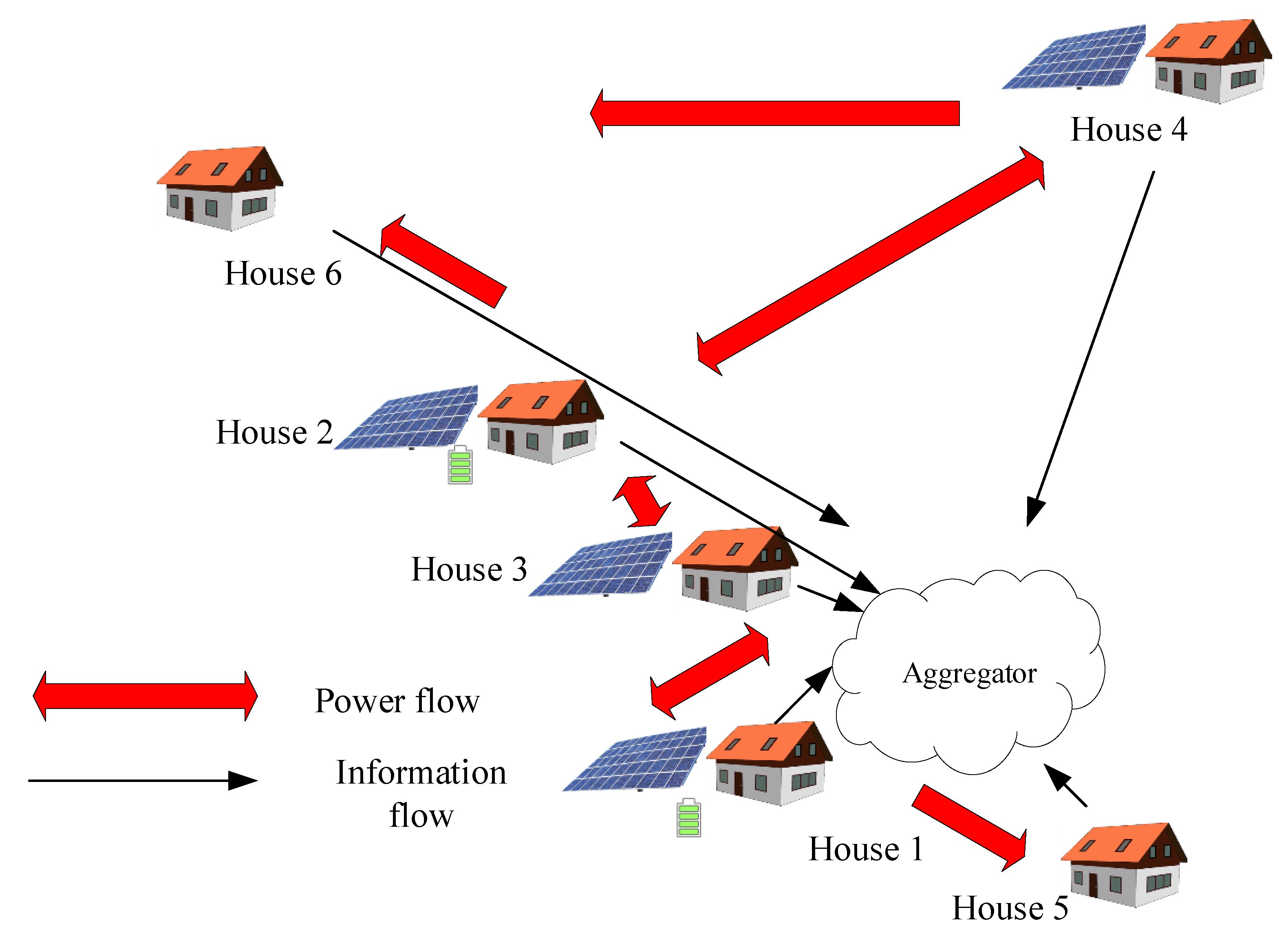
• An optimisation approach for P2P energy trading is developed to account for the preferences of buyers and sellers based on the distances of the participants from the aggregator. The proposed approach offers a decentralised solution to prioritise buyers and sellers, while considering the fact that buyers/sellers with smaller distances will cause fewer losses in the transmission, leading to the higher effectiveness of the P2P trading mechanism.
• The optimisation approach allows individual sellers to optimise the preference coefficients for each buyer in the first stage. In the second stage, each buyer optimises the preference coefficients for each seller based on the energy to be sold and the price asked by that seller. The preference coefficients are utilised as weights of the energy to be sold/purchased by sellers/buyers.
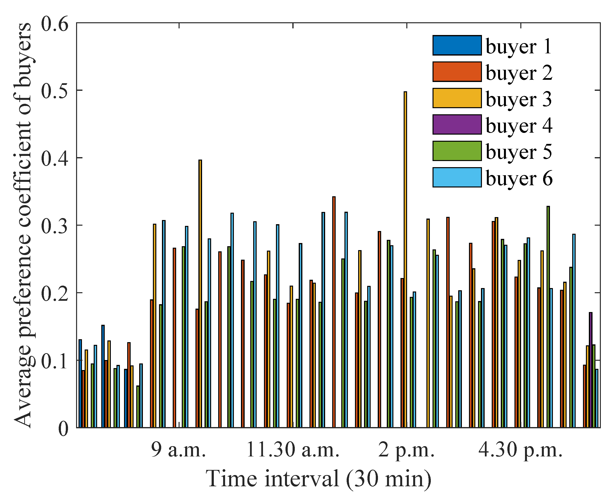
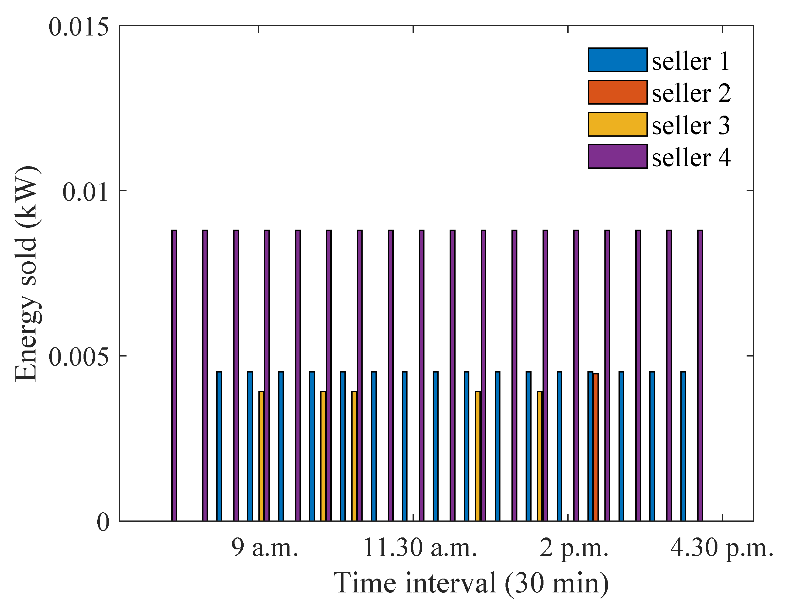
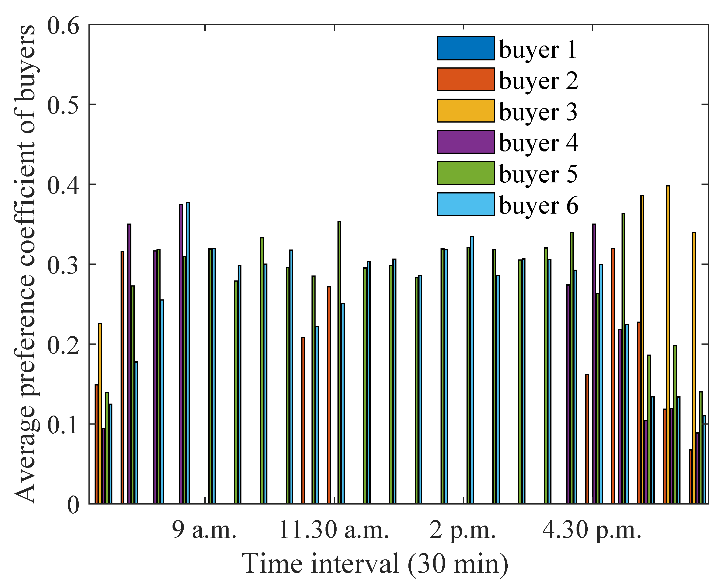
• The proposed approach is evaluated for a real-life energy generation and demand dataset under different scenarios and parameter variations. It can be observed that, when sellers/buyers have a larger distance from the aggregator, they are assigned a smaller preference coefficient.

The rest of the paper is organised in the following manner. Section 2 outlines the approach implemented for the preference coefficient optimisation of the sellers and buyers along with the energy sold and purchased. Section 3 demonstrates the impact of different parameters on the optimisation outcomes by using a real-life dataset. Section 4 elaborates the key findings of this study and their technical and social implications. Finally, Section 5 concludes the paper.

2. Optimisation of Preference Coefficients of Buyers and Sellers

In this section, we outline the optimisation approach for designing the preference coefficients of buyers and sellers in the P2P market while considering distances. We consider a residential microgrid that has houses incorporated with solar panels and/or storage. In addition, we have some more houses which do not have either solar panels or storage, and they participate in the P2P market only as buyers.

As the first step, the daily demand/generation data of all the houses in the P2P market are extracted and forwarded to the aggregator embedded with an energy management system. Based on the excess energy present and electricity deficit, the peers are categorised as sellers and buyers. For houses with a higher distance from the aggregator, power loss in the transmission line is expected to increase as well. This may incur additional charges to the participants in the P2P market, since they must cater for the lost energy in the network links. Therefore, in the proposed approach, sellers with smaller distance from the aggregator will be prioritised by the buyer, and sellers will prefer buyers who are nearest to the aggregator.

Once the aggregator identifies the sellers and buyers, the energy deficit information related to each buyer is forwarded to the sellers. The sellers then optimise the preference coefficients for each buyer and how much energy is to be sold to each buyer so that the sellers can achieve the desired profit threshold. The profit threshold is the minimum profit that the seller wants to achieve in a certain time interval by selling energy to the P2P market. Note that the price for energy trading is set by the seller at a value between the utility rate and the feed-in tariff. This is to ensure that P2P trading allows savings/earnings for both buyers and sellers in comparison to the case when they sale/purchase energy to/from the utility. After that, the sellers forward the bids (prices and energy to be sold) to the buyers through the aggregator. Then, the buyers optimise how much energy they want to purchase from each seller and the preference coefficients for each seller in such a way that the buyers can maintain the desired savings threshold. The savings threshold is the savings in electricity cost that the buyer aims to achieve when purchasing energy from the P2P market. The savings in the electricity cost would be the difference between the cost when the entire energy deficit is met from the utility and the cost when the optimum amount of energy is purchased from the P2P market. Finally, the buyers send the bids (energy to be purchased) to the sellers through the aggregator. Any surplus/deficit energy that could not be balanced in the P2P market will be sold to or purchased from the utility grid.

The optimisation approach considers two different stages. In the first stage, the sellers optimise the preference coefficients for individual buyers. Then in the second stage, the buyers optimise the preference coefficients for all available sellers. Note that the optimisation process takes place at the individual sellers/buyers in a decentralised manner without any intervention from the aggregator. The optimisation approach is illustrated in Figure 1. The optimisation problem associated with the two stages is described in the following subsections. The notations in the following subsections have been elaborated in the nomenclature in the Appendix and have not been repeated here for brevity. The Appendix also lists the acronyms used in this paper.

2.1. Optimisation at the Seller Side

The optimisation problem at the jth seller at a certain time interval can be formulated as:

$$\underset{V_{j,i},X_{j,i}}{min}\sum _i{V}_{j,i}{X}_{j,i}{P}_j,$$

(1)

subject to:

$$\begin{array}{cc}\hfill & X_{j,i}\ge 0\hfill \end{array}$$

(2)

$$\begin{array}{cc}\hfill & 0\le V_{j,i}\le 1\hfill \end{array}$$

(3)

$$\begin{array}{cc}\hfill & V_{j,1}>V_{j,2}>...>V_{j,B}\mathrm{for}{d}_1<d_2<...<d_B\hfill \end{array}$$

(4)

$$\begin{array}{cc}\hfill & \sum _i{X}_{j,i}\le G_j-D_j+u(S_j^{\prime }-S_j)\hfill \end{array}$$

(5)

$$\begin{array}{cc}\hfill & V_{j,i}{X}_{j,i}\le D_i-G_i\hfill \end{array}$$

(6)

$$\begin{array}{cc}\hfill & P_j\sum _i{V}_{j,i}{X}_{j,i}\ge P_{\mathrm{thresh}}\hfill \end{array}$$

(7)

$$\begin{array}{cc}\hfill & 0\le S_j\le S_{\max }.\hfill \end{array}$$

(8)

The objective function in (1) aims to minimise the energy cost of the total energy sold by the seller to each buyer in the market by optimising the preference coefficient from the jth seller to the ith buyer and the energy sold by the jth seller to the ith buyer. The constraint in (2) ensures that the energy sold is a non-negative value. The trading process will only initiate if the amount of energy to be sold is a non-negative value. The purpose of Equation (3) is to limit the priority coefficient values between one and zero. The buyer with the least distance from the aggregator will be preferred most by the seller. Hence, the priority coefficient of the highest proximity buyer will be the largest, and the priority coefficient of the farthest buyer will be the lowest as constrained by (4). The sellers must meet their demands through their own solar generation and stored energy before selling energy to prospective buyers. Hence, (5) ensures that only the excess energy is sold to the buyers. Moreover, the excess energy sold by a seller should not be more than the energy deficit at any buyer involved in P2P trading, as represented in (6). Equation (7) is a constraint developed to take into account the profit of the energy trading process from sellers’ perspective. The total cost of the energy sold by the seller to all buyers must be higher than the set profit threshold. The storage requirements of a seller with energy storage is satisfied using (8). The excess energy of the seller is stored up to the maximum storage capacity and cannot be discharged beyond the minimum stored energy level.

The aforementioned optimisation problem can be expressed as a non-convex quadratic programming problem and solved with standard solution techniques, such as branch and bound method for non-convex problems in the YALMIP package [31]. The solver utilises linear programming relaxations and convex envelope approximations for implementing the branch and bound method for non-convex problems. The solution approach is based on deploying a lower solver that solves the lower-bounding relaxation problems and an upper solver that computes upper bounds using nonlinear solvers [31]. In this paper, linear programming is chosen as the lower solver, and fmincon (a gradient based optimisation solver for nonlinear continuous functions) is chosen as the upper solver.

Once the optimum energy sold and the preference coefficients are computed by each seller for each buyer and communicated, the second stage of the optimisation approach initiates. The next subsection outlines the optimisation problem on the buyer side.

2.2. Optimisation on the Buyer Side

The optimisation problem on the buyer side can be formulated as:

$$\underset{Y_{i,j},U_{i,j}}{min}\sum _j{P}_j{U}_{i,j}{Y}_{i,j}$$

(9)

subject to:

$$\begin{array}{cc}\hfill & Y_{i,j}\ge 0\hfill \end{array}$$

(10)

$$\begin{array}{cc}\hfill & 0\le U_{i,j}\le 1\hfill \end{array}$$

(11)

$$\begin{array}{cc}\hfill & U_{i,1}>U_{i,2}>...>U_{i,S}\mathrm{for}{d}_1<d_2<...<d_S\hfill \end{array}$$

(12)

$$\begin{array}{cc}\hfill & U_{i,j}{Y}_{i,j}\le X_{j,i}\hfill \end{array}$$

(13)

$$\begin{array}{cc}\hfill & \sum _j{Y}_{i,j}\le D_i-G_i\hfill \end{array}$$

(14)

$$\begin{array}{cc}\hfill & (D_i-G_i)P_u-\sum _j{P}_j{U}_{i,j}{Y}_{i,j}\ge P_{\mathrm{savings}}.\hfill \end{array}$$

(15)

Here, the objective function in (9) is formulated to minimise the energy cost of the total energy purchased by the ith buyer from each seller in the market, by optimising preference coefficient from the ith buyer to all sellers and the energy purchased by the ith buyer from all sellers in a certain time interval. The constraint in (10) ensures that the energy purchased by the ith buyer from the jth seller is a non-negative value. Equation (11) limits the preference coefficient values between zero and one. The highest proximity seller will have the highest preference on the buyer side, as the transmission losses will be significantly less for smaller distances between the seller and the aggregator. Hence, the preference coefficient of the nearest seller will be the largest, and the preference coefficient of the farthest seller will be the smallest, as established in (12). The constraint in (13) ensures that the energy purchased by the ith buyer from the preferred seller is limited by the amount of energy bid by the seller to the ith buyer. Moreover, the total energy purchased by the buyer from all the sellers in the P2P market should not be higher than their actual energy deficit, as represented in (14). Equation (15) is a constraint developed to check for the savings of the energy trading process from buyers’ perspective. The difference between the cost of buyer’s deficit energy purchased at the utility rate and the cost of energy purchased from all the sellers in the P2P market at an energy trading price must be higher than the set savings threshold.

Similar to the seller-side optimisation problem, the optimisation problem on the buyer side is expressed as a non-convex quadratic programming problem and solved using the modified branch and bound method for non-convex problems. Once the optimum preference coefficients and energy to be purchased are computed, the information is forwarded to the sellers through the aggregator. Based on this information, the aggregator settles the P2P market between the sellers and the buyers.

3. Simulation Results

In this section, we consider a case study based on the Ausgrid Solar Electricity dataset [32]. Our case study evaluates the optimum preference coefficients of the sellers and buyers to minimise the energy cost in the P2P energy market comprised of six households whose electricity generation and demand data are obtained from the Ausgrid dataset. Among these houses, houses 1 and 2 are connected with both solar panels and batteries. Houses 3 and 4 are connected with solar panels only. On the other hand, houses 5 and 6 are connected to neither solar panels nor batteries. The solar panel capacities for houses 1, 2, 3 and 4 are $3.78$ kW, $1.62$ kW, 1 kW and 1 kW, respectively. The storage capacities for houses 1 and 2 are 3 kWh and $1.5$ kWh, respectively. Note that the Ausgrid dataset was chosen to utilise real-life generation and demand data in the case study, and other similar datasets can also be used.

The utility rate and the feed-in tariff are considered as $0.3$ AUD/kWh and $0.1$ AUD/kWh, respectively. The energy trading prices are defined as uniformly distributed random variables between the feed-in tariff and the utility rate. The reasoning behind this assumption is that it motivates buyers to purchase at a rate lower than the utility rate and sellers to sell at a rate higher than the feed-in tariff, thus encouraging P2P trading among the participants. The profit and savings thresholds are assumed to be $0.003$ AUD and $0.001$ AUD, respectively. These thresholds can be set to different values as well. However, these thresholds need to be in such a range that the sellers/buyers can achieve them with their given excess generation/energy deficit. The normalised distances of the houses from the aggregator are $0.1$, $0.4$, $0.3$, 1, $0.2$ and $0.8$, respectively. Note that these distances are normalised by the maximum distance between the individual houses and the aggregator. These distances are chosen as representative examples and can be set to any other values between 0 and 1 to repeat this analysis. Figure 2 shows how the different houses are located in the P2P trading network for the case study.

The energy sold/purchased in P2P trading is often impacted by seasonal parameters, given that a higher solar generation can lead to a higher energy excess. Moreover, the profit threshold serves as a critical factor for sellers, as it determines how much energy the seller will sell to achieve at least this threshold. In addition, it is important to assess whether the proposed approach can optimise energy sale/purchase values under different distance parameter settings. To ensure that the aforementioned factors are considered in the evaluation process of the proposed approach, we consider four different scenarios in this case study and compute the energy sold/purchased by different participants, as well as the preference coefficients of different buyers/sellers. These scenarios include: (i) an evaluation of the proposed approach for winter data, (ii) the impact of generation changes during summer, (iii) the impact of the distances between houses and the aggregator and (iv) the impact of the profit threshold. The demand and generation data were collected from 1 July 2012 for all scenarios unless otherwise specified.

The proposed approach is evaluated based on the energy sale and purchase values for the aforementioned scenarios, and the results are compared to identify which simulation parameters increase/decrease these quantities. Note that a loss factor is assumed for each participant in the case study, which is inversely proportional to distance. Then, this loss factor is multiplied by the energy excess/deficit values so that smaller energy amounts are available to sell/consume at the seller/buyer. An accurate estimation of the network losses will require a power flow study, which is beyond the scope of this work.

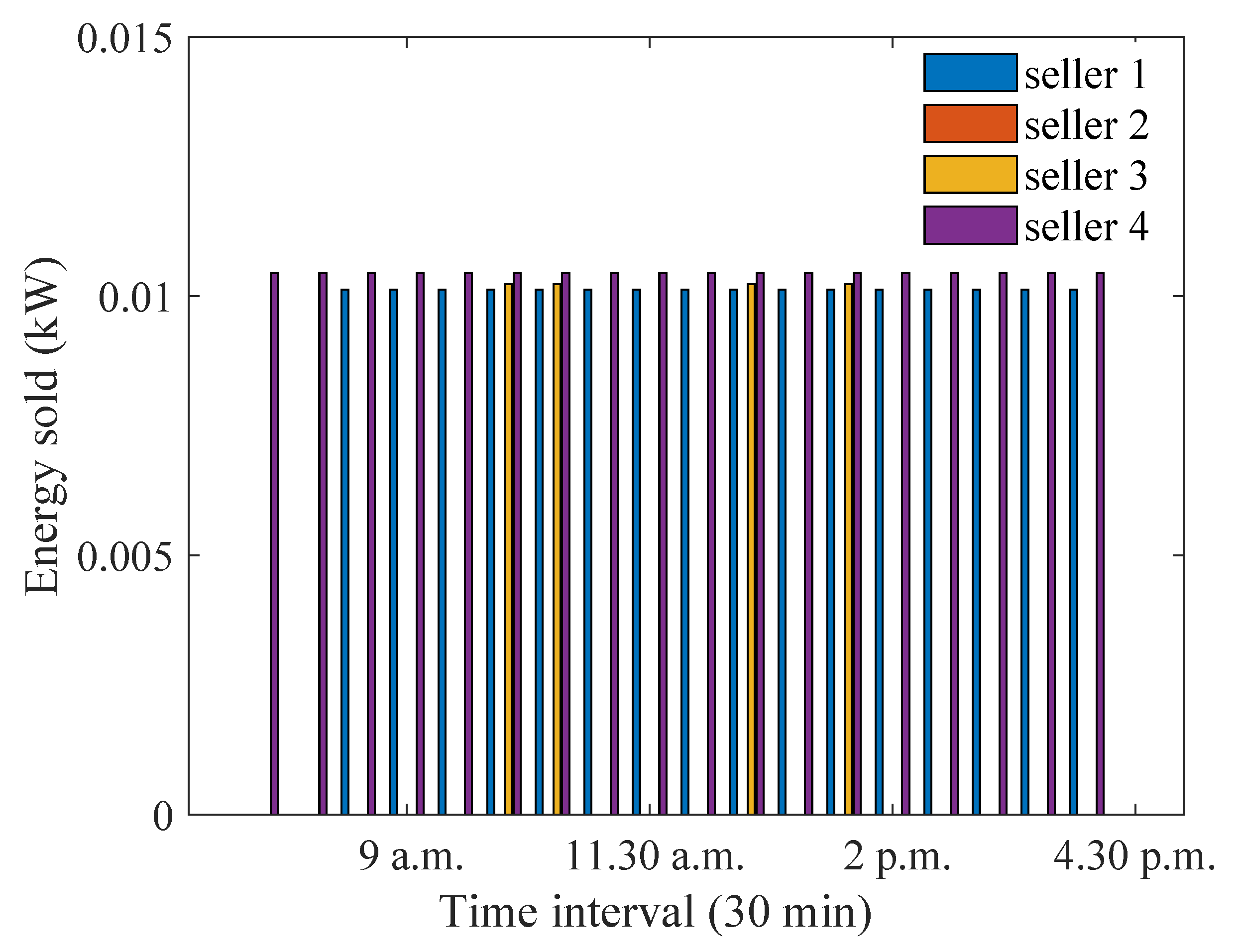
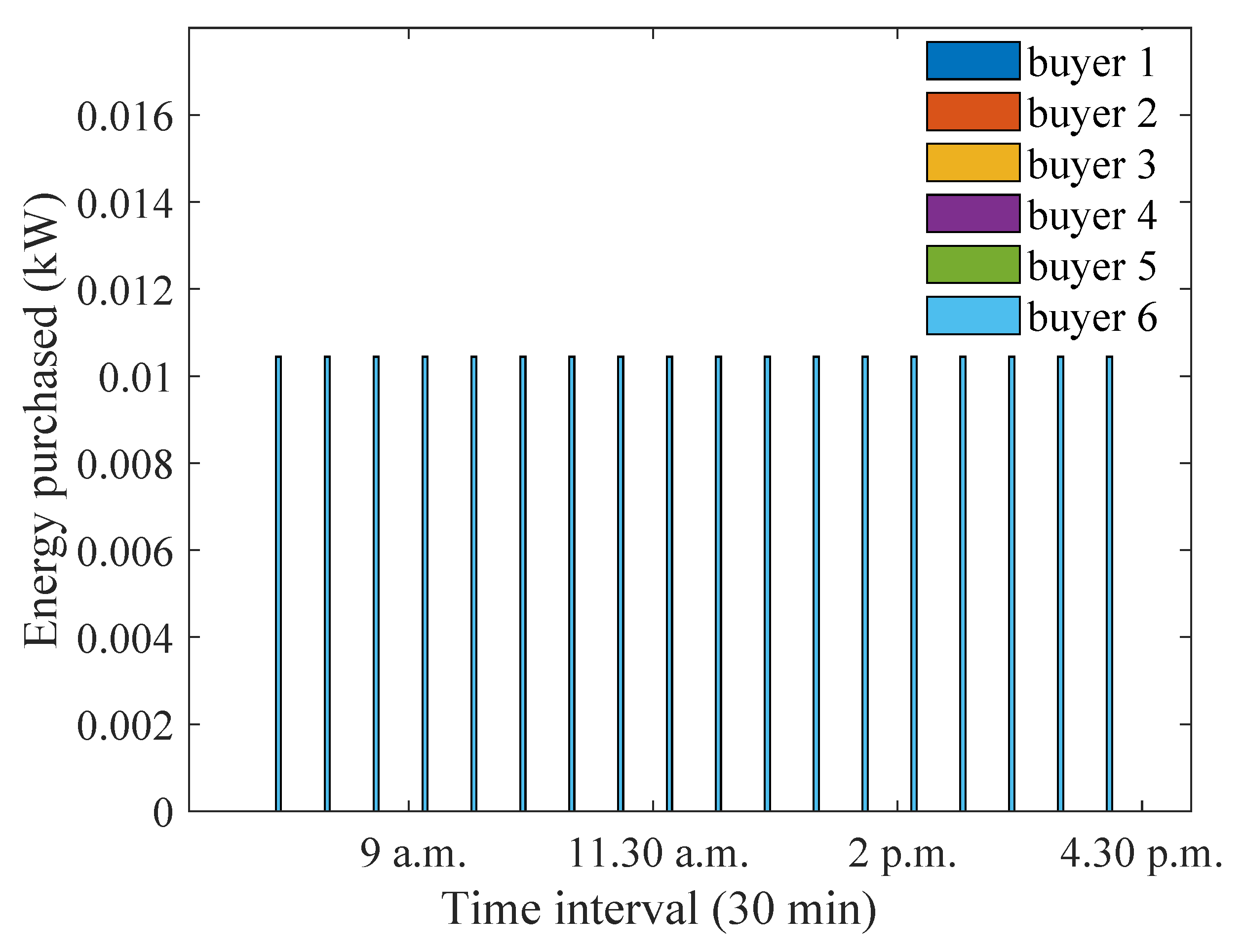
3.1. Scenario 1: Performance for Winter Data

Figure 3 shows the optimum energy sold during July 2012 when the proposed approach is implemented to optimise the preference coefficients for sellers and buyers in the P2P energy market. The evaluation is performed based on the average generation and demand data over 31 days in July 2012 for all six houses. It can be observed that trading took place between 7 a.m. and 6 p.m., when there was plenty of solar generation. It can be observed that house 1 has the highest energy sold for most of the time intervals. This is because house 1 has the highest generation capacity. House 3 sells a higher amount of energy than other houses between 9 a.m. and 2 p.m. This is because house 3 has a higher amount of energy excess during this time period. House 2 could sell energy only at 2.30 p.m., when it had a high preference coefficient.

On the other hand, Figure 4 shows the energy purchased by the buyers during the same time interval. It can be seen that buyers 5 and 6 purchased energy during all time intervals. The peak demand for houses 5 and 6 occurred at 9 a.m. and 6 p.m., respectively. However, house 2 purchased the highest amount of energy, as it had an energy deficit for most time intervals. House 4 purchased energy only at 6 p.m., when all houses except house 1 were buyers. House 1 purchased energy only during 7–8 a.m., when it did not have sufficient solar/stored energy.

Figure 5 and Figure 6 illustrate the average preference coefficients for sellers and buyers, respectively. The average preference coefficients for each seller (buyer) are computed by averaging the preference coefficient of that seller (buyer) to all buyers (sellers) in a certain time interval. House 3 has the highest preference of all buyers on average, followed by house 4. This is because house 3 and 4 have a smaller energy excess, and they are required to assign higher preference coefficients to achieve the same profit threshold. House 2 has non-zero preference coefficient only at 2.30 p.m., when it had energy excess. When considering buyers, house 3 assigned the highest preference coefficient to sellers, as it had a higher energy deficit along with a small distance from the aggregator, allowing the sellers to sell a larger amount of energy without higher losses. Houses 5 and 6 had non-zero preference coefficients for all time intervals, as they did not have any generation to support their demand.

To demonstrate the effectiveness of the proposed approach, a comparison is included in Figure 7 and Figure 8, where the sellers and buyers are preferred equally irrespective of their distances. It can be seen that the maximum energy sold ($0.009$ kW) is much smaller than that achieved when buyers are preferred based on distance ($0.02$ kW). Similar observations can be made for energy purchased values. The reason for this is that, when buyers/sellers are equally preferred, they have equal opportunities to purchase/sell from the P2P trading market. However, the energy available from a seller with larger distances will be less, because some part of it will be lost. Similarly, for buyers with larger distances, less energy will be available to consume due to losses.

3.2. Scenario 2: Impact of Excess Generation during Summer

Since excess generation can be a contributing factor for increased trading in the P2P market, the impact of increased generation during summer needs to be considered. Having more generation allows sellers to sell larger amounts of energy and buyers can have more energy available to them. Figure 9 and Figure 10 demonstrate how excess generation during summer influences the energy sold and purchased, respectively, when preference coefficients are optimised. The analysis is performed considering the generation and demand data from January 2013 averaged over 31 days. It can be observed that the highest amount of energy sold ($0.065$ kW) is higher than that in the winter month ($0.02$ kW). A similar observation can be made about the energy purchased. This is because there is excess generation during the summer months, which can be utilised for energy sale/purchase in the P2P trading market. During January, house 1 sells the highest amount of energy, as it has higher generation during the late afternoon hours when all other houses experience an energy deficit. House 5 purchases the highest amount of energy, as it has a higher demand and no generation/storage. House 1 did not need to purchase energy throughout the day as it had higher solar generation to sell in the P2P market.

Figure 11 illustrates that house 1 assigns a higher preference coefficients to buyers during early morning/late afternoon periods. On the other hand, house 4 assigns the highest preference coefficient at 9.30 a.m. This is because house 4 did not have high energy excess during this time period. Similarly, from Figure 12, houses 5 and 6 have non-zero preference coefficients during all time intervals, as these houses always have a non-zero energy deficit. Among the houses with energy generation/storage, house 3 assigns a higher preference coefficient during the late afternoon hours. This is because house 3 has a smaller energy deficit during this period and assigns a higher preference coefficient to achieve the same savings threshold. It is worth noting that buyers prefer sellers almost equally during most time intervals in summer. This is because all houses have a higher solar generation, leading to more energy being available for trading.

Figure 13 and Figure 14 show the energy sold and purchased values during the summer months when all participants are equally preferred. Similar to the proposed approach, the energy sale/purchase increased for the equally preferred sellers/buyers as well, due to the increased excess energy. The increase in the maximum amount of energy sold is 1.66 times, as compared to the winter months. On the other hand, for the proposed approach, the increase is 3.1 times. Now, seller 3 can sell energy at the same level as seller 4, and seller 2 also has an opportunity to sell energy. However, for the proposed approach, energy is sold mostly by seller 1 due to its smaller distance from the aggregator and the higher preference coefficient which is assigned to it as a result.

3.3. Scenario 3: Impact of Distances

Since the preference coefficients are optimised based on distances, it is important to identify how different settings for distances affect the optimisation outcomes. To ensure that this analysis is tractable and easily interpreted by readers, we consider two extreme examples of the distance settings. The first example sets the distance of the house closest to the aggregator to the largest possible value. The second extreme example sets the distance of the house farthest from the aggregator to the smallest possible value. Thus, in this section, we consider two sub-cases: (i) when the distance between house 1 and the aggregator is increased from $0.1$ to $0.9$ and (ii) when the distance between house 4 and the aggregator is decreased from 1 to $0.1$. Considering these two extreme cases is sufficient to identify the impact of distance on the proposed approach as it is reasonably expected that the other distance settings will result into similar trends that lie between the trends observed from the two extreme cases. It can be observed from Figure 15 that the energy sold did not change significantly when compared to Figure 3, where house 1 has a smaller distance. The only exception is during the late afternoon periods, when the amount of energy sold by house 1 is significantly smaller. This is because the distance between house 1 and the aggregator has increased. In addition, the energy sold by the other houses (e.g., house 4) increases, as these houses are more or less equally preferred due to the increased distance between house 1 and the aggregator. Similarly, it can be seen from Figure 16 that house 1 assigns a similar preference coefficient to buyers as compared to Section 3.1. This is because the distances of the buyers’ houses have not changed, meaning that house 1 can assign the same preference coefficients as before.

It can be observed from Figure 17 that the energy purchased by the buyers has increased. The maximum amount of energy is purchased by house 5, mostly during the early morning and late afternoon periods when house 1 had energy excess. Similarly, house 2 purchases an increased amount of energy at 12.30 p.m., as it has a higher demand at that time. From Figure 18, it can be seen that the maximum preference coefficients of the buyers have increased due to the increase in house 1’s distance. This is because house 1 has less energy available for buyers to purchase. However, the buyers are required to achieve the same savings threshold, and so they choose to assign a higher preference coefficient on average.

When the distance of house 4 is decreased to a smaller value, while keeping the distances of other houses same as in the scenario 1, the energy sold by house 1 decreases, while the energy sold by house 4 increases significantly, as can be seen from Figure 3 and Figure 19. This is because house 4 has a smaller distance from the aggregator. When the energy sold values are higher, a smaller preference coefficient is assigned by house 4 to achieve the same profit threshold, as can be observed from Figure 20. On the other hand, the energy purchased by house 5 increases to a higher value at 9 a.m., as can be seen from Figure 21. This is because house 5 is able to assign a higher preference coefficient to house 4, and the overall energy purchased by house 5 has an increase. It can be seen from Figure 22 that house 3 assigns a higher preference coefficient at 2 p.m. to sellers so that it can maintain its savings threshold while it purchases a smaller amount of energy.

Figure 23 and Figure 24 demonstrate how the energy sold and purchased values change, respectively, when participants are equally preferred and the distance between house 1 and the aggregator is increased. It can be observed that the overall energy sale/purchase has decreased due to higher losses at house 1. On the other hand, the energy sale/purchase values for the case when the distance between house 4 and the aggregator decreases for the equal preference case has been shown in Figure 25 and Figure 26. It is observed that house 4 now sells a higher amount of energy, as it has smaller losses, and, in effect, the energy purchase also increases due to the availability of a higher amount of energy.

3.4. Scenario 4: Impact of Profit Threshold

Since the energy sold by the sellers must satisfy the profit threshold, it is important to investigate how the setting of the profit threshold influences the trading patterns. The achievable profit threshold depends on the excess energy available at the sellers. Thus, the profit threshold cannot be increased arbitrarily, since constraints (5) and (7) will contradict each other. As a result, the maximum possible profit threshold that will not cause the violation of the constraints has been set in the simulation settings. This value has been tested through simulation, and it can also be obtained numerically based on the minimum generation values. To be specific, in this scenario, the profit threshold of the sellers is increased to a value of $0.003$ AUD. It can be observed from Figure 27 that the energy sold by the sellers increases to a larger value, especially during the early morning/late afternoon hours. This is because the sellers need to sell a higher amount of energy to achieve a higher profit threshold. It can be noted that during 5–6 p.m., only house 1 is able to sell energy, whereas, with a smaller profit threshold, both houses 1 and 4 were selling energy. This is because house 4 did not have sufficient energy to achieve the increased profit threshold. As a result, the required energy is obtained from house 1 alone. The preference coefficients of the sellers do not change significantly apart from the early morning/late afternoon periods, as seen from Figure 28. During 7–8 a.m., house 4 has a higher preference coefficient to ensure that it achieves the required profit threshold. For similar reasons, house 1 has a higher preference coefficient at 6 p.m.

From Figure 29, it can be seen that most buyers have an increased energy purchase due to the higher availability of energy from the sellers. For houses 1 and 4, the increase is not observed, because they have a smaller energy deficit as compared to other houses and can achieve the savings threshold even with a smaller energy purchase. The average preference coefficients of all buyers increase when the profit threshold is increased, as seen from Figure 30. This is because a higher amount of energy is available to the buyers as compared to that available in scenario 1. However, the maximum preference coefficient of buyer 3 has increased at 2 p.m., which can be attributed to its lower distance from the aggregator, and, for the same level of energy deficit, a higher preference coefficient is assigned to utilise the higher amount of energy excess from the sellers.

Figure 31 and Figure 32 show the impact of an increased profit threshold on the energy sold and purchased values for the equally preferred participants. As expected from previous discussions, the energy sold increases so that the sellers can achieve the higher profit threshold. Due to the increased availability of energy, the energy purchase also increases. It can be noted that, for the equal preference case, the energy sold values are more or less equal for all sellers, irrespective of their distances. This is because all houses are equally preferred, and, when the profit threshold is set to a higher value, all sellers aim to sell as much energy as possible to achieve that profit threshold.

3.5. Summary of the Simulation Results

To summarise the aforementioned findings, it can be observed that the proposed approach, which applies unequal priority coefficients to energy sold/purchased from different users, outperforms the equal preference based approach. This is because the proposed approach takes into account the distances between the users and the aggregator, while the existing approach does not. The increased generation during summer results in increased trading for both approaches. However, the sold/purchased energy is still higher for the proposed approach. The two extreme cases for measuring the impact of distance lead to the fact that the energy sold by a seller decreases with distance when there are other sellers with a sufficient amount of energy to satisfy the demand at that time. When the existing and proposed approaches are compared, the existing approach has an overall smaller amount of energy sold, due to higher losses for users with increased distance. On the other hand, the proposed approach adapts the optimisation based on the fact that some users have higher distances, and, as a result, another seller needs to be preferred. With the increase in profit threshold, it can be observed that sellers are now able to sell more energy to achieve the increased profit threshold, though the increase is higher for the proposed approach in comparison to the existing approach. Thus, the aforementioned comparison clearly shows that the proposed approach outperforms the existing approach for all designed scenarios.

4. Discussion of Key Findings

In this section, we highlight the key findings of the proposed research that has emerged from the evaluation of the case study and relate these to the relevant literature. From a technical perspective, the proposed method has been able to achieve an increased energy sale/purchase in the P2P trading market by ensuring that users with smaller distances are preferred more by sellers and buyers. It can also be observed that the increased excess generation during the summer months will further increase the benefits of P2P trading, which can be a motivating factor for potential participants and used to develop marketing strategies accordingly. The preference coefficients vary for users with different distances mainly during periods of lower solar generation and when sellers do not have sufficient energy excess. This can motivate the design of different pricing signals and can be integrated further to enhance the economic aspects of the P2P trading mechanism. Another key finding is that sellers with larger distances aim to sell more energy as they are assigned a smaller preference coefficient, and they still want to achieve the same profit threshold similar to sellers with smaller distances. This fact can inform the selection of the trading prices by the sellers with larger distances.

The findings from the proposed study can be compared with [25,28], which are relevant studies which consider the impact of distance-based priorities in P2P energy trading. The authors in [25] combine the total energy sale/purchase information as traded energy and statistically represent the amount of energy traded. However, the energy trading information for different time slots is not available. In [28], the authors demonstrate the power flow for individual participants only during selected time slots. Moreover, the overall profit/savings of the participants are illustrated. The system losses due to distances between prosumers as well as the resulting voltage profiles are shown in [27], but the energy sale/purchase is not presented. Similarly, in [26], the costs for individual participants over the entire day are shown without demonstrating the energy sale/purchase profiles. On the other hand, the proposed work adds value to these findings by including information on how much energy is sold/purchased by individual houses throughout the entire trading period. This information will be more suitable for identifying individual participant strategies regarding P2P energy trading.

Apart from these technical aspects, there are a number of managerial implications of this study, which apply to the regulatory bodies and utilities. For example, since participants with larger distances have a reduced opportunity to achieve profit/savings from the P2P market, more incentives could be provided to them so that users with larger distances are also encouraged to participate. In addition, the market structure can be designed in such a way that the preference coefficients are applied during periods of high variation in generation or demand, and, during other times, the participants will be equally preferred. This will help utilise the benefits of the proposed approach in the best possible way. From the utility perspectives, the pricing strategies can be designed for users participating in P2P energy trading considering the seasonal variations in excess generation, which largely influence how much the participants will depend on the utility grid to achieve a supply/demand balance.

In addition, the social implications of the proposed approach can be significant. P2P energy trading in general establishes a sense of energy independence among the participating users and enhances their decision-making capacities from energy sale/purchase perspectives. The proposed approach assigns smaller scaling factors to the energy sold/purchased values of the participants with larger distances. In this way, users with larger distances still have the opportunity to participate in the market while ensuring other users are not impacted by the losses caused by energy sale/purchase with users at larger distances. This essentially enhances the social bonding between different community groups but not at the cost of decreased profit/savings. The outcomes of this study will help individual participants to design strategies for maximising their profits/savings from P2P energy trading by identifying prices and understanding the trends in the P2P market. As a result, user awareness of energy consumption and sustainable energy use practices is expected to rise, which will improve the socioeconomic status of the participants. The proposed approach can also lead to the generation of local jobs for maintaining the energy management systems and installing solar panels, as well as integrating the web-based systems. Future research on this method can innovate new strategies for cost and profit sharing and investigate the fairness aspects of the P2P trading mechanism.

5. Conclusions

This paper has investigated an optimisation approach which assigns higher preferences to participants with smaller distances from the aggregator. The proposed approach allows each seller/buyer to optimise the preference coefficient for each buyer/seller along with energy to be sold/purchased. Given that users with larger distances can cause more power losses in the P2P trading network, it is essential to scale down their energy sale/purchase values to ensure an efficient trading mechanism. In comparison to the case when all participants are preferred equally, the proposed approach achieves a higher energy sold/purchased for P2P trading. For the considered case study, this improvement is more than two times. It can also be observed that the sellers sell 3 times higher amounts of energy during summer months in comparison to the winter months. However, when the distance of a seller increases, the buyers assign a lower preference coefficient, and, as a result, the seller offers a higher amount of energy to maintain its profit threshold. Future work will focus on integrating different pricing models and auction mechanisms with the preference coefficient optimisation approach. The findings from this study will allow participants to optimise their pricing strategies considering the impact of other users’ preferences and energy consumption trends.

References

1. Ostergaard, J.; Ziras, C.; Bindner, H.W.; Kazempour, J.; Marinelli, M.; Markussen, P.; Rosted, S.H.; Christensen, J.S. Energy Security Through Demand-Side Flexibility: The Case of Denmark. IEEE Power Energy Mag. 2021, 19, 46–55. [Google Scholar] [CrossRef]
2. Zhang, C.; Wu, J.; Zhou, Y.; Cheng, M.; Long, C. Peer-to-Peer energy trading in a Microgrid. Appl. Energy 2018, 220, 1–12. [Google Scholar] [CrossRef]
3. Feed-in Tariff (FIT) Generation & Export Payment Rate Table. 2019. Available online: https://www.ofgem.gov.uk/sites/default/files/docs/2016/07/tariff_tables_july_2016.pdf (accessed on 20 February 2022).
4. Trivedi, R.; Patra, S.; Sidqi, Y.; Bowler, B.; Zimmermann, F.; Deconinck, G.; Papaemmanouil, A.; Khadem, S. Community-Based Microgrids: Literature Review and Pathways to Decarbonise the Local Electricity Network. Energies 2022, 15, 918. [Google Scholar] [CrossRef]
5. Islam, S.N. A New Pricing Scheme for Intra-Microgrid and Inter-Microgrid Local Energy Trading. Electronics 2019, 8, 898. [Google Scholar] [CrossRef] [Green Version]
6. Tushar, W.; Saha, T.K.; Yuen, C.; Smith, D.; Poor, H.V. Peer-to-Peer Trading in Electricity Networks: An Overview. IEEE Trans. Smart Grid 2020, 11, 3185–3200. [Google Scholar] [CrossRef] [Green Version]
7. Karami, M.; Madlener, R. Business models for peer-to-peer energy trading in Germany based on households’ beliefs and preferences. Appl. Energy 2022, 306, 118053. [Google Scholar] [CrossRef]
8. Ableitner, L.; Tiefenbeck, V.; Meeuw, A.; Wörner, A.; Fleisch, E.; Wortmann, F. User behavior in a real-world peer-to-peer electricity market. Appl. Energy 2020, 270, 115061. [Google Scholar] [CrossRef]
9. Klein, L.P.; Matos, L.M.; Allegretti, G. A pragmatic approach towards end-user engagement in the context of peer-to-peer energy sharing. Energy 2020, 205, 118001. [Google Scholar] [CrossRef]
10. Guerrero, J.; Gebbran, D.; Mhanna, S.; Chapman, A.C.; Verbič, G. Towards a transactive energy system for integration of distributed energy resources: Home energy management, distributed optimal power flow, and peer-to-peer energy trading. Renew. Sustain. Energy Rev. 2020, 132, 110000. [Google Scholar] [CrossRef]
11. Paudel, A.; Chaudhari, K.; Long, C.; Gooi, H.B. Peer-to-Peer Energy Trading in a Prosumer-Based Community Microgrid: A Game-Theoretic Model. IEEE Trans. Ind. Electron. 2019, 66, 6087–6097. [Google Scholar] [CrossRef]
12. Tushar, W.; Yuen, C.; Mohsenian-Rad, H.; Saha, T.; Poor, H.V.; Wood, K.L. Transforming Energy Networks via Peer-to-Peer Energy Trading: The Potential of Game-Theoretic Approaches. IEEE Signal Process. Mag. 2018, 35, 90–111. [Google Scholar] [CrossRef] [Green Version]
13. Chen, K.; Lin, J.; Song, Y. Trading strategy optimisation for a prosumer in continuous double auction-based peer-to-peer market: A prediction-integration model. Appl. Energy 2019, 242, 1121–1133. [Google Scholar] [CrossRef]
14. Luo, F.; Dong, Z.Y.; Liang, G.; Murata, J.; Xu, Z. A Distributed Electricity Trading System in Active Distribution Networks Based on Multi-Agent Coalition and Blockchain. IEEE Trans. Power Syst. 2019, 34, 4097–4108. [Google Scholar] [CrossRef]
15. Islam, S.N.; Mahmud, M.A.; Oo, A.M.T. A Communication Scheme for Blockchain based Peer to Peer Energy Trading. In Proceedings of the 2020 IEEE Power Energy Society General Meeting (PESGM), Montreal, QC, Canada, 2–6 August 2020; pp. 1–5. [Google Scholar] [CrossRef]
16. Mahmud, A.; Islam, S.N.; Lilley, I. A Smart Energy Hub for Smart Cities: Enabling Peer-to-Peer Energy Sharing and Trading. IEEE Consum. Electron. Mag. 2021, 10, 97–105. [Google Scholar] [CrossRef]
17. Khorasany, M.; Mishra, Y.; Ledwich, G. A Decentralized Bilateral Energy Trading System for Peer-to-Peer Electricity Markets. IEEE Trans. Ind. Electron. 2020, 67, 4646–4657. [Google Scholar] [CrossRef] [Green Version]
18. Morstyn, T.; Teytelboym, A.; Mcculloch, M.D. Bilateral Contract Networks for Peer-to-Peer Energy Trading. IEEE Trans. Smart Grid 2019, 10, 2026–2035. [Google Scholar] [CrossRef]
19. Kim, H.; Lee, J.; Bahrami, S.; Wong, V.W.S. Direct Energy Trading of Microgrids in Distribution Energy Market. IEEE Trans. Power Syst. 2020, 35, 639–651. [Google Scholar] [CrossRef]
20. Paudel, A.; Sampath, L.P.M.I.; Yang, J.; Gooi, H.B. Peer-to-Peer Energy Trading in Smart Grid Considering Power Losses and Network Fees. IEEE Trans. Smart Grid 2020, 11, 4727–4737. [Google Scholar] [CrossRef]
21. Chakraborty, S.; Baarslag, T.; Kaisers, M. Automated peer-to-peer negotiation for energy contract settlements in residential cooperatives. Appl. Energy 2020, 259, 114173. [Google Scholar] [CrossRef] [Green Version]
22. Jogunola, O.; Wang, W.; Adebisi, B. Prosumers Matching and Least-Cost Energy Path Optimisation for Peer-to-Peer Energy Trading. IEEE Access 2020, 8, 95266–95277. [Google Scholar] [CrossRef]
23. Khorasany, M.; Mishra, Y.; Ledwich, G. Peer-to-peer market clearing framework for DERs using knapsack approximation algorithm. In Proceedings of the 2017 IEEE PES Innovative Smart Grid Technologies Conference Europe (ISGT-Europe), Torino, Italy, 26–29 September 2017; pp. 1–6. [Google Scholar]
24. Moret, F.; Pinson, P.; Papakonstantinou, A. Heterogeneous risk preferences in community-based electricity markets. Eur. J. Oper. Res. 2020, 287, 36–48. [Google Scholar] [CrossRef]
25. Guerrero, J.; Sok, B.; Chapman, A.C.; Verbič, G. Electrical-distance driven peer-to-peer energy trading in a low-voltage network. Appl. Energy 2021, 287, 116598. [Google Scholar] [CrossRef]
26. Chang, X.; Xu, Y.; Sun, H. Vertex scenario-based robust peer-to-peer transactive energy trading in distribution networks. Int. J. Electr. Power Energy Syst. 2022, 138, 107903. [Google Scholar] [CrossRef]
27. Iqbal, S.; Nasir, M.; Zia, M.F.; Riaz, K.; Sajjad, H.; Khan, H.A. A novel approach for system loss minimization in a peer-to-peer energy sharing community DC microgrid. Int. J. Electr. Power Energy Syst. 2021, 129, 106775. [Google Scholar] [CrossRef]
28. Malik, S.; Duffy, M.; Thakur, S.; Hayes, B.; Breslin, J. A priority-based approach for peer-to-peer energy trading using cooperative game theory in local energy community. Int. J. Electr. Power Energy Syst. 2022, 137, 107865. [Google Scholar] [CrossRef]
29. Sebastian, A.J.; Islam, S.N.; Mahmud, A.; Oo, A.M.T. Optimum Local Energy Trading considering Priorities in a Microgrid. In Proceedings of the 2019 IEEE International Conference on Communications, Control, and Computing Technologies for Smart Grids (SmartGridComm), Beijing, China, 21–23 October 2019; pp. 1–6. [Google Scholar]
30. Morstyn, T.; McCulloch, M.D. Multiclass Energy Management for Peer-to-Peer Energy Trading Driven by Prosumer Preferences. IEEE Trans. Power Syst. 2019, 34, 4005–4014. [Google Scholar] [CrossRef]
31. Lofberg, J. YALMIP: A toolbox for modeling and optimisation in MATLAB. In Proceedings of the 2004 IEEE International Conference on Robotics and Automation (IEEE Cat. No.04CH37508), New Orleans, LA, USA, 26 April–1 May 2004; pp. 284–289. [Google Scholar]
32. Ausgrid. Solar Home Electricity Data. Available online: https://www.ausgrid.com.au/Industry/Our-Research/Data-to-share/Solar-home-electricity-data (accessed on 10 March 2022).
Figure 1. Optimisation of preference coefficients at sellers and buyers.
Energies 15 04212 g001
Figure 2. Illustration of the considered P2P trading network structure in the case study.
Energies 15 04212 g002
Figure 3. Optimum energy sold during winter months.
Energies 15 04212 g003
Figure 4. Optimum energy purchased during winter months.
Energies 15 04212 g004
Figure 5. Optimum preference coefficients for sellers during winter months.
Energies 15 04212 g005
Figure 6. Optimum preference coefficients for buyers during winter months.
Energies 15 04212 g006
Figure 7. Optimum energy sold for equally preferred sellers and buyers during winter months.
Energies 15 04212 g007
Figure 8. Optimum energy purchased for equally preferred sellers and buyers during winter months.
Energies 15 04212 g008
Figure 9. Optimum energy sold for sellers during summer months.
Energies 15 04212 g009
Figure 10. Optimum energy purchased for buyers during summer months.
Energies 15 04212 g010
Figure 11. Optimum preference coefficients for sellers during summer months.
Energies 15 04212 g011
Figure 12. Optimum preference coefficients for buyers during summer months.
Energies 15 04212 g012
Figure 13. Optimum energy sold for equally preferred sellers and buyers during summer months.
Energies 15 04212 g013
Figure 14. Optimum energy purchased for equally preferred sellers and buyers during summer months.
Energies 15 04212 g014
Figure 15. Optimum energy sold when distance between house 1 and the aggregator is increased.
Energies 15 04212 g015
Figure 16. Optimum preference coefficients for sellers when distance between house 1 and the aggregator is increased.
Energies 15 04212 g016
Figure 17. Optimum energy purchased when distance between house 1 and the aggregator is increased.
Energies 15 04212 g017
Figure 18. Optimum preference coefficients for buyers when distance between house 1 and the aggregator is increased.
Energies 15 04212 g018
Figure 19. Optimum energy sold when distance between house 4 and the aggregator is decreased.
Energies 15 04212 g019
Figure 20. Optimum preference coefficients for sellers when distance between house 4 and the aggregator is decreased.
Energies 15 04212 g020
Figure 21. Optimum energy purchased when distance between house 4 and the aggregator is decreased.
Energies 15 04212 g021
Figure 22. Optimum preference coefficients for buyers when distance between house 4 and the aggregator is decreased.
Energies 15 04212 g022
Figure 23. Optimum energy sold for equally preferred sellers and buyers when distance between house 1 and the aggregator is increased.
Energies 15 04212 g023
Figure 24. Optimum energy purchased for equally preferred sellers and buyers when distance between house 1 and the aggregator is increased.
Energies 15 04212 g024
Figure 25. Optimum energy sold for equally preferred sellers and buyers when distance between house 4 and the aggregator is decreased.
Energies 15 04212 g025
Figure 26. Optimum energy purchased for equally preferred sellers and buyers when distance between house 4 and the aggregator is decreased.
Energies 15 04212 g026
Figure 27. Optimum energy sold when profit threshold is increased to a larger value.
Energies 15 04212 g027
Figure 28. Optimum preference coefficients for sellers when profit threshold is increased to a larger value.
Energies 15 04212 g028
Figure 29. Optimum energy purchased when profit threshold is increased to a larger value.
Energies 15 04212 g029
Figure 30. Optimum preference coefficients for buyers when profit threshold is increased to a larger value.
Energies 15 04212 g030
Figure 31. Optimum energy sold for equally preferred sellers and buyers when when profit threshold is increased to a larger value.
Energies 15 04212 g031
Figure 32. Optimum energy purchased for equally preferred sellers and buyers when profit threshold is increased to a larger value.
Energies 15 04212 g032