
BIPV Modeling with Artificial Neural Networks: Towards a BIPV Digital Twin


Abstract
:
1. Introduction
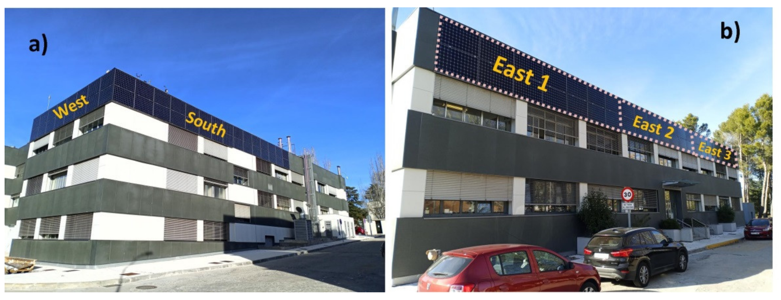
2. Description of the BIPV Arrays under Study
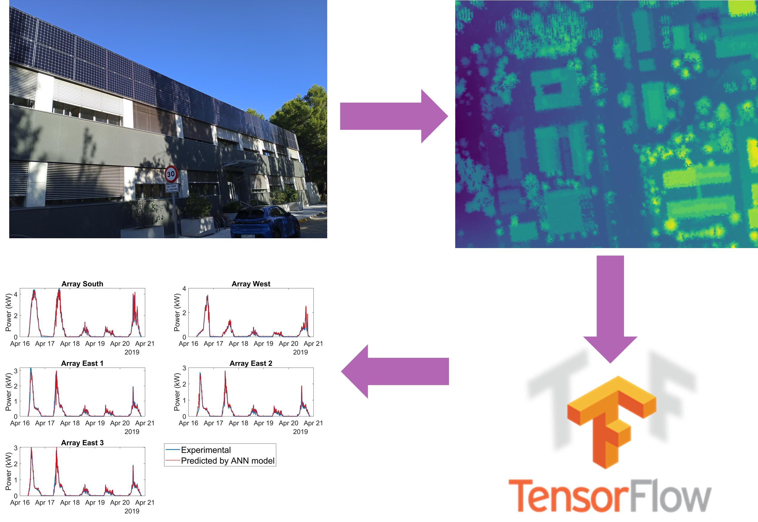
3. Methodology
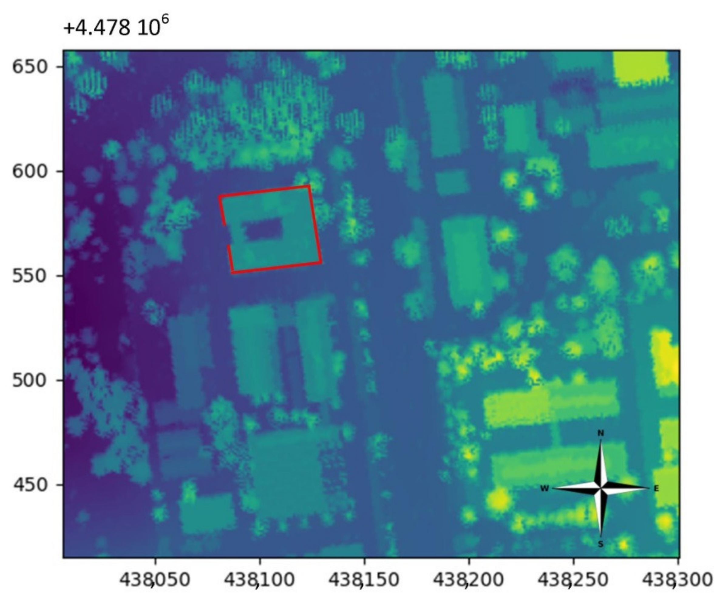
3.1. Computation of Shading Parameters
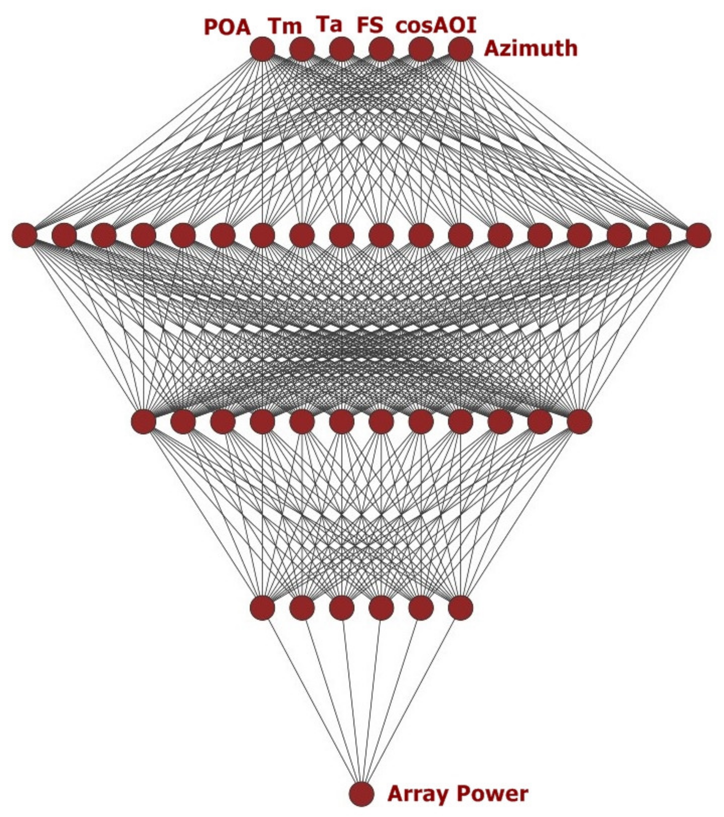
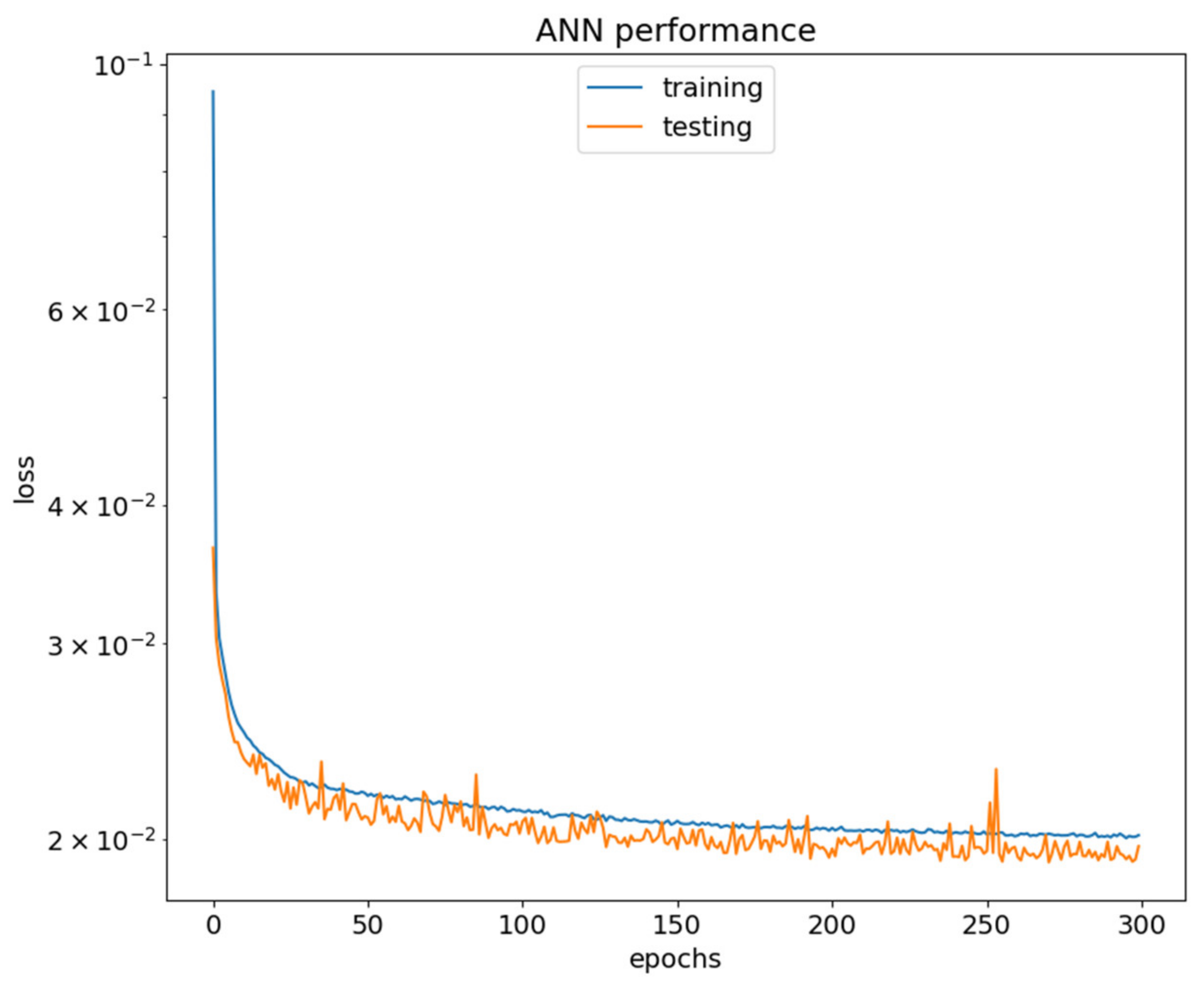
3.2. Artificial Neural Network (ANN)
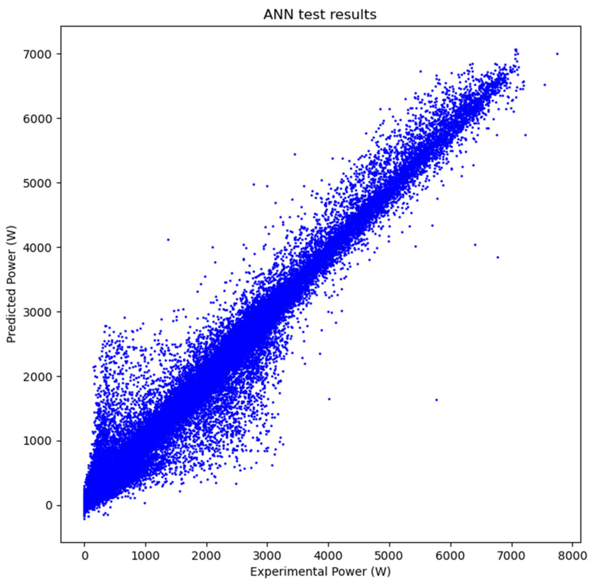
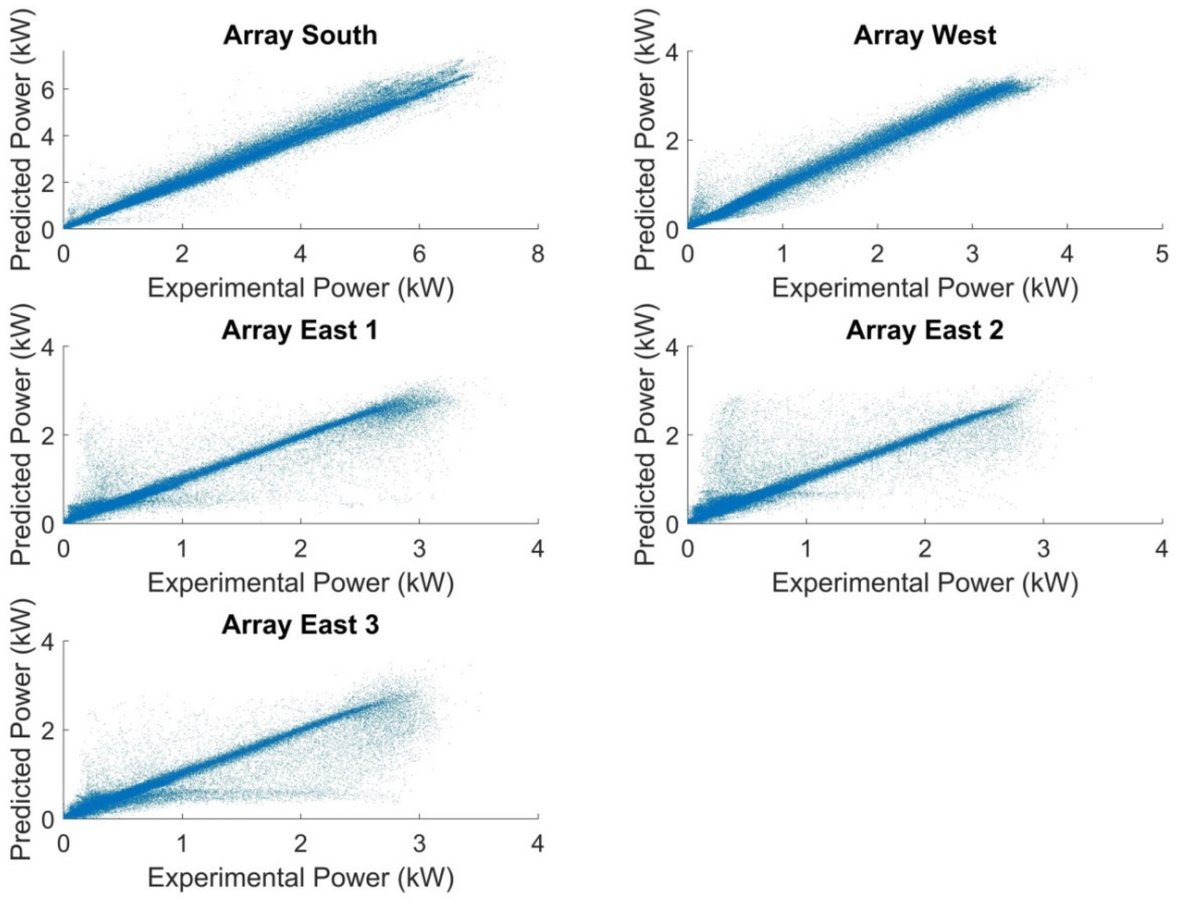
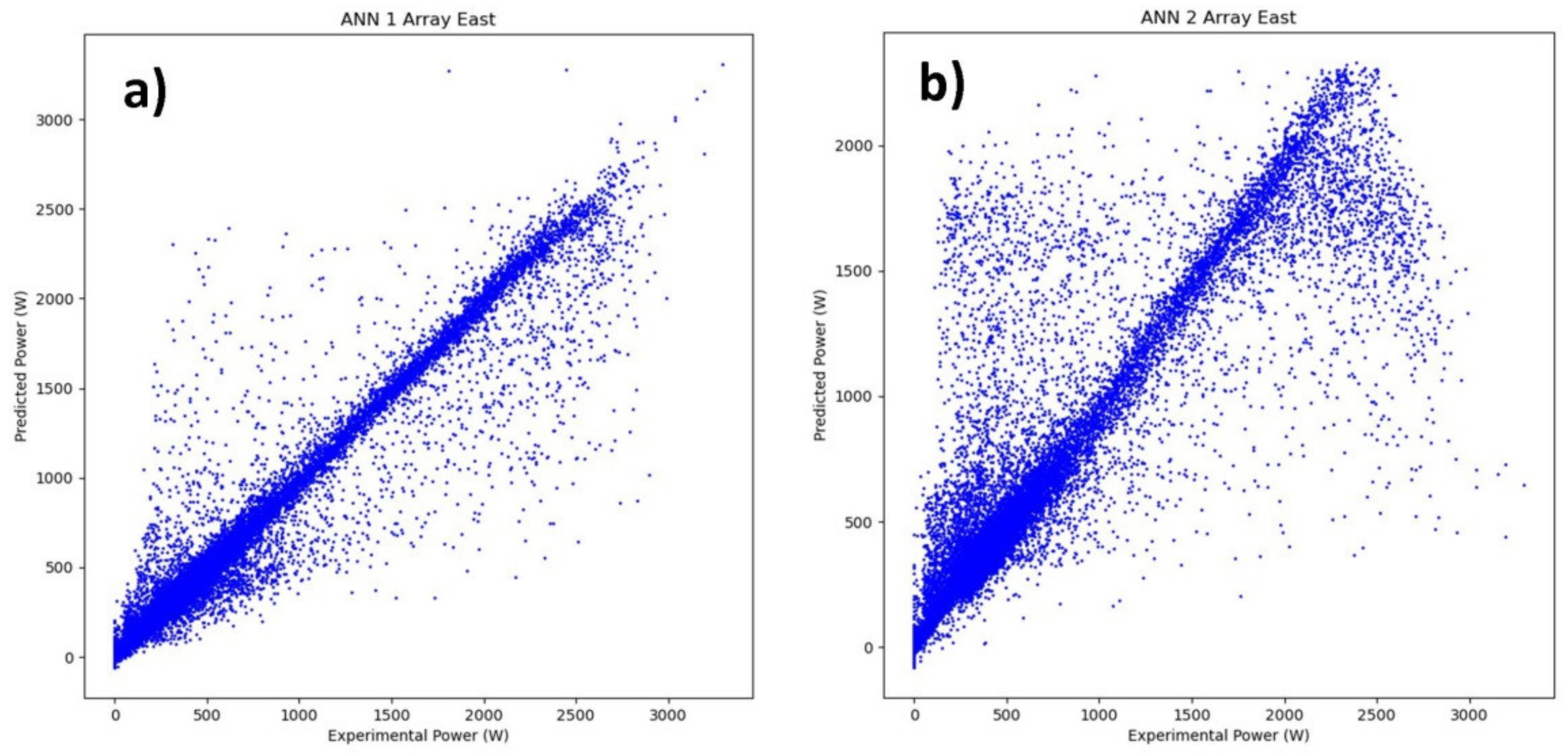
4. Results
5. Conclusions
Author Contributions
Funding
Institutional Review Board Statement
Informed Consent Statement
Data Availability Statement
Acknowledgments
Conflicts of Interest
Nomenclature
| ANN | Artificial Neural Network |
| BAPV | Building Applied Photovoltaics |
| BIPV | Building Integrated Photovoltaics |
| DSM | Digital Surface Model |
| DT | Digital Twin |
| LIDAR | Laser Imaging Detection and Ranging |
| PV | Photovoltaic |
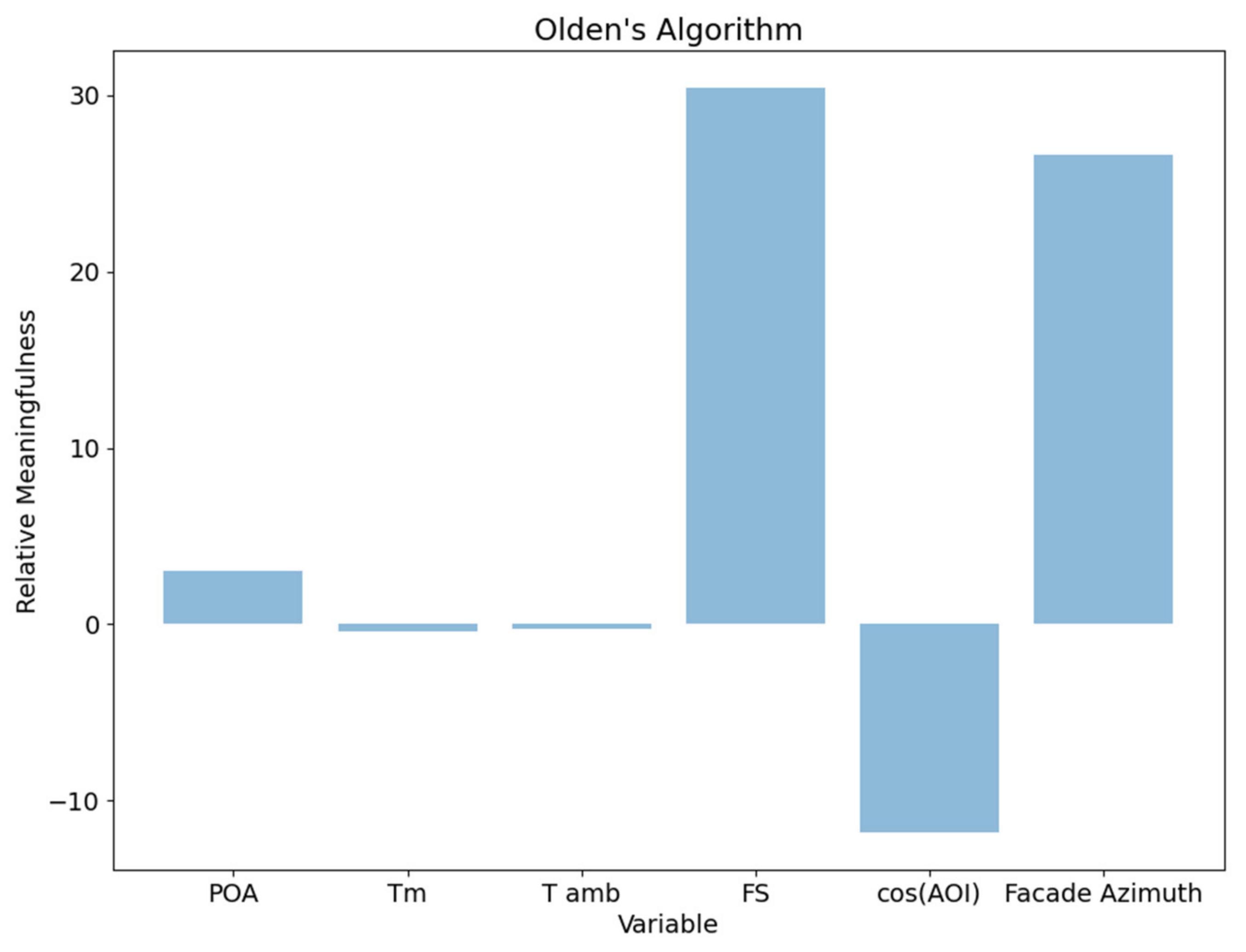
| cosAOI | cosine of the sunlight incident angle |
| FS | illuminated fraction of array |
| MAE | mean absolute error |
| MBE | mean bias error |
| POA | plane of array irradiance |
| R2 | coefficient of determination |
| RMSE | root mean square error |
| Ta | ambient temperature |
| Tm | module temperature |
References
- Asmelash, E.; Prakash, G. Future of Solar Photovoltaic: Deployment, Investment, Technology, Grid Integration and Socio-Economic Aspects; A Global Energy Transformation: Paper; IRENA: Bonn, Germany, 2019; ISBN 9789292601553. [Google Scholar]
- Liu, Z.; Zhang, Y.; Yuan, X.; Liu, Y.; Xu, J.; Zhang, S.; He, B.J. A Comprehensive Study of Feasibility and Applicability of Building Integrated Photovoltaic (BIPV) Systems in Regions with High Solar Irradiance. J. Clean. Prod. 2021, 307, 127240. [Google Scholar] [CrossRef]
- Ghosh, A. Potential of Building Integrated and Attached/Applied Photovoltaic (BIPV/BAPV) for Adaptive Less Energy-Hungry Building’s Skin: A Comprehensive Review. J. Clean. Prod. 2020, 276, 123343. [Google Scholar] [CrossRef]
- Gurupira, T.; Rix, A.J. PV Simulation Software Comparisons: Pvsyst, Nrel Sam and Pvlib. In Proceedings of the 25th Southern African Universities Power Engineering Conference (SAUPEC 2017), Stellenbosch, South Africa, 30 January–1 February 2017. [Google Scholar]
- Jakica, N.; Ynag, R.J.; Eisenlohr, J. BIPV Design and Performance Modelling: Tools and Methods; Report IEA-PVPS T15-09:2019; International Energy Agency: Paris, France, 2019; ISBN 9783906042862. [Google Scholar]
- Martín-Chivelet, N.; Kapsis, K.; Wilson, H.R.; Delisle, V.; Yang, R.; Olivieri, L.; Polo, J.; Eisenlohr, J.; Roy, B.; Maturi, L.; et al. Building-Integrated Photovoltaic (BIPV) Products and Systems: A Review of Energy-Related Behavior. Energy Build. 2022, 262, 111998. [Google Scholar] [CrossRef]
- Celik, B.; Karatepe, E.; Silvestre, S.; Gokmen, N.; Chouder, A. Analysis of Spatial Fixed PV Arrays Configurations to Maximize Energy Harvesting in BIPV Applications. Renew. Energy 2015, 75, 534–540. [Google Scholar] [CrossRef] [Green Version]
- Desthieux, G.; Carneiro, C.; Camponovo, R.; Ineichen, P.; Morello, E.; Boulmier, A.; Abdennadher, N.; Dervey, S.; Ellert, C. Solar Energy Potential Assessment on Rooftops and Facades in Large Built Environments Based on Lidar Data, Image Processing, and Cloud Computing. Methodological Background, Application, and Validation in Geneva (Solar Cadaster). Front. Built Environ. 2018, 4, 14. [Google Scholar] [CrossRef]
- Revesz, M.; Zamini, S.; Oswald, S.M.; Trimmel, H.; Weihs, P. SEBEpv—New Digital Surface Model Based Method for Estimating the Ground Reflected Irradiance in an Urban Environment. Sol. Energy 2020, 199, 400–410. [Google Scholar] [CrossRef]
- Dorman, M.; Erell, E.; Vulkan, A.; Kloog, I. Shadow: R Package for Geometric Shadow Calculations in an Urban Environment. R J. 2020, 11, 287. [Google Scholar] [CrossRef] [Green Version]
- Freitas, S.; Catita, C.; Redweik, P.; Brito, M.C. Modelling Solar Potential in the Urban Environment: State-of-the-Art Review. Renew. Sustain. Energy Rev. 2015, 41, 915–931. [Google Scholar] [CrossRef]
- De Sousa Freitas, J.; Cronemberger, J.; Soares, R.M.; Amorim, C.N.D. Modeling and Assessing BIPV Envelopes Using Parametric Rhinoceros Plugins Grasshopper and Ladybug. Renew. Energy 2020, 160, 1468–1479. [Google Scholar] [CrossRef]
- Landelius, T.; Andersson, S.; Abrahamsson, R. Modelling and Forecasting PV Production in the Absence of Behind-the-Meter Measurements. Prog. Photovolt. Res. Appl. 2019, 27, 990–998. [Google Scholar] [CrossRef] [Green Version]
- Ahmed, R.; Sreeram, V.; Mishra, Y.; Arif, M.D. A Review and Evaluation of the State-of-the-Art in PV Solar Power Forecasting: Techniques and Optimization. Renew. Sustain. Energy Rev. 2020, 124, 109792. [Google Scholar] [CrossRef]
- Zhou, Y.; Zhou, N.; Gong, L.; Jiang, M. Prediction of Photovoltaic Power Output Based on Similar Day Analysis, Genetic Algorithm and Extreme Learning Machine. Energy 2020, 204, 117894. [Google Scholar] [CrossRef]
- Ağbulut, Ü.; Gürel, A.E.; Ergün, A.; Ceylan, İ. Performance Assessment of a V-Trough Photovoltaic System and Prediction of Power Output with Different Machine Learning Algorithms. J. Clean. Prod. 2020, 268, 122269. [Google Scholar] [CrossRef]
- Behera, M.K.; Majumder, I.; Nayak, N. Solar Photovoltaic Power Forecasting Using Optimized Modified Extreme Learning Machine Technique. Eng. Sci. Technol. Int. J. 2018, 21, 428–438. [Google Scholar] [CrossRef]
- Wang, F.; Xuan, Z.; Zhen, Z.; Li, K.; Wang, T.; Shi, M. A Day-Ahead PV Power Forecasting Method Based on LSTM-RNN Model and Time Correlation Modification under Partial Daily Pattern Prediction Framework. Energy Convers. Manag. 2020, 212, 112766. [Google Scholar] [CrossRef]
- Mittal, M.; Bora, B.; Saxena, S.; Gaur, A.M. Performance Prediction of PV Module Using Electrical Equivalent Model and Artificial Neural Network. Sol. Energy 2018, 176, 104–117. [Google Scholar] [CrossRef]
- Almonacid, F.; Rus, C.; Pérez, P.J.; Hontoria, L. Estimation of the Energy of a PV Generator Using Artificial Neural Network. Renew. Energy 2009, 34, 2743–2750. [Google Scholar] [CrossRef]
- Almonacid, F.; Rus, C.; Pérez-Higueras, P.; Hontoria, L. Calculation of the Energy Provided by a PV Generator. Comparative Study: Conventional Methods vs. Artificial Neural Networks. Energy 2011, 36, 375–384. [Google Scholar] [CrossRef]
- Mellit, A.; Kalogirou, S. Assessment of Machine Learning and Ensemble Methods for Fault Diagnosis of Photovoltaic Systems. Renew. Energy 2021, 184, 1074–1090. [Google Scholar] [CrossRef]
- Kara Mostefa Khelil, C.; Amrouche, B.; Kara, K.; Chouder, A. The Impact of the ANN’s Choice on PV Systems Diagnosis Quality. Energy Convers. Manag. 2021, 240, 114278. [Google Scholar] [CrossRef]
- Arafet, K.; Berlanga, R. Digital Twins in Solar Farms: An Approach through Time Series and Deep Learning. Algorithms 2021, 14, 156. [Google Scholar] [CrossRef]
- Razo, D.E.G.; Müller, B.; Madsen, H.; Wittwer, C. A Genetic Algorithm Approach as a Self-Learning and Optimization Tool for PV Power Simulation and Digital Twinning. Energies 2020, 13, 6712. [Google Scholar] [CrossRef]
- Alanne, K.; Sierla, S. An Overview of Machine Learning Applications for Smart Buildings. Sustain. Cities Soc. 2022, 76, 103445. [Google Scholar] [CrossRef]
- Kabilan, R.; Chandran, V.; Yogapriya, J.; Karthick, A.; Gandhi, P.P.; Mohanavel, V.; Rahim, R.; Manoharan, S. Short-Term Power Prediction of Building Integrated Photovoltaic (BIPV) System Based on Machine Learning Algorithms. Int. J. Photoenergy 2021, 2021, 5582418. [Google Scholar] [CrossRef]
- Polo, J.; Martín-Chivelet, N.; Alonso-Abella, M.; Alonso-García, C. Photovoltaic Generation on Vertical Façades in Urban Context from Open Satellite-Derived Solar Resource Data. Solar Energy 2021, 224, 1396–1405. [Google Scholar] [CrossRef]
- Martín-Chivelet, N.; Gutiérrez, J.C.; Alonso-Abella, M.; Chenlo, F.; Cuenca, J. Building Retrofit with Photovoltaics: Construction and Performance of a BIPV Ventilated Façade. Energies 2018, 11, 1719. [Google Scholar] [CrossRef] [Green Version]
- Lindberg, F.; Jonsson, P.; Honjo, T.; Wästberg, D. Solar Energy on Building Envelopes—3D Modelling in a 2D Environment. Sol. Energy 2015, 115, 369–378. [Google Scholar] [CrossRef]
- Catita, C.; Redweik, P.; Pereira, J.; Brito, M.C.C. Extending Solar Potential Analysis in Buildings to Vertical Facades. Comput. Geosci. 2014, 66, 1–12. [Google Scholar] [CrossRef]
- Géron, A. Hands-On Machine Learning with Scikit-Learn and TensorFlow; O’Reilly Media: Newton, MA, USA, 2017; ISBN 9781491962299. [Google Scholar]
- Holmgren, W.F.; Hansen, C.H.; Mikofski, M.A. Pvlib Python: A Python Package for Modeling Solar Energy Systems. J. Open Source Softw. 2018, 3, 884. [Google Scholar] [CrossRef] [Green Version]
- Olden, J.D.; Joy, M.K.; Death, R.G. An Accurate Comparison of Methods for Quantifying Variable Importance in Artificial Neural Networks Using Simulated Data. Ecol. Model. 2004, 178, 389–397. [Google Scholar] [CrossRef]


| Array | Azimuth (°) | Configuration | Module Model | Power (W) | Inverter Model | Inverter Power (kW) |
|---|---|---|---|---|---|---|
| South | 172.3 | 7sx4p | SunPower E18-325 | 305 | Fronius IG Plus 100 V-3 | 8 |
| West | 262.3 | 8sx2p | SunPower E20-327 | 327 | Fronius IG Plus 50 V-1 | 4 |
| East 1 | 82.3 | 7sx2p | SunPower E20-327 | 327 | Fronius IG Plus 50 V-1 | 4 |
| East 2 | 82.3 | 7sx2p | SunPower E20-327 | 327 | Fronius IG Plus 50 V-1 | 4 |
| East 3 | 82.3 | 7sx2p | SunPower E20-327 | 327 | Fronius IG Plus 50 V-1 | 4 |
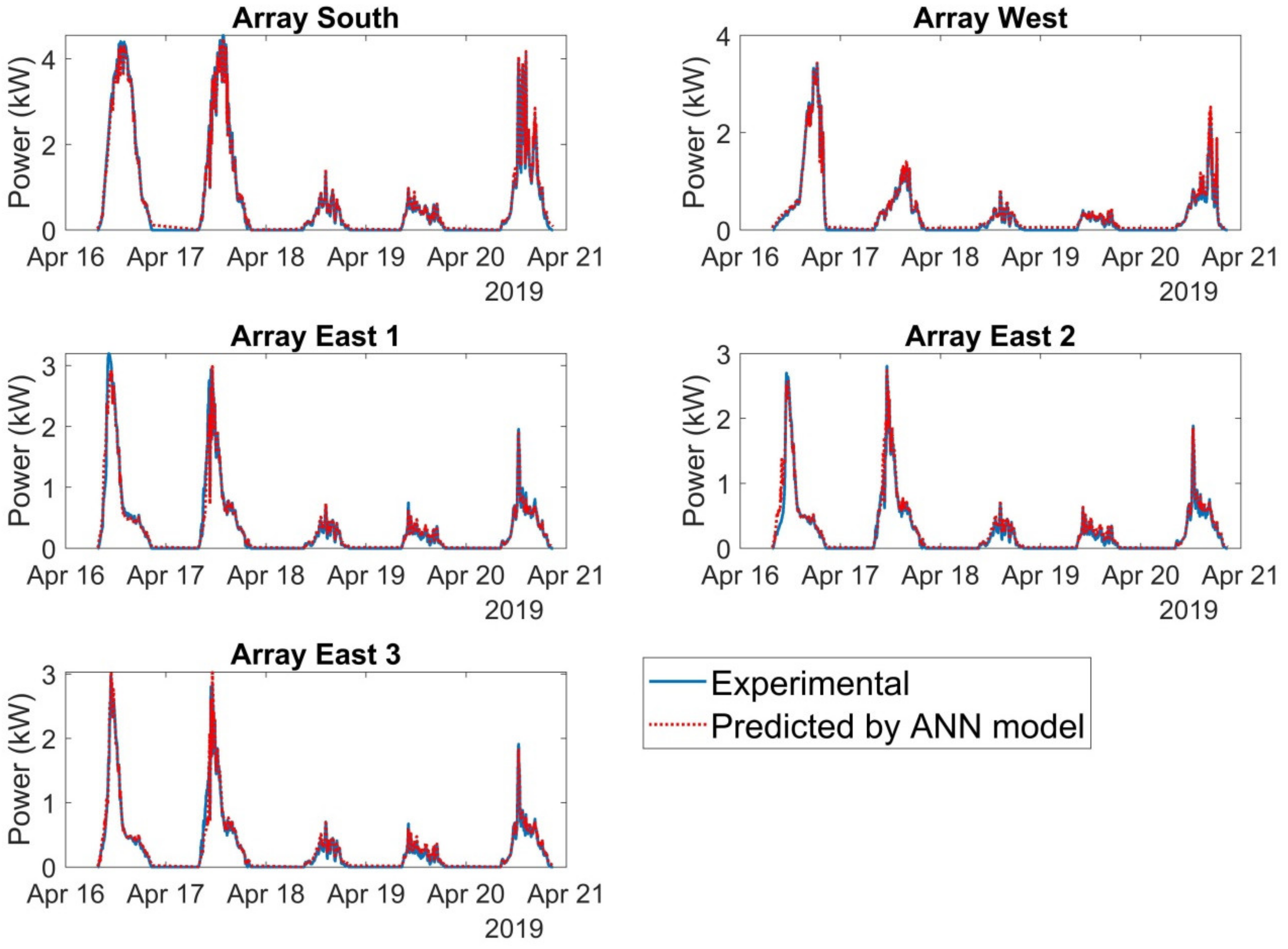
| Array | MBE (kW) | RMSE (kW) | MAE (kW) | R2 |
|---|---|---|---|---|
| South | 0.02 | 0.19 | 0.12 | 0.99 |
| West | 0.00 | 0.11 | 0.07 | 0.99 |
| East 1 | −0.01 | 0.17 | 0.07 | 0.94 |
| East 2 | 0.04 | 0.20 | 0.08 | 0.88 |
| East 3 | 0.00 | 0.21 | 0.09 | 0.89 |
Publisher’s Note: MDPI stays neutral with regard to jurisdictional claims in published maps and institutional affiliations. |
© 2022 by the authors. Licensee MDPI, Basel, Switzerland. This article is an open access article distributed under the terms and conditions of the Creative Commons Attribution (CC BY) license (https://creativecommons.org/licenses/by/4.0/).
Share and Cite
Polo, J.; Martín-Chivelet, N.; Sanz-Saiz, C. BIPV Modeling with Artificial Neural Networks: Towards a BIPV Digital Twin. Energies 2022, 15, 4173. https://doi.org/10.3390/en15114173
Polo J, Martín-Chivelet N, Sanz-Saiz C. BIPV Modeling with Artificial Neural Networks: Towards a BIPV Digital Twin. Energies. 2022; 15(11):4173. https://doi.org/10.3390/en15114173
Chicago/Turabian StylePolo, Jesús, Nuria Martín-Chivelet, and Carlos Sanz-Saiz. 2022. "BIPV Modeling with Artificial Neural Networks: Towards a BIPV Digital Twin" Energies 15, no. 11: 4173. https://doi.org/10.3390/en15114173
APA StylePolo, J., Martín-Chivelet, N., & Sanz-Saiz, C. (2022). BIPV Modeling with Artificial Neural Networks: Towards a BIPV Digital Twin. Energies, 15(11), 4173. https://doi.org/10.3390/en15114173