
Adaptive Current Control for Grid-Connected Inverter with Dynamic Recurrent Fuzzy-Neural-Network


Abstract
:1. Introduction
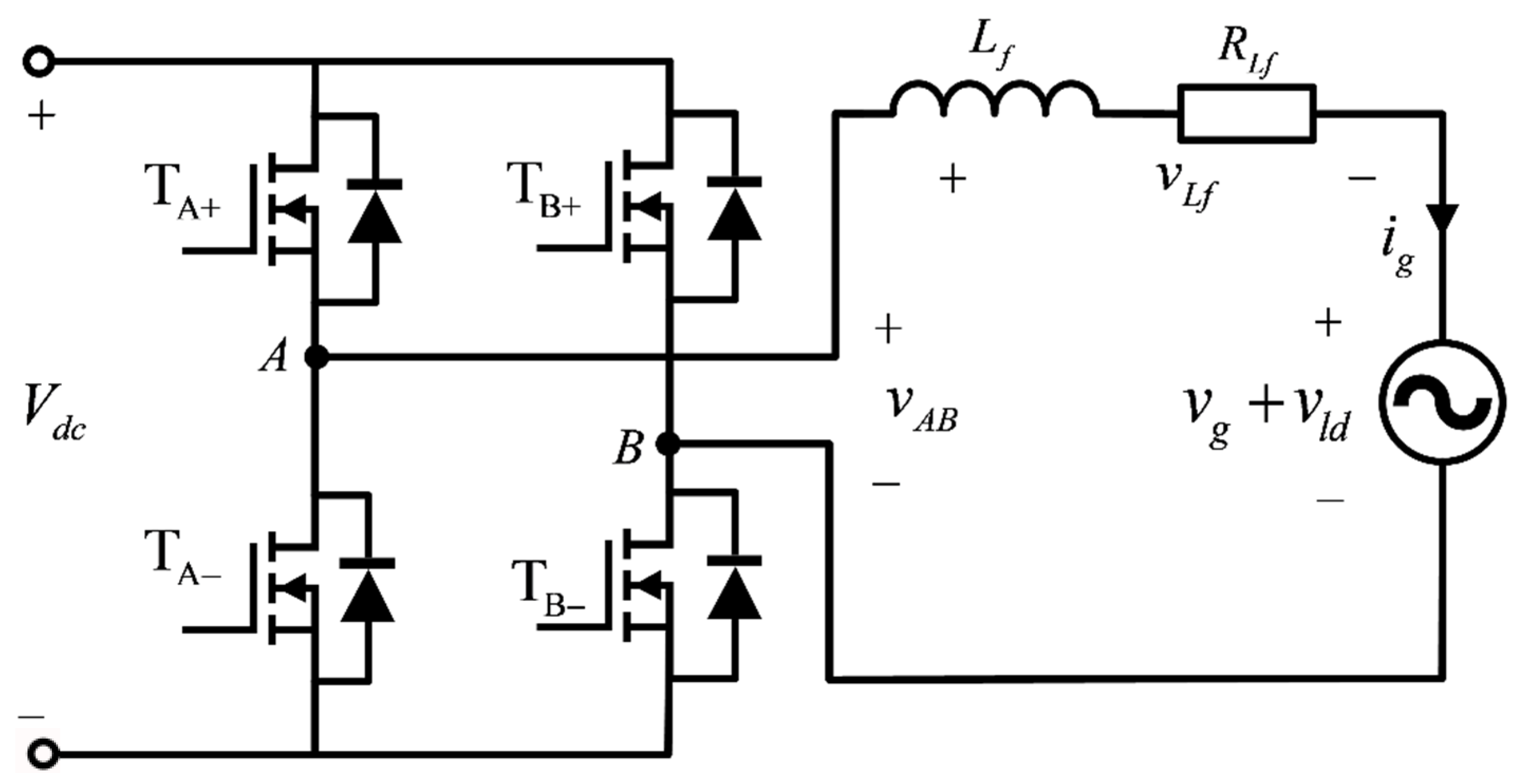
2. Descriptions of Grid-Connected Inverter
3. GISMC Design
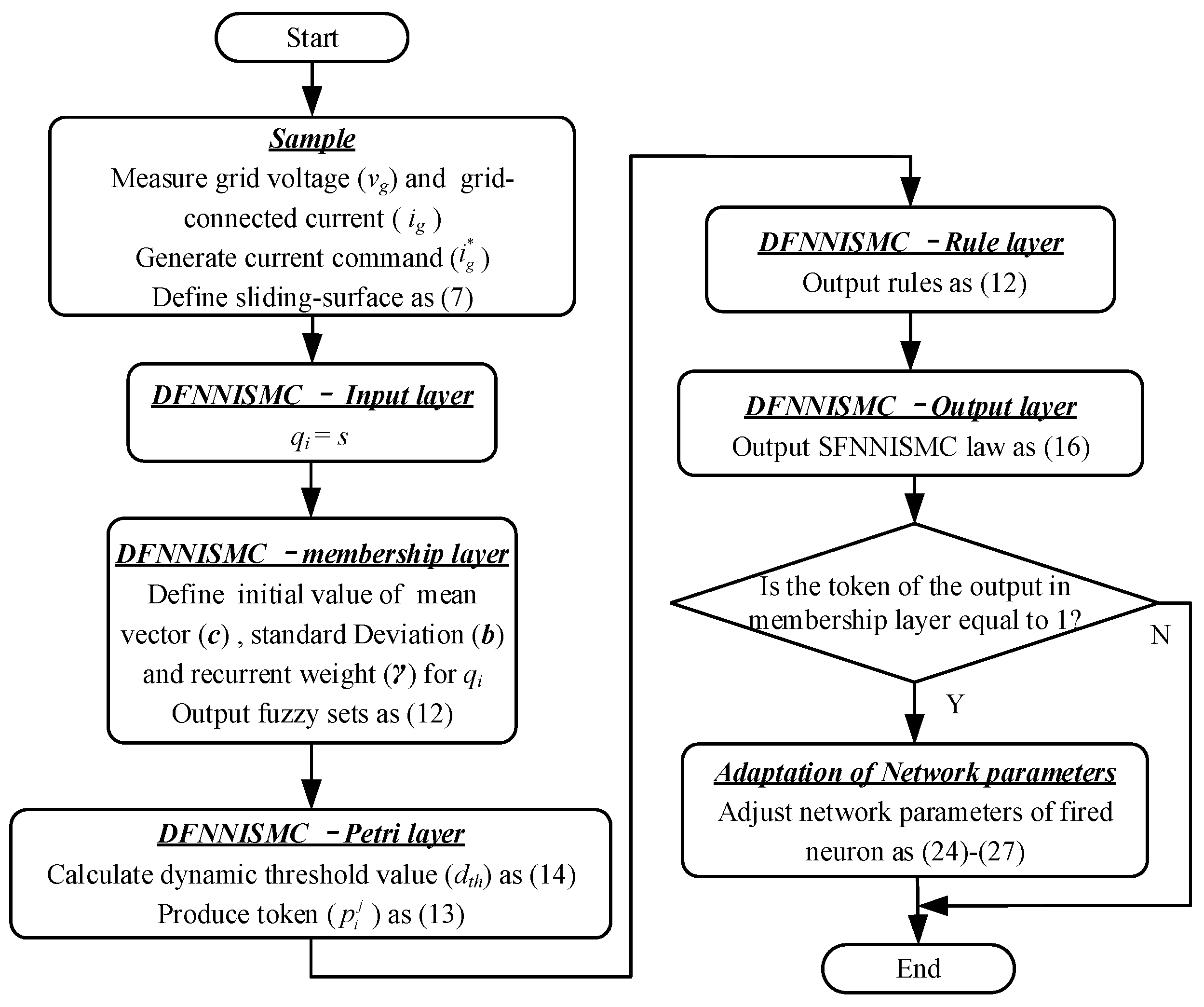
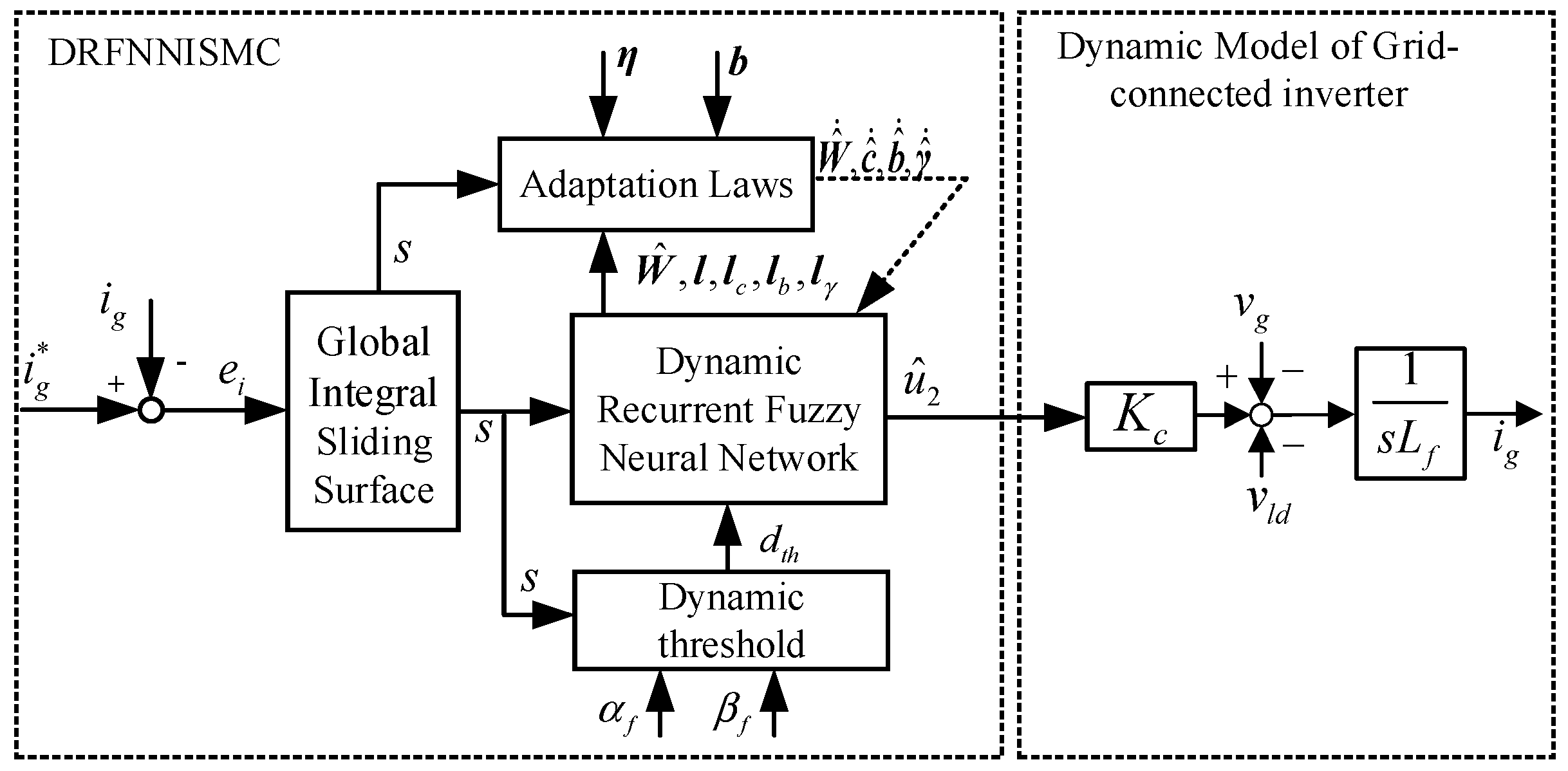
4. DRFNNISMC Design
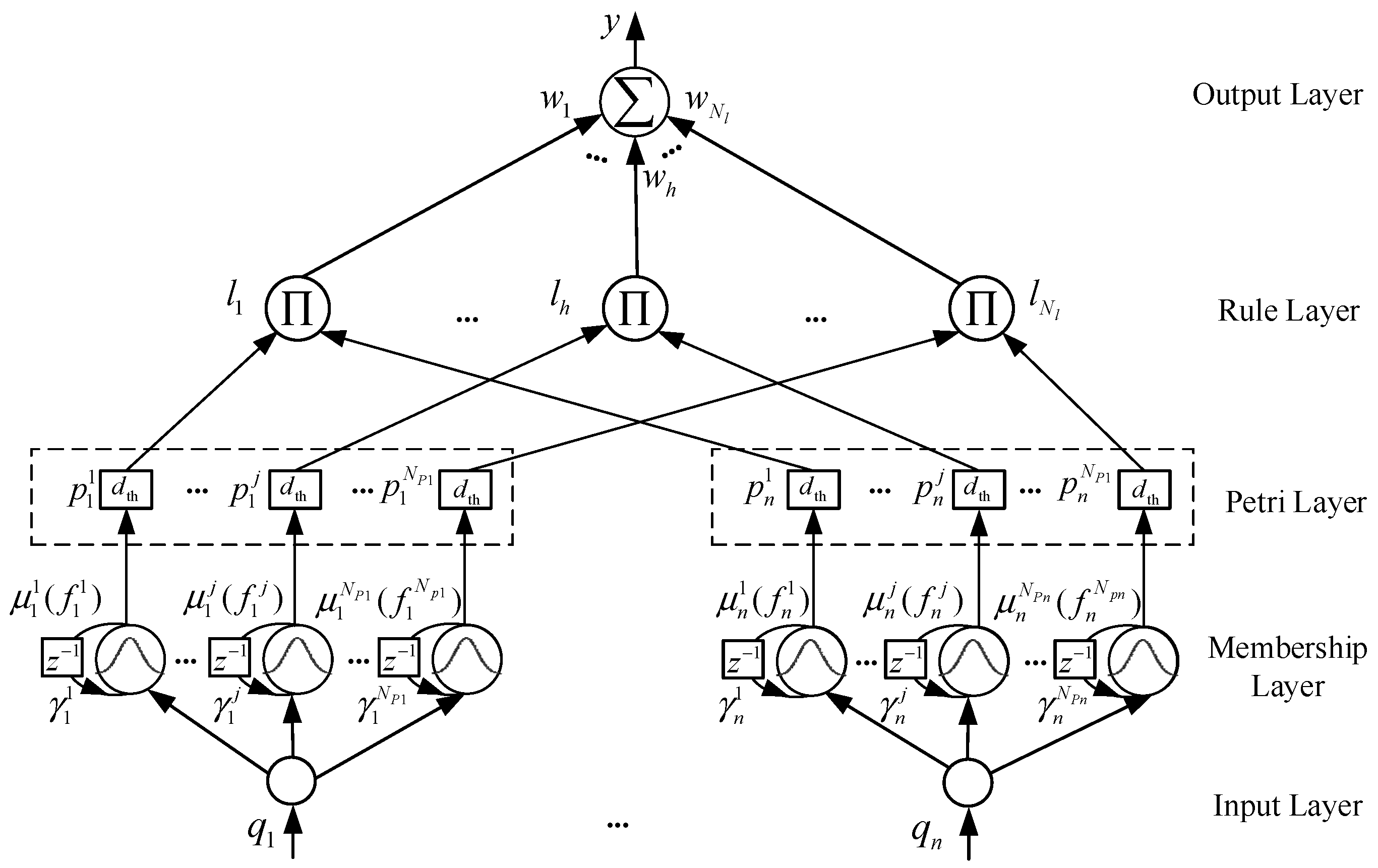
4.1. Dynamic Recurrent Fuzzy-Neural-Network
4.1.1. Input Layer
4.1.2. Gaussian Membership Layer with Recurrent Frame
4.1.3. Petri Layer
4.1.4. Layer 4 Rule Layer
4.1.5. Layer 5 Output Layer
4.2. Adaptive Scheme for Parameters of DRFNN
4.3. Stability Analysis of DRFNNISMC
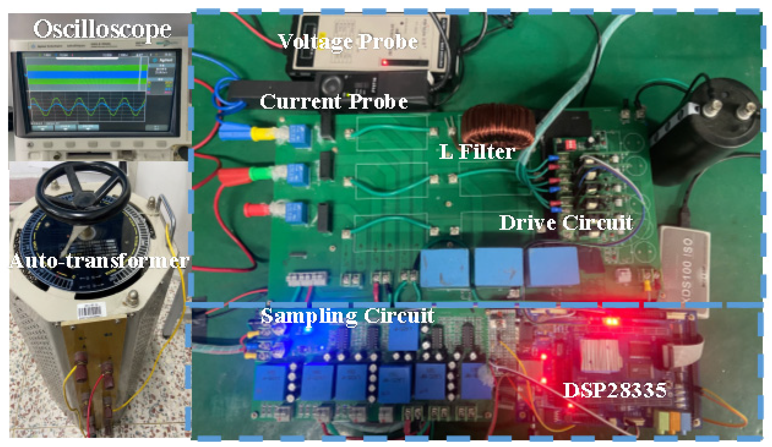
5. Experimental Verification
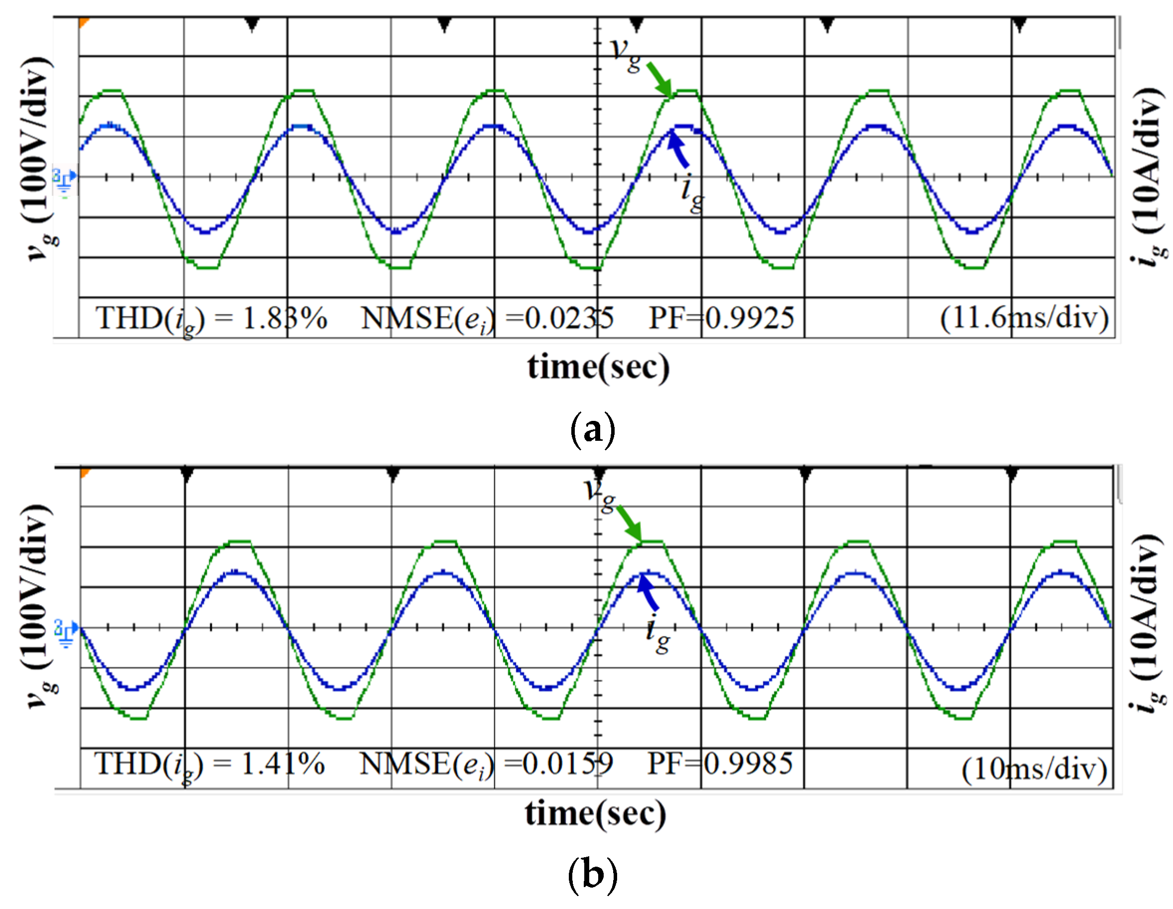
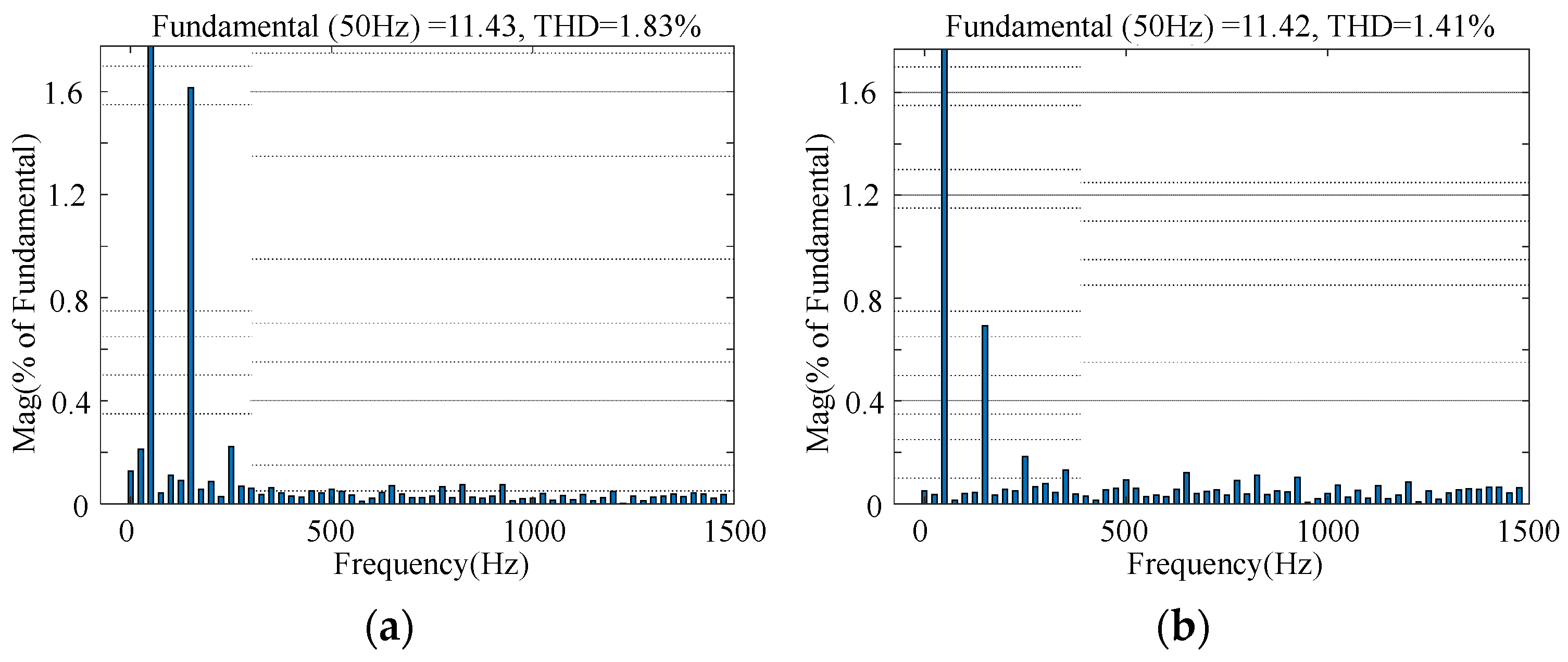
5.1. Performance Verification in Steady-State
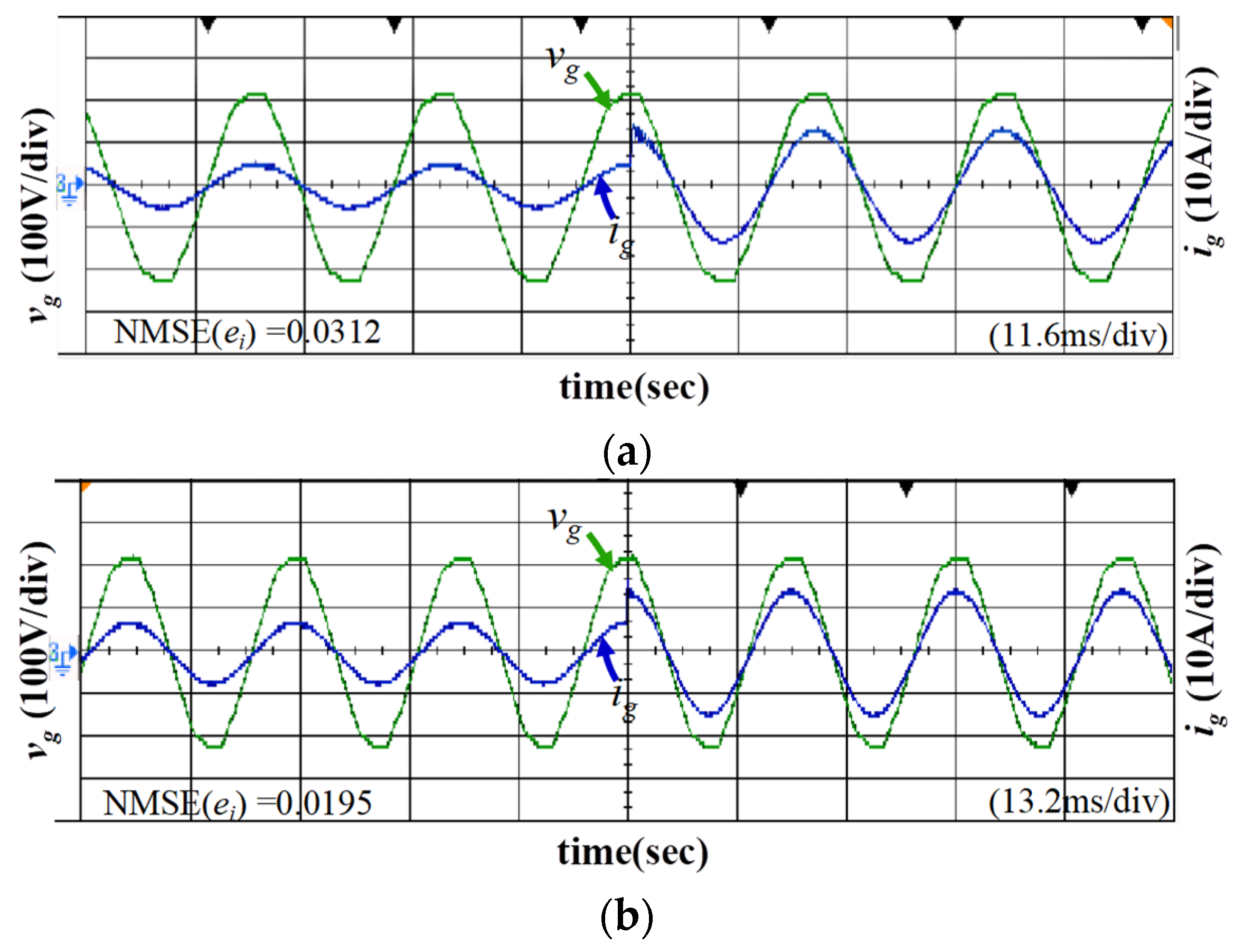
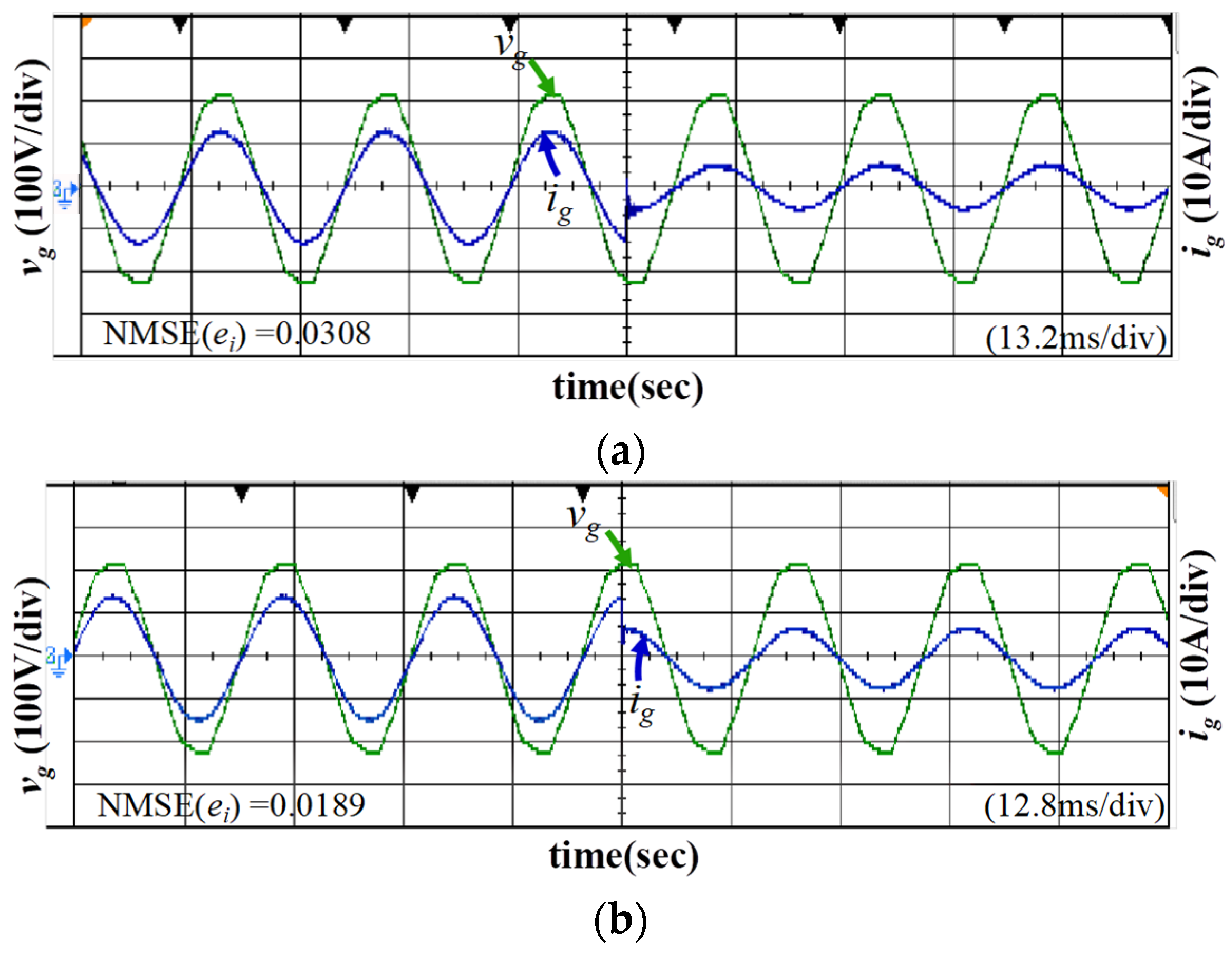
5.2. Verification of Dynamic Performance
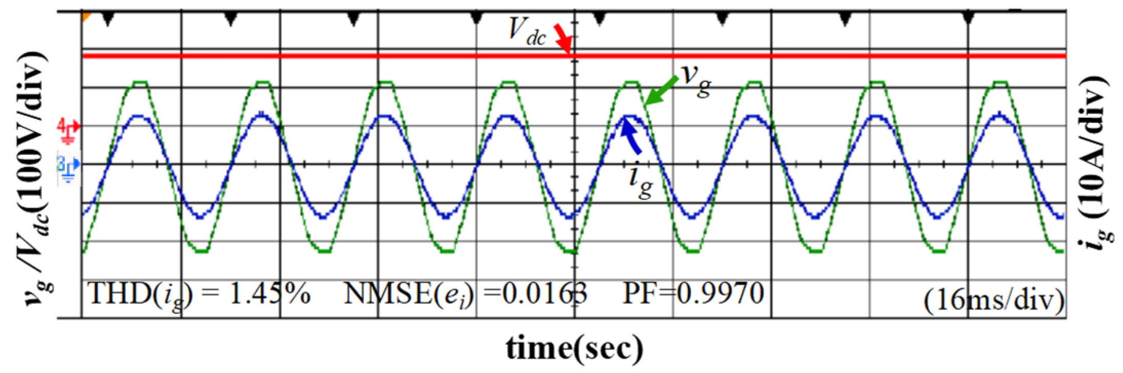
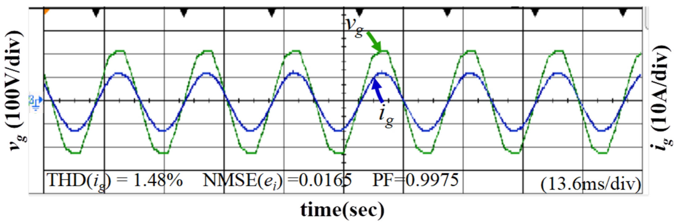
5.3. Robustness Property against Parameter Variations
5.4. Experimental Results Discussion
6. Conclusions
Author Contributions
Funding
Institutional Review Board Statement
Informed Consent Statement
Data Availability Statement
Conflicts of Interest
Abbreviations
| MG | Microgrid |
| UG | Utility grid |
| SMC | Sliding-mode control |
| GSMC | Global sliding mode control |
| GISMC | Global integral sliding-mode control |
| FNN | Fuzzy neural network |
| PN | Petri net |
| RFNN | Recurrent fuzzy neural network |
| DRFNN | Dynamic recurrent fuzzy-neural-network |
| DRFNNISMC | Dynamic recurrent fuzzy-neural-network imitating sliding-mode control |
| DC | Direct current |
| AC | Alternating current |
| KVL | Kirchhoff voltage law |
| PLL | Phase-locked loop |
| DSP | Digital signal processor |
| PWM | Pulse width modulation |
| NMSE | Normalized mean square error |
| PF | Power factor |
| THD | Total harmonic distortion |
| Variables and parameters | |
| Filter inductor | |
| Equivalent resistors of filter | |
| DC bus input voltage of inverter | |
| AC output voltage of inverter | |
| Grid-connected current | |
| Voltage of utility grid | |
| Disturbance in utility grid | |
| PWM gain of inverter | |
| Amplitude of triangular-carrier signal | |
| Modulation signal | |
| X | System state |
| u | Control input |
| f, g | Variable of state equation |
| Criterion values of state equation coefficients | |
| State equation coefficients | |
| Difference between real and criterion values of state equation coefficients | |
| System lumped uncertainty | |
| Boundary value of system lumped uncertainty | |
| Reference signal of grid-connected current | |
| Baseline model control law | |
| Current tracking error, initial value of error | |
| S | global integral sliding-surface |
| Controller parameters of GISMC | |
| u1 | Control law of GISMC |
| V1 | First Lyapunov function candidate for GISMC scheme |
| Input variables of DRFNN | |
| Recurrent weight vector in membership layer | |
| Mean deviation vector of Gaussian functions | |
| Standard deviation vector of Gaussian functions | |
| Input of jth membership neuron for the ith input signal | |
| Output of jth membership neuron for the ith input signal | |
| Npi | Number of nodes in membership layer for ith input |
| Total number of membership functions of all input signals | |
| Transition of jth membership neuron for the ith input signal | |
| dth | Dynamic threshold value |
| Parameters of dynamic threshold | |
| Output of rule layer | |
| Number of nodes in rule layer | |
| Connecting weight vector from rule layer to output layer | |
| y | Output of DRFNN |
| Difference between optimal and estimated vector | |
| Optimal DRNNISMC law | |
| Minimum mapping error vector | |
| Approximation error | |
| Coefficient vectors of first-order terms in Taylor series | |
| Summation of higher-order term in Taylor series | |
| H | Uncertain term in approximation error |
| V2 | Second Lyapunov function candidate for DRFNNISMC scheme |
| G | Defined function for proof of stability and convergence of DRFNNISMC system |
Appendix A
References
- Muhtadi, A.; Pandit, D.; Nguyen, N.; Mitra, J. Distributed Energy Resources Based Microgrid: Review of Architecture, Control, and Reliability. IEEE Trans. Ind. Appl. 2021, 57, 2223–2235. [Google Scholar] [CrossRef]
- Bihari, S.P.; Sadhu, P.K.; Sarita, K.; Khan, B.; Arya, L.D.; Saket, R.K.; Kothari, D.P. A Comprehensive Review of Microgrid Control Mechanism and Impact Assessment for Hybrid Renewable Energy Integration. IEEE Access 2021, 9, 88942–88958. [Google Scholar] [CrossRef]
- Wu, D.; Tang, F.; Dragicevic, T.; Vasquez, J.C.; Guerrero, J.M. A control architecture to coordinate renewable energy sources and energy storage systems in islanded microgrids. IEEE Trans. Smart Grid 2015, 6, 1156–1166. [Google Scholar] [CrossRef] [Green Version]
- Kakran, S.; Chanana, S. Smart operations of smart grids integrated with distributed generation: A review. Renew. Sustain. Energy Rev. 2018, 81, 524–535. [Google Scholar] [CrossRef]
- Chen, X.; Ruan, X.; Yang, D.; Zhao, W.; Jia, L. Injected grid current quality improvement for a voltage-controlled grid-connected inverter. IEEE Trans. Power Electron. 2017, 33, 1247–1258. [Google Scholar] [CrossRef]
- Kumar, N.; Saha, T.K.; Dey, J. Sliding-mode control of PWM dual inverter-based grid-connected PV system: Modeling and performance analysis. IEEE J. Emerg. Sel. Top. Power Electron. 2016, 4, 435–444. [Google Scholar] [CrossRef]
- Dhar, S.; Dash, P.K. A new backstepping finite time sliding mode control of grid connected PV system using multivariable dynamic VSC model. Int. J. Electr. Power Energy Syst. 2016, 82, 314–330. [Google Scholar] [CrossRef]
- Alquthami, T.; Zulfiqar, M.; Kamran, M.; Milyani, A.H.; Rasheed, M.B. A Performance Comparison of Machine Learning Algorithms for Load Forecasting in Smart Grid. IEEE Access 2022, 10, 48419–48433. [Google Scholar] [CrossRef]
- Xiao, D.L.; Chen, H.Y.; Wei, C.; Bai, X.Q. Statistical Measure for Risk-Seeking Stochastic Wind Power Offering Strategies in Electricity Markets. J. Mod. Power Syst. Clean Energy 2021, 1–6. [Google Scholar] [CrossRef]
- Zeb, K.; Nazir, M.; Ahmad, I.; Uddin, W.; Kim, H.-J. Control of Transformerless Inverter-Based Two-Stage Grid-Connected Photovoltaic System Using Adaptive-PI and Adaptive Sliding Mode Controllers. Energies 2021, 14, 2546. [Google Scholar] [CrossRef]
- Chen, S.; Lai, Y.M.; Tan, S.C.; Tse, C.K. Fast response low harmonic distortion control scheme for voltage source inverters. IET Power Electron. 2009, 2, 574–584. [Google Scholar] [CrossRef]
- Chu, Y.; Fei, J.; Hou, S. Dynamic Global Proportional Integral Derivative Sliding Mode Control Using Radial Basis Function Neural Compensator for Three-Phase Active Power Filter. Trans. Inst. Meas. Control 2018, 40, 3549–3559. [Google Scholar] [CrossRef]
- Wai, R.J.; Lin, C.Y.; Huang, Y.C.; Chang, Y.R. Design of high-performance stand-alone and grid-connected inverter for distributed generation applications. IEEE Trans. Ind. Electron. 2013, 60, 1542–1555. [Google Scholar] [CrossRef]
- Wang, H.; Li, Z.; Jin, X.; Huang, Y.; Kong, H.; Yu, M.; Ping, Z.; Sun, Z. Adaptive Integral Terminal Sliding Mode Control for Automobile Electronic Throttle via an Uncertainty Observer and Experimental Validation. IEEE Trans. Veh. Technol. 2018, 67, 8129–8143. [Google Scholar] [CrossRef]
- Shi, P.; Liu, M.; Zhang, L. Fault-Tolerant Sliding-Mode-Observer Synthesis of Markovian Jump Systems Using Quantized Measurements. IEEE Trans. Ind. Electron. 2015, 62, 5910–5918. [Google Scholar] [CrossRef] [Green Version]
- Shadoul, M.; Yousef, H.; Abri, R.; Al-Hinai, A. Adaptive Fuzzy Approximation Control of PV Grid-Connected Inverters. Energies 2021, 14, 942. [Google Scholar] [CrossRef]
- Livinti, P. Comparative Study of a Photovoltaic System Connected to a Three-Phase Grid by Using PI or Fuzzy Logic Controllers. Sustainability 2021, 13, 2562. [Google Scholar] [CrossRef]
- Haq, I.U.; Khan, Q.; Khan, I.; Akmeliawati, R.; Nisar, K.S.; Khan, I. Maximum power extraction strategy for variable speed wind turbine system via neuro-adaptive generalized global sliding mode controller. IEEE Access 2020, 8, 128536–128547. [Google Scholar] [CrossRef]
- Zhu, Y.; Fei, J. Adaptive Global Fast Terminal Sliding Mode Control of Grid-connected Photovoltaic System Using Fuzzy Neural Network Approach. IEEE Access 2017, 5, 9476–9484. [Google Scholar] [CrossRef]
- Chu, Y.; Fei, J.; Hou, S. Adaptive global sliding-mode control for dynamic systems using double hidden layer recurrent neural network structure. IEEE Trans Neural Netw. Learn. Syst. 2020, 31, 1297–1309. [Google Scholar] [CrossRef]
- Wai, R.; Lin, Y.; Liu, Y. Design of Adaptive Fuzzy-Neural-Network Control for a Single-Stage Boost Inverter. IEEE Trans. Power Electron. 2015, 30, 7282–7298. [Google Scholar] [CrossRef]
- Yang, Y.; Wai, R.J. Design of adaptive fuzzy-neural-network-imitating sliding-mode control for parallel-inverter system in islanded micro-grid. IEEE Access 2021, 9, 56376–56396. [Google Scholar] [CrossRef]
- Wai, R.J.; Muthusamy, R. Design of Fuzzy-Neural-Network-Inherited Backstepping Control for Robot Manipulator Including Actuator Dynamics. IEEE Trans. Fuzzy Syst. 2014, 22, 709–722. [Google Scholar] [CrossRef]
- Wai, R.; Yao, J.; Lee, J. Backstepping Fuzzy-Neural-Network Control Design for Hybrid Maglev Transportation System. IEEE Trans. Neural Netw. Learn. Syst. 2015, 26, 302–317. [Google Scholar]
- Wai, R.J.; Liu, C.M. Design of Dynamic Petri Recurrent Fuzzy Neural Network and Its Application to Path-Tracking Control of Nonholonomic Mobile Robot. IEEE Trans. Ind. Electron. 2009, 56, 2667–2683. [Google Scholar]
- El-Sousy, F.F.M.; Abuhasel, K.A. Adaptive Nonlinear Disturbance Observer Using a Double-Loop Self-Organizing Recurrent Wavelet Neural Network for a Two-Axis Motion Control System. IEEE Trans. Ind. Appl. 2018, 54, 764–786. [Google Scholar] [CrossRef]
- Liu, S.; Guo, X.; Zhang, L. Robust Adaptive Backstepping Sliding Mode Control for Six-Phase Permanent Magnet Synchronous Motor Using Recurrent Wavelet Fuzzy Neural Network. IEEE Access 2017, 5, 14502–14515. [Google Scholar]
- Chen, F.; Fei, J.; Xue, Y. Double Recurrent Perturbation Fuzzy Neural Network Fractional-Order Sliding Mode Control of Micro Gyroscope. IEEE Access 2021, 9, 55352–55363. [Google Scholar] [CrossRef]
- Fei, J.; Liu, L. Real-Time Nonlinear Model Predictive Control of Active Power Filter Using Self-Feedback Recurrent Fuzzy Neural Network Estimator. IEEE Trans. Ind. Electron. 2022, 69, 8366–8376. [Google Scholar] [CrossRef]
- Tan, K.H.; Tseng, T.Y. Seamless Switching and Grid Reconnection of Microgrid Using Petri Recurrent Wavelet Fuzzy Neural Network. IEEE Trans. Power Electron. 2021, 36, 11847–11861. [Google Scholar] [CrossRef]
- Lin, F.J.; Chen, S.G.; Hsu, C.W. Intelligent backstepping control using recurrent feature selection fuzzy neural network for synchronous reluctance motor position servo drive system. IEEE Trans. Fuzzy Syst. 2019, 27, 413–427. [Google Scholar] [CrossRef]
- Hou, S.; Chu, Y.; Fei, J. Intelligent global sliding mode control using recurrent feature selection neural network for active power filter. IEEE Trans. Ind. Electron. 2021, 68, 7320–7329. [Google Scholar] [CrossRef]
- Li, Y.; Mai, R.; Lu, L.; He, Z. Active and reactive currents decomposition-based control of angle and magnitude of current for a parallel multi-inverter IPT system. IEEE Trans. Power Electron. 2017, 32, 1602–1614. [Google Scholar] [CrossRef]
- Astrom, K.J.; Wittenmark, B. Adaptive Control; Addison-Wesley: New York, NY, USA, 1995. [Google Scholar]
- Wang, L.X. A Course in Fuzzy Systems and Control; Prentice-Hall: Englewood Cliffs, NJ, USA, 1997. [Google Scholar]


| Circuit Parameters | Value |
|---|---|
| DC bus voltage | 200 V |
| Current command (RMS) | 10 A |
| Grid voltage (RMS) | 110 V |
| Filter inductance | 2 mH |
| Fundamental frequency | 50 Hz |
| Switching frequency | 15 kHz |
| Performance Control Methods | GISMC | Proposed DRFNNISMC | |
|---|---|---|---|
| Output power 1 kW | THD (ig) | 1.83% | 1.41% |
| PF | 0.9925 | 0.9985 | |
| NMSE (ei) | 0.0235 | 0.0159 | |
| Power variations from 0.5 kW to 1 kW | NMSE (ei) | 0.0312 | 0.0195 |
| Power variations from 1 kW to 0.5 kW | NMSE (ei) | 0.0308 | 0.0189 |
| DC-bus voltage fluctuation (Vdc = 180 V) | THD (ig) | / | 1.45% |
| PF | / | 0.9970 | |
| NMSE (ei) | / | 0.0163 | |
| Inductance variation (Lf = 1.5 mH) | THD (ig) | / | 1.48% |
| PF | / | 0.0165 | |
| NMSE (ei) | / | 0.9975 | |
| Dependence on system parameters | High | None | |
| Robustness | Good | Favorable | |
| Chattering | Chattering | None | |
| Learning ability | None | Online self-learning | |
Publisher’s Note: MDPI stays neutral with regard to jurisdictional claims in published maps and institutional affiliations. |
© 2022 by the authors. Licensee MDPI, Basel, Switzerland. This article is an open access article distributed under the terms and conditions of the Creative Commons Attribution (CC BY) license (https://creativecommons.org/licenses/by/4.0/).
Share and Cite
Wang, Y.; Yang, Y.; Liang, R.; Geng, T.; Zhang, W. Adaptive Current Control for Grid-Connected Inverter with Dynamic Recurrent Fuzzy-Neural-Network. Energies 2022, 15, 4163. https://doi.org/10.3390/en15114163
Wang Y, Yang Y, Liang R, Geng T, Zhang W. Adaptive Current Control for Grid-Connected Inverter with Dynamic Recurrent Fuzzy-Neural-Network. Energies. 2022; 15(11):4163. https://doi.org/10.3390/en15114163
Chicago/Turabian StyleWang, Yeqin, Yan Yang, Rui Liang, Tao Geng, and Weixing Zhang. 2022. "Adaptive Current Control for Grid-Connected Inverter with Dynamic Recurrent Fuzzy-Neural-Network" Energies 15, no. 11: 4163. https://doi.org/10.3390/en15114163
APA StyleWang, Y., Yang, Y., Liang, R., Geng, T., & Zhang, W. (2022). Adaptive Current Control for Grid-Connected Inverter with Dynamic Recurrent Fuzzy-Neural-Network. Energies, 15(11), 4163. https://doi.org/10.3390/en15114163