Distributed Weight Adaptive Control for Frequency Regulation of Islanded Microgrid

Abstract

The consensus control method based on a multi-agent system has been widely applied in the distributed control and optimization of microgrids. However, the following drawbacks are still common in current research: (1) ignoring the influence of consensus control commands on the synchronization stability of the physical grid under primary control; (2) only focusing on improving one property ofcontrol performance, lacking comprehensive considerations of multiple properties. With the aim of solving these problems, in this paper we propose a weight-adaptive robust control strategy for implementing distributed frequency regulation of islanded microgrids. Firstly, the frequency synchronization stability of the physical layer is analyzed by means of a coupled oscillator theory and the design objectives of the controllable parameters for the information layer are formed. Subsequently, the relationship between the weight coefficients and the two important control performances of convergence speed and delay robustness is strictly analyzed. Based on this, an adaptive coefficient that can be autonomously adjusted according to the frequency deviation is designed to achieve a trade-off between convergence speed and delay robustness. Finally, three simulation studies are presented to verify the effectiveness of the proposed control strategy.

1. Introduction

Microgrids, which are small autonomous power distribution systems, have significantly improved the reliability and quality of power supply performance in built environments [1], industrial zones [2], and large facilities [3]. They can operate in islanded or grid-connected modes [4,5,6]. In islanded mode, the microgrid needs to independently face the intermittent and random disturbances caused by distributed generators (DGs) in the absence of a large external power grid [7], which means that the frequency stability of islanded microgrids faces severe challenges. In early research, centralized control was widely used to achieve frequency regulation [8,9,10]. Despite the simple control structure used, the drawbacks of this control method are quite manifest. (1) A single-point failure of the microgrid central controller will cause a breakdown of the entire system. (2) The rigid structure of centralized control reduces the flexibility, scalability, and reliability of the microgrid.

Alternatively, distributed control, especially the consensus control method based on multi-agent systems (MAS), has become a research hotspot due to the need for matching with the control requirements of microgrids. At present, the consensus control method is generally usedto solve problems such as frequency/voltage regulation, power sharing, economic dispatching, and state of charge (SoC) balancing. In [11], the secondary voltage regulation target was transformed into a synchronization problem, which was solved by means of a feedback linearization method. The same method was used in [12] to achieve secondary frequency support of microgrids based on sparse communication lines. In [13], a distributed average control method was proposed, implementing secondary regulation and power-sharing based only on local and neighbor information. The economic dispatching problem was studied in [14], in which the convex optimization objective was implemented via a first-order discrete consensus approach, through setting the incremental cost of each DG as the consensus variable. In [15], a nonlinear sliding mode control method was proposed for implementing SoC balancing among storage devices in a DC microgrid.

Other studies, presented in [16,17,18,19,20,21,22,23,24,25], have focused on enhancing the control performance of consensus methods. In terms of convergence speed, a distributed diffusion strategy was proposed in [16] for implementing microgrid optimization, which accelerated the convergence process by adding a random gradient term. In [17,18], an improvement in the convergence speed was achieved via the optimization design of weight coefficients in feedback linearization control. A finite time control protocol with accelerated convergence and disturbance attenuation capabilities was used in [19,20] to achieve frequency and voltage restoration in an islanded microgrid. Compared with the convergence speed, less research has been conducted on delay robustness. In [21], the upper bounds of the communication delay time in distributed economic dispatch control were strictly analyzed using the Nyquist criterion. In [22], the influence of communication delays on the secondary control of microgrids was considered, and the sensitivity of time delays was fully investigated using small-signal stability theory. In addition, other measures of control performance, such as the robustness of uncertain topologies [23], global cooperation without leaders [24], robustness under the influence of noise [25], etc., have gradually been taken seriously in recent years. However, an outstanding problem of the above studies is the fact that they only focus on improving one type of control performance and lack comprehensive considerations of multiple properties. Generally, there is a potential conflict between different measures of control performance; for example, only stressing the convergence speed may result in poor delay robustness.

Another problem which needs to be addressed is the synchronization stability of the physical layer. The microgrid under consensus control is a two-layer coupled network, including the information layer formed by the communication network and the physical layer formed by the transmission lines (as shown in Figure 1). As the upper-layer control, the commands generated by the consensus control will inevitably change the operating characteristics of the physical layer under primary control. Therefore, the synchronization and the stability of the microgrid can be degraded or even destroyed if the commands are not appropriate. Unfortunately, the current studies all focus on the design of control strategies at the information layer [16,17,18,19,20,21,22,23,24,25], lacking a rigorous analysis of the stable operating conditions of the physical power grid.

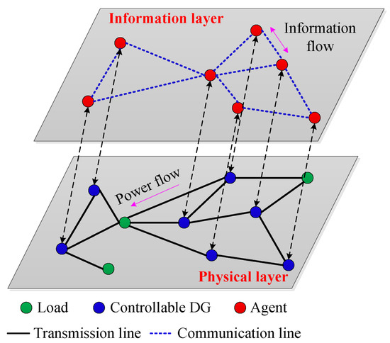
Figure 1. The two-layer model of an islanded microgrid.

Motivated by the above problems, here we investigate a distributed frequency regulation method for islanded microgrids, and achieve three main contributions as follows. (1) We extend the Kuramoto theory proposed in [26] to the frequency regulation of microgrids, and the frequency synchronization stability of the physical layer under primary control is analyzed, thereby forming the control objectives of the information layer. The consensus control method designed based on these objectives does not alter the stability of the physical layer under primary control. (2) Two control performances, convergence speed and delay robustness, are considered comprehensively, and their relationship with the weight coefficients is strictly analyzed. (3) A weight-adaptive robust control strategy is proposed, which dynamically adjusts the weight coefficients based on frequency deviations. Therefore, not only is the fast convergence capability of the traditional feedback linearization control inherited, but the delay robustness is also significantly improved.

The rest of this paper is organized as follows. Section 2 discusses the synchronization stability of the microgrid frequency in the physical layer. A weight-adaptive robust control strategy is proposed in Section 3 to implement secondary frequency regulation. Three simulation cases are designed in Section 4 to verify control performances. Section 5 presents the conclusions of this paper.

2. Synchronization Stability Analysis of the Physical Layer

In this section, we analyze the basic conditions for the synchronization stability of the physical layer, which will guide the design of the consensus control system at the information layer.

2.1. Two-Layer Control Structure

A two-layer control structure for islanded microgrids is depicted in Figure 1, where the bottom layer is the physical system consisting of DGs and loads. DGs can be divided into non-dispatchable DGs (such as small diesel generators) that provide the generation of renewable energy, and bidirectionally controllable DGs (such as controllable wind turbines, photovoltaics, etc.) that can store and provide energy. Since our focus is on coordinated control at the system level, the specific properties of each type of DG are not investigated here. As in the studies in [8,9,10,11,12,13,14,15,16,17,18,19,20,21,22], all DGs are designated as controllable DGs in this paper. The top layer is the information system, constructed by agents. Each controllable DG corresponds to an agent. In the physical layer, natural coupling is formed through the transmission lines. Furthermore, in the information layer, auxiliary coupling is constructed by sparse communication lines.

2.2. Graph Theory

The networks of the physical layer and information layer can be regarded as two weighted graphs. We define a graph G = (V,E,A), where V = {1,2, …, n} represents the set of nodes, E⊆V×V represents the set of edges, and A = [a${}_{ij}$]${}_{n\times n}$ represents the n-dimensional adjacency matrix. For a${}_{ij}$, if (i,j)$\in$E, then a${}_{ij}$ = 0; otherwise a${}_{ij}$$>$0 and satisfies a${}_{ij}$ = a${}_{ji}$. Let N${}_i$ = {j ∈ V: (j,i) ∈ E} represent the set of neighbors of node i and define the matrix D = diag{d${}_i$}, where d${}_i$ = ∑${}_{j\in N_i}$a${}_{ij}$. Then, the Laplacian matrix satisfies L = D−A, which is a semi-definite matrix.

2.3. Physical Layer Model

The physical layer consists of DGs, loads, and transmission lines, among which the loads and transmission lines, as passive nodes, do not affect the synchronization stability of the system frequency [27]. In fact, through Kron reduction, the microgrid can be equivalently transformed into a system where only controllable DGs are interconnected (the detailed simplification process can be found in [28,29]. We do not describe this in detail in this paper). Therefore, we only need to focus our analysis on DG. The DG is connected to the AC microgrid with the inverter as the interface. The primary control of the i-th inverter is as follows [27].

$$\left\{\begin{array}{c}{\dot{\theta }}_i={\omega }_i-{\omega }_0\hfill \\ P_i=P_i^{*}-K_i{\dot{\theta }}_i\hfill \end{array}\right.$$

(1)

where $\theta$ and $\omega$ are the phase angle and the angular frequency, respectively. ${\omega }_0$ is the nominal system frequency. K is the frequency droop coefficient. P and P${}^{*}$ are the measured and the nominal active power, respectively, where P${}^{*}$ is updated through the control of the information layer.

According to the power flow relationship, the output active power of inverter-i can be written as follows [30,31].

$$P_i=\sum _{i,j\in V_p,j\in N_{pi}}{V}_i{V}_j{y}_{ij}sin({\theta }_i-{\theta }_j)$$

(2)

where V${}_p$ represents the set of controllable DGs. N${}_{pi}$ represents the set of neighbor DGs of DGi. V is the AC voltage. y${}_{ij}$ is the absolute value of the admittance of line (i, j).

Then, the unified model of DGs can be described as

$$K_i{\dot{\theta }}_i=P_i^{*}-\sum _{i,j\in V_p,j\in N_{pi}}{V}_i{V}_j{y}_{ij}sin({\theta }_i-{\theta }_j)$$

(3)

which is equivalent to

$${\dot{\theta }}_i=\frac{P_i^{*}}{K_i}-\sum _{i,j\in V_p,j\in N_{pi}}\frac{V_i{V}_j{y}_{ij}}{K_i}sin({\theta }_i-{\theta }_j)$$

(4)

2.4. Synchronization Stability Analysis

As a classical phase-coupled oscillator model, the Kuramoto model has been widely investigated in mathematics and physics. Its generalized form can be written as

$${\dot{\xi }}_i={\mathsf{\Omega }}_i-\sum _{i=1}^n{a}_{ij}sin({\xi }_i-{\xi }_j)$$

(5)

where $\xi$${}_i$ is the phase of oscillator i. $\mathsf{\Omega }$${}_i$ is the natural frequency of oscillator i. n is the number of oscillators. a${}_{ij}$ is the coupling strength between oscillator i and oscillator j.

Comparing (4) and (5), we can observe that they are very similar in structure. This similarity was discovered by John W.S.P. et al in [27]. They rigorously demonstrated the equivalence between the microgrid physical layer model and the Kuramoto model in [24] (see Lemma 1 in [27]). Their research results provide support for the application of the Kuramoto coupled oscillator theory in microgrids.

The authors in [26] studied the stability domain of the Kuramoto model and their results are shown in Lemma 1.

Lemma 1.

([26]) The Kuramoto model with fixed topology satisfies

$$D(\delta (t))\le D(\delta (0))e^{-CcosD(\xi (0)t)}$$

(6)

if

$$0<D(\xi (0))<\pi ,C>\frac{D(\mathsf{\Omega })}{sinD(\xi (0))}$$

(7)

where D(x) = max{x${}_i$− x${}_j$}(i,j= 1,2,…,n. x represents $\xi$, $\delta$, or $\mathsf{\Omega }$). $\delta$ is the angular frequency of the oscillator, $\delta$${}_i$ = $\dot{\xi }$${}_i$. Both 0 and t in parentheses represent time. C is a constant that satisfies

$$C=\underset{i\ne j}{min}\{a_{ij}+a_{ji}+\sum _{k\ne i,j}min\{a_{ik},a_{jk}\}\}$$

(8)

On the basis of [26,27], by constructing the mapping relationship shown in Table 1, we can obtain the basic conditions for the synchronization stability of the physical layer under primary control.

$$\left\{\begin{array}{c}0<\underset{i,j\in V_p}{max}|{\theta }_i(0)-{\theta }_j(0)|<\pi \hfill \\ C>\frac{\underset{i,j\in V_p}{max}|\frac{P_i^{*}}{K_i}-\frac{P_j^{*}}{K_j}|}{sin(\underset{i,j\in V_p}{max}|{\theta }_i(0)-{\theta }_j(0)|)}\hfill \\ C=\underset{i\ne j}{min}\{\frac{V_i{V}_j{y}_{ij}}{K_i}+\frac{V_j{V}_i{y}_{ji}}{K_j}+\sum _{l\in V_p,k\ne i,j}min\{\frac{V_i{V}_k{y}_{ik}}{K_i},\frac{V_j{V}_k{y}_{jk}}{K_j}\}\}\hfill \end{array}\right.$$

(9)

Table 1. Correspondence between the parameters of the physical layer microgrid model and the Kuramoto model.

Kuramoto	Physical Layer
$\xi$${}_i$	$\theta$${}_i$
$\delta$${}_i$	$\omega$${}_i$
$\mathsf{\Omega }$${}_i$	P${}_i^{*}$/K${}_i$
a${}_{ij}$	V${}_i$V${}_j$y${}_{ij}$/K${}_i$

From Lemma 1, we know that when t→∞, the maximum frequency deviation tends to 0, and the synchronization stability of the physical layer is achieved. Since the consensus control of the information layer will change the controllable parameters of the physical layer, it becomes necessary to analyze the relationship between the parameters and the stability conditions.

In (9), the parameters P${}_i^{*}$, K${}_i$, V${}_{i/j}$, y${}_{ij}$, and $\theta$${}_{i/j}$ can affect the stability of physical layer frequency, where V${}_{i/j}$, y${}_{ij}$, and $\theta$${}_{i/j}$ cannot be changed by the consensus control due to their direct correlation with the microgrid’s physical structure. Therefore, we only need to analyze the controllable parameters P${}_i^{*}$ and K${}_i$.

Without the loss of generality, the droop coefficient can be designed as follows [19].

$$K_i=\frac{P_i^{*}}{{\omega }_i^{\max }-{\omega }_0}$$

(10)

where $\omega$${}^{max}$ is the upper limit of angular frequency. In an AC microgrid, the upper limit of each DG is the same, i.e., $\omega$${}_i^{\max }$ = $\omega$${}^{\max }$ (i = 1,…,n).

Bringing (10) into (9), we can prove that C > $\mid P_i^{*}/K_i-P_j^{*}/K_j\mid$ = 0 always holds under droop control. This indicates that the physical layer under primary control is sufficient to achieve frequency exponential convergence, and the stabilized synchronization solution is a common value as follows.

$${\omega }_{syn}=\frac{\sum P_i^{*}-\sum P_i^l}{\sum K_i}+{\omega }_0$$

(11)

Since the consensus control of the information layer may update P${}^{*}$, its changes are discussed next. When the droop coefficient is constant, the change in P${}^{*}$ is equivalent to the translation of the droop characteristic curve, as shown in Figure 2, where two DGs are defined to represent a microgrid (blue lines corresponds to DG1 and red lines corresponds to DG2). When P${}_i^{*}$ changes $\Delta$P${}^{*}$ (dotted lines, $\overline{P}$${}_i^{*}$ = P${}_i^{*}$+$\Delta$P${}_i^{*}$), three cases may occur.

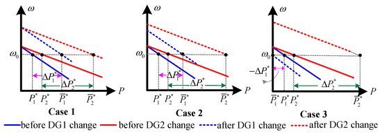
Figure 2. Three cases when $P^{*}$ changes.

• Case 1: $\Delta$P${}_i^{*}$/K${}_i^{}$ = $\Delta$P${}_j^{*}$/K${}_j^{}$. Because C > 0 is always true, it perfectly inherits the frequency synchronization capability of primary control;
• Case 2: $\Delta$P${}_i^{*}$/K${}_i^{}$≠$\Delta$P${}_j^{*}$/K${}_j^{}$ and the conditions in (9) are satisfied. At this point, the synchronization of system frequency can still be achieved, but the synchronization capability is worse than the primary control. This is because as the deviation of $\mid$P${}_i^{*}$/K${}_i^{}-\Delta$P${}_j^{*}$/K${}_j^{}\mid$ increases, the conditions in (9) gradually approach the boundary.
• Case 3: $\Delta$P${}_i^{*}$/K${}_i^{}$≠$\Delta$P${}_j^{*}$/K${}_j^{}$ and the conditions in (9) do not hold with the further increase in the maximum deviation between P${}_i^{*}$/K${}_i^{}$. The microgrid frequency is not synchronized in this case.

To avoid disrupting the frequency convergence capability of the primary droop control, Case 1 is the best choice. It should also be noted that even if $\Delta$P${}_i^{*}$/K${}_i^{}$ = $\Delta$P${}_j^{*}$/K${}_j^{}$, P${}^{*}$ cannot continuously increase (or decrease). This is because in a physical system, parameters such as P and $\omega$ are bounded.

The variation of the droop coefficient K can be equivalently converted to the change in P${}^{*}$. Assuming that the droop coefficient changes $\Delta$K based on (1) we can obtain

$$P_i=[P_i^{*}-\Delta K_i({\omega }_i-{\omega }_0)]-K_i({\omega }_i-{\omega }_0)$$

(12)

Let $\Delta$P${}_i^{*}$ = $\Delta$K${}_i$($\omega$${}_i^{}$−$\omega$${}_0^{}$). Through the above analysis, the frequency synchronization of the physical layer under primary control can be guaranteed when $\Delta$K${}_i$/K${}_i$ = $\Delta$K${}_j$/K${}_j$.

3. Weight-Adaptive Robust Control

The distributed secondary frequency regulation objectives of the information layer are summarized as follows.

• To recovery the angular frequency $\omega$${}_i$ to the nominal value.

  $$\underset{t\to \infty }{lim}{\omega }_i(t)={\omega }_0,\forall i\in V_p$$

  (13)
• To ensure the synchronization stability of the physical layer. According to the analysis presented in Section 2.4, the ideal situation is to make the controllable parameters satisfy

  $$\underset{t\to \infty }{lim}\frac{\Delta P_i^{*}}{K_i}=\frac{\Delta P_j^{*}}{K_j},\underset{t\to \infty }{lim}\frac{\Delta K_i}{K_i}=\frac{\Delta K_j}{K_j},\forall i,j\in V_p$$

  (14)

3.1. Distributed Implementation of Control Objectives

To synchronize the microgrid frequency to $\omega$${}_0$, a distributed consensus control protocol that considers time delays of the information layer is proposed as follows.

$$\begin{array}{cc}\hfill {\dot{u}}_i& =-\sum _{i,j\in V_{in},j\in N_{ni}}{\tilde{a}}_{ij}({\omega }_i(t-{\tau }_{ij})-{\omega }_j(t-{\tau }_{ji}))\hfill \\ \hfill & +g({\omega }_0-{\omega }_i(t-{\tau }_{ij}))+\frac{1}{K_i}{\dot{P}}_i(t)\hfill \end{array}$$

(15)

where g is a positive constant. V${}_{in}$ is the set of agents in the information layer, which is equal to V${}_p$ because of the one-to-one correspondence between DGs and agents. N${}_{ni}$ is the set of neighbor agents of agent i. ${\tau }_{ij}$ represents the constant communication delay between agent i and agent j and ${\tau }_{ij}$ = ${\tau }_{ji}$ = $\tau$. $\tilde{a}$${}_{ij}$ represents the weighted coefficient between agent i and agent j.

To ensure the frequency synchronization stability of the physical layer, $\Delta K$ is set as 0 in this paper, and the control of $\Delta P^{*}$ is implemented by a consensus protocol as

$$\frac{\Delta {\dot{P}}_i^{*}(t)}{K_i}=-\sum _{i,j\in V_{in},j\in N_{ni}}{\tilde{a}}_{ij}(\frac{\Delta P_i^{*}(t-{\tau }_{ij})}{K_i}-\frac{\Delta P_j^{*}(t-{\tau }_{ji})}{K_j})$$

(16)

where $\Delta {\dot{P}}^{*}=\dot{P}$ under the fast dynamic response of the converters.

Then, the distributed frequency controller of the islanded microgrid can be described as

$$P_i(t)=P_i^{*}-K_i({\omega }_i(t)-{\omega }_0)+K_i{u}_i$$

(17)

where the primary control is considered to operate in real time due to the extremely short sampling delay. The information layer control command K${}_i$u${}_i$ causes a change in the nominal active power. According to the above analysis, we know that

$$\Delta P_i^{*}=K_i{u}_i$$

(18)

In (15) and (16), the weight coefficients directly affect the control performance categories, such as stability, convergence speed, and delay robustness, so their design is particularly important. Next, we will explore the influence of control parameters on control performance.

3.2. Control Performance Analysis

3.2.1. Convergence Speed

Define an n×n Laplacian matrix $\mathit{L}$${}_n$ = [l${}_{ij}$]${}_{n\times n}$, where l${}_{ii}$ = ${\sum }_{i\ne j}$$\tilde{a}$${}_{ij}$ and l${}_{ij}$ = −$\tilde{a}$${}_{ij}$. Let m eigenvalues of $\mathit{L}$${}_n$ satisfy 0 <${\lambda }_2$≤${\lambda }_3$ ≤ … ≤${\lambda }_m$, where ${\lambda }_2$ and ${\lambda }_m$ are the second eigenvalue and the largest eigenvalue of $L_n$, respectively. According to the properties of the Laplacian matrix, the following lemma can be obtained.

Lemma 2.

(1) Based on the generalization of the Courant–Fischer theorem [32], if ${\mathbf{1}}^T$$\mathit{x}$= 0, one has min{$\mathit{x}$${}^T$$\mathit{L}$${}_n$$\mathit{x}$} = ${\lambda }_2$$\mathit{x}$${}^T$$\mathit{x}$. (2) Let $\mathit{G}=g{\mathit{I}}_n$, where ${\mathit{I}}_n$ is an n-dimensional unit matrix, then$\mathit{x}$${}^T$$({\mathit{L}}_n+\mathit{G})$$\mathit{x}$$\ge g{\mathit{x}}^T\mathit{x}$.

Since the correlation of power and frequency exists in (17), decoupling is required before analysis. Deriving the derivative of (17) and combining it with (15) and (16), we obtain

$$\begin{array}{cc}\hfill {\dot{e}}_i(t)& =-\frac{{\dot{P}}_i(t)}{K_i}+{\dot{u}}_i\hfill \\ \hfill & =-\sum _{j\in N_i}{\tilde{a}}_{ij}[e_i(t-{\tau }_i)-e_j(t-{\tau }_{ji}))]-g{e}_i(t-{\tau }_i)\hfill \end{array}$$

(19)

where $e_i={\omega }_i-{\omega }_0$.

Theorem 1.

For the frequency control system shown in (16) and (19), the relationship between the weight coefficients and the convergence speed satisfies $V(t)$≤$V(0)$ exp(−2min{${\lambda }_2$,g}t), where $V(t)$ is a Lyapunov function, which corresponds to the total deviation of the system, and $V(0)$ is the initial value of $V(t)$.

Proof of Theorem 1.

The matrix form of (16) and (19) can be written as

$$\dot{\mathit{p}}=-{\mathit{L}}_n\mathit{p}$$

(20)

$$\dot{\mathit{e}}=-({\mathit{L}}_n+\mathit{G})\mathit{e}$$

(21)

where $\mathit{p}=[\Delta P_1^{*}/K_1-p_0,\dots ,\Delta P_q^{*}/K_q-p_0]$, $\mathit{e}$ = [e${}_1$,…,e${}_q$]${}^T$, and $p_0=1/q\sum \Delta (P_i^{*}/K_i)$. q represent the number of agents in the information layer.

Define a Lyapunov function as

$$V=\frac{1}{2}({\mathit{p}}^T\mathit{p}+{\mathit{e}}^T\mathit{e})$$

(22)

This then yields

$$\dot{V}={\mathit{p}}^T\dot{\mathit{p}}+{\mathit{e}}^T\dot{\mathit{e}}=-{\mathit{p}}^T{\mathit{L}}_n\mathit{p}-{\mathit{e}}^T({\mathit{L}}_n+\mathit{G})\mathit{e}$$

(23)

Applying (2) and (3) of Lemma 2, we have

$$\begin{array}{cc}\hfill \dot{V}& \le -{\mathit{p}}^T{\lambda }_2\mathit{p}-{\mathit{e}}^{T}g\mathit{e}\le -min\{{\lambda }_2,g\}[{\mathit{p}}^T\mathit{p}+{\mathit{e}}^T\mathit{e}]\hfill \\ \hfill & =-2min\{{\lambda }_2,g\}V\hfill \end{array}$$

(24)

By solving the differential equation, one can observe that

$$V(t)\le V(0)e^{-2min\{{\lambda }_2,g\}t},$$

(25)

which completes the proof. □

The results show that the total deviation ($V(t)$) asymptotically converges to 0 with the speed of 2 min{${\lambda }_2$,g}. To highlight the role of the weight coefficients, ${\lambda }_2\le g$ is set in this study.

3.2.2. Delay Robustness

Delay robustness refers to the ability of the control system to maintain stable operation under the influence of a time delay. It can be simply measured by means of indicators such as the volatility and stability of the output results.

Since (16) is a special case of (19) with g = 0, only the delay robustness of (19) needs to be investigated.

Theorem 2.

The consensus protocol depicted in (19) is globally asymptotically stable if τ<$[\pi /(2{\lambda }_m$ + $2g$)] is satisfied.

Proof of theorem 2.

After the Laplace transform, (19) can be written as

$$\begin{array}{cc}\hfill s{e}_i(s)-e_i(0)& =-\sum _{j\in N_i}{\tilde{a}}_{ij}{e}^{-\tau s}(e_i(s)-e_j(s))-g{e}^{-\tau s}{e}_i(s)\hfill \end{array}$$

(26)

Its matrix form is

$$\mathit{e}(s)[(s+g{e}^{-\tau s}){\mathit{I}}_n+e^{-\tau s}{\mathit{L}}_n]=e(0)$$

(27)

Let

$$\mathit{F}(s)=(s+g{e}^{-\tau s}){\mathit{I}}_n+e^{-\tau s}{\mathit{L}}_n$$

(28)

Then, the system is stable if and only if all zeros of $\mathit{F}(s)$ are on the open left-half complex plane. Let ${\mathit{v}}_k$ (${\mathit{v}}_k$≠ 0) represent an eigenvector of ${\mathit{L}}_n$ associated with the eigenvalue ${\lambda }_k$. If s i zero, we obtain

$$\mathit{F}(s){\mathit{v}}_k=[(s+g{e}^{-\tau s})+e^{-\tau s}{\lambda }_k]{\mathit{v}}_k=0$$

(29)

which is equivalent to

$$(s+g{e}^{-\tau s})+e^{-\tau s}{\lambda }_k=0$$

(30)

when the delay time reaches its upper bound, the system is critically stable, and the zeros of $\mathit{F}(s)$ are located on the imaginary axis. Therefore, replacing s in (30) with $jw$ and $-jw$ ($w\ge 0$), respectively, we obtain

$$jw+g{e}^{-jw\tau }+{\lambda }_k{e}^{-jw\tau }=0$$

(31)

$$-jw+g{e}^{jw\tau }+{\lambda }_k{e}^{jw\tau }=0$$

(32)

Multiplying the above two equations and using the Euler transform, we have

$$w^2+{(g+{\lambda }_k)}^2-2w(g+{\lambda }_k)sin(w\tau )=0$$

(33)

which is equivalent to

$${(w-(g+{\lambda }_k))}^2+2w(g+{\lambda }_k)(1-sin(w\tau ))=0$$

(34)

Since w, g, and ${\lambda }_k$ are greater than 0, the latter equation holds when

$$w-(g+{\lambda }_k)=0and1-sin(w\tau )=0$$

(35)

that is

$$w=g+{\lambda }_{k}andw\tau =2k\pi +1/2\pi (k=1,2,\dots )$$

(36)

To ensure the stability of the system, $\tau$ satisfies

$$\tau <min\{\frac{2k\pi +1/2\pi }{g+{\lambda }_k}\}=\frac{\pi }{2g+2{\lambda }_m}$$

(37)

Thus, the proof is completed. □

The delay time of (16), $\tau <\frac{\pi }{2{\lambda }_m}$, can be easily obtained when g = 0. Thus, the sufficient delay time of the entire system satisfies

$$\tau <min\{\frac{\pi }{2{\lambda }_m},\frac{\pi }{2{\lambda }_m+2g}\}=\frac{\pi }{2{\lambda }_m+2g}$$

(38)

This indicates that the upper bound of the delay time is inversely proportional to the sum of the largest eigenvalue ${\lambda }_m$ and g. The larger the value of ${\lambda }_m$, the worse the delay robustness of the system.

3.3. Weight-Adaptive Robust Control

In order to improve the convergence speed, the authors of previous studies have always set larger weight coefficients, which may lead to a decrease in delay robustness. Taking a four-node communication network in Figure 3 as an example, we analyze the widely used improved weight coefficient design method proposed in [17].

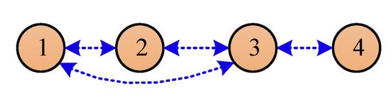
Figure 3. A four-node communication network.

In the classic Metropolis method [33], the weight coefficients are set as

$$a_{ij}=\frac{1}{\max (n_i,n_j)+1},i,j\in V_{in},j\in N_{ni}$$

(39)

where $n_i$ is the number of neighboring agents of agent i. The corresponding Laplacian matrix of Figure 3 is

$$L_{n1}=\left(\begin{array}{cccc}\frac{1}{3}+\frac{1}{4}& -\frac{1}{3}& -\frac{1}{4}& 0\\ -\frac{1}{3}& \frac{1}{3}+\frac{1}{4}& -\frac{1}{4}& 0\\ -\frac{1}{4}& -\frac{1}{4}& \frac{3}{4}& -\frac{1}{4}\\ 0& 0& -\frac{1}{4}& \frac{1}{4}\end{array}\right)$$

(40)

Its second eigenvalue and largest eigenvalue are 0.25 and 1, respectively. If we set g = 0.5, then under the control of (15), the convergence speed of the system in its ideal operating state is 0.5, and the upper bound of the delay time is $\pi /3$(s).

Under the improved method of [17], the weight coefficients are updated as

$$a_{ij}=\frac{2}{n_i+n_j+ϵ},i,j\in V_{in},j\in N_{ni}$$

(41)

where $ϵ$ is a very small number. We set $ϵ$=0.1 and obtain the laplace matrix corresponding to Figure 3 as follows:

$$L_{n2}=\left(\begin{array}{cccc}\frac{2}{4.1}+\frac{2}{5.1}& -\frac{2}{4.1}& -\frac{2}{5.1}& 0\\ -\frac{2}{4.1}& \frac{2}{4.1}+\frac{2}{5.1}& -\frac{2}{5.1}& 0\\ -\frac{2}{5.1}& -\frac{2}{5.1}& \frac{4}{5.1}+\frac{2}{4.1}& -\frac{2}{4.1}\\ 0& 0& -\frac{2}{4.1}& \frac{2}{4.1}\end{array}\right)$$

(42)

Its second eigenvalue and largest eigenvalue are 0.449 and 1.703, respectively. At this time, the convergence speed of the system is 0.898, and the upper bound of the delay time is $\pi /4.406$(s). Compared with the classic Metropolis method, the improved method of [17], although improving the convergence speed, leads to a significant decrease in delay robustness.

Based on the above exemplary analysis, we know that there may be conflict between the convergence speed and delay robustness. Emphasizing only one type of performance can make our control of another type ofperformance worse. To achieve a comprehensive trade-off between the two types of control performance, a simple and effective method can be used for adaptive control, so that the weight coefficients can be adaptively adjusted according to the changes in control scenarios or requirements.

Lemma 3.

If ${\lambda }_A$ is the eigenvalue of matrix$\mathit{A}$, then $k{\lambda }_A$ is the eigenvalue of$k\mathit{A}$(where k is a constant).

In the frequency regulation process, we expect the frequency deviation to be quickly reduced to a safe range and to operate robustly within this range. This requires a fast convergence speed when the frequency deviation is large, and good delay robustness when the frequency is within the safe range. To achieve this expectation, according to the properties of the eigenvalues in Lemma 3, an adaptive coefficient c is added to (15) and (16). By combining (15)–(18), we propose a distributed weight-adaptive control strategy as follows.

$$\left\{\begin{array}{c}{P}_i(t)=P_i^{*}-K_i({\omega }_i(t)-{\omega }_0)+K_i{u}_i\hfill \\ {\dot{u}}_i=-c{\displaystyle \sum _{j\in N_i}}{\tilde{a}}_{ij}({\omega }_i(t-{\tau }_i)-{\omega }_j(t-{\tau }_{ji}))\hfill \\ -c{\displaystyle \sum _{j\in N_i}}{\tilde{a}}_{ij}(\frac{\Delta P_i^{*}(t-{\tau }_i)}{K_i}-\frac{\Delta P_j^{*}(t-{\tau }_{ji})}{K_j})+g({\omega }_0-{\omega }_i(t-{\tau }_i))\hfill \end{array}\right.$$

(43)

where c satisfies

$$c=\left\{\begin{array}{cc}{c}_{min}+\frac{\mid \Delta f\mid }{\Delta f_{max}}(c_{max}-c_{min})\hfill & \mid \Delta f\mid \le \Delta f_{max}\hfill \\ c_{max}\hfill & \mid \Delta f\mid >\Delta f_{max}\hfill \end{array}\right.$$

(44)

where $c_{max}$ and $c_{min}$ are the maximum and minimum allowable values of the adaptive coefficient, respectively. $\Delta f$ and $\Delta f_{\max }$ are the microgrid system frequency deviation and the maximum allowable frequency deviation, respectively.

Figure 4 shows the weight-adaptive frequency controller for an islanded microgrid. In our strategy, the weight coefficients can be adaptively changed according to the frequency deviation. When the frequency deviation approaches or exceeds $\Delta f_{\max }$, the fast frequency regulation capability is ensured by the large adaptive coefficient. When the frequency deviation decreases, the weight coefficients are also adaptively reduced, which significantly improves the delay robustness. Through the design of the adaptive coefficient, the convergence speed and the upper bound of the delay time have been changed to 2$c{\lambda }_2$ and $\pi /(2c{\lambda }_m+2g)$, respectively. Compared with the previous studies, two important types of control performance are considered instead of one, and a comprehensive trade-off between convergence speed and delay robustness is achieved.

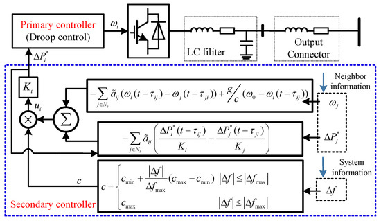
Figure 4. The weight-adaptive frequency controller for an islanded microgrid.

4. Case Studies

To verify the effectiveness of the proposed control strategy, a five-node islanded microgrid is designed here, which consists of four controllable DGs and five loads. The transmission network of the physical layer and the communication network of the information layer are clearly shown in Figure 5. The corresponding system and control parameters are summarized in Table 2.

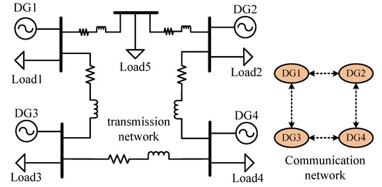
Figure 5. Five-node islanded microgrid test system.

Table 2. Parameters of the test system.

DGs	DG1	DG2	DG3	DG4
$K_i$	0.55 $\times {10}^4$	0.55 $\times {10}^4$	1.1 $\times {10}^4$	1.1 $\times {10}^4$
$P_i^{*}$	2.5 kW	5 kW	5 kW	2.5 kW
Loads	load1	load2/4	load3	load5
	30 kW	5 kW	4 kW	4 kW
Others	$g$	$c_{max}/c_{min}$	$\Delta f_{max}$	Lines
	0.7	1.0/0.7	0.1 Hz	0.15 + j0.3 $\mathsf{\Omega }$

Of course, even if the line impedances in Table 2 were different, this would not affect the stable implementation of the control strategy. This is because $y_{ij}$>0 is always true as long as there is impedance in the transmission lines. According to the system stability conditions in (9), C > 0 is always established, which indicates that the AC voltage and impedance do not affect the effectiveness of the frequency control strategy. In addition, the weight coefficient ${\tilde{a}}_{ij}$ is designed by (39). Through the above analysis, the convergence speed and the upper bound delay time are 1.33c and $\pi /(2.67c+1.4)$(s), respectively.

4.1. Study 1: The Realization of Control Objectives

In order to verify the system’s capability to realize control objectives, a simulation scenario was designed as follows: (1) 0–0.5 s, only the primary control is activated; (2) 0.5–2 s, the proposed adaptive secondary control is activated to participate in frequency support; (3) at 2 s, load 5 is increased by 6 kW; (4) at 3.5 s, load 5 is decreased by 6 kW. In this scenario, we set the delay time $\tau =0.2$ s and obtained the dynamic response results as shown in Figure 6. It can be observed in Figure 6a that the proposed strategy synchronized the frequency to 50 Hz, which could be achieved even if load disturbances occurred. Figure 6c depicts the dynamic changes in $\Delta P_i^{*}$. Using our strategy, $\Delta P_i^{*}/K_i$ can always achieve synchronization after stabilization, which indicates that the frequency synchronization stability of the physical layer is effectively guaranteed. Affected by frequency deviations in Figure 6a, the adaptive coefficient c is dynamically adjusted in Figure 6d. Obviously, even if weight coefficients are constantly changing, control objectives 1 and 2 can be accurately implemented.

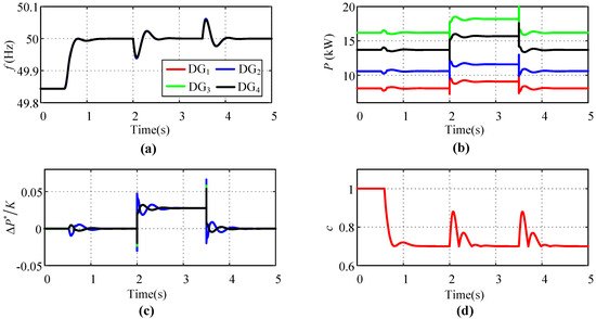
Figure 6. The dynamic responses of study 1 with delay time $\tau$=0.2 s: (a) frequency; (b) active power; (c) ratio of the incremental of power’s nominal valueto the droop coefficient; (d) adaptive coefficient.

4.2. Study 2: Convergence Speed

To verify the convergence performance, we compared the proposed strategy with the classical feedback linearization strategy in [8]. Figure 7 presents a comparison of the frequency and the active power of DG1. It can be observed from the simulation results that the convergence speeds of the two strategies were exactly the same when the frequency deviation was greater than 0.1 Hz. Furthermore, when the deviation was less than 0.1 Hz, the convergence speed of the proposed strategy was theoretically slower than that of the feedback linearization control method. However, due to the 0.2 s delay time, the speed difference between the two strategies was not that large. This is because the classical strategy showed worse robustness in the face of time delays (more shocking results are shown in Study 3). Compared with the classical strategy, the proposed strategy can be stabilized earlier in relation to the nominal value due to the inconspicuous overshoot and oscillation times.

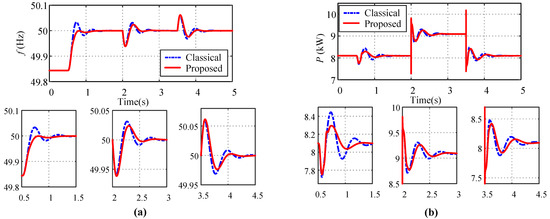
Figure 7. Comparison of convergence speed between the proposed strategy and the classical feedback linearization strategy when $\tau$ = 0.2 s: (a) frequency of DG1; (b) active power of DG1.

4.3. Study 3: Delay Robustness

Compared with the linearization feedback strategy presented in [8], the most obvious advantage of the proposed strategy is its delay robustness. Figure 8 depicts the dynamic responses of frequency and nominal active power with a delay time of 0.5 s. Under the classical strategy, due to the increase in the delay time, the frequency fluctuations shown in Figure 8a were more serious than those shown in Figure 7a, and $\Delta P^{*}/K$ was not synchronized until approximately 2 s had passed.In contrast, the proposed strategy achieved the synchronization of $\Delta P^{*}/K$ in less than 1.5 s, which not only significantly improved the robustness, but also greatly reduced the regulation time.

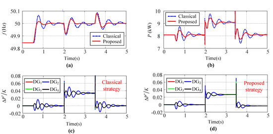
Figure 8. Comparison of the delay robustness of the proposed strategy and that of the classical feedback linearization strategy when $\tau$ = 0.5 s: (a) frequency of DG1; (b) output active power of DG1; (c) $\Delta P_i^{*}/K_i$ of the feedback linearization strategy; (d) $\Delta P_i^{*}/K_i$ of the proposed strategy.

When further increasing the delay time to 1 s, we obtained the simulation results shown in Figure 9. Under the classical strategy, even without the addition of load disturbances, the system cannot run stably, because the upper bound of the delay time is $\pi /(2.67+1.4)$ = 0.77 s < 1. In contrast, when the frequency was synchronized to 50 Hz, the upper bound of the delay time of the proposed strategy was increased to 1.1 s. Therefore, the stability of the frequency can still be guaranteed, and the synchronization of $\Delta P^{*}/K$ can also be realized.

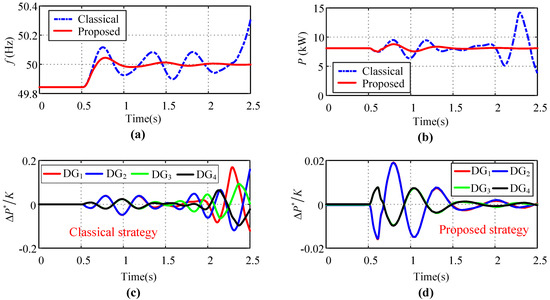
Figure 9. Comparison of delay robustness of the proposed strategy and that of the classical feedback linearization strategy when $\tau$ = 1 s: (a) frequency of DG1; (b) output active power of DG1; (c) $\Delta P_i^{*}/K_i$ of the feedback linearization strategy; (d) $\Delta P_i^{*}/K_i$ of the proposed strategy.

5. Conclusions

A weight-adaptive robust control strategy, which realizes a comprehensive trade-off between convergence speed and delay robustness, is proposed for the distributed frequency regulation of islanded microgrids. Improvementsnot only in frequency restoration, but also in the design of the controllable parameters are proposed here through the analysis of the frequency synchronization stability in the physical layer. We have also investigated the relationship between weight coefficients and two important control properties, and established the convergence speed and the upper bound of the delay time. An adaptive coefficient, which can vary with frequency deviations, was added to the proposed strategy to achieve a trade-off between convergence speed and delay robustness. The simulation results showed that, compared with the classical feedback linearization strategy, the delay robustness of the proposed strategy was significantly improved under the guarantee of a good convergence speed. In our future work, we will consider more control performance categories, such as the robustness of noise influences or uncertain topologies. In addition, research on how to apply the proposed strategy to energy management systems [34,35,36] in real-world microgrids is also an important direction of study in the future.

References

- Aznavi, S.; Fajri, P.; Sabzehgar, R.; Asrari, A. Optimal management of residential energy storage systems in presence of intermittencies. J. Build. Eng. 2020, 29, 101149. [Google Scholar] [CrossRef]
- Kumtepeli, V.; Zhao, Y.; Naumann, M.; Tripathi, A.; Wang, Y.; Jossen, A.; Hesse, H. Design and analysis of an aging-aware energy management system for islanded grids using mixed-integer quadratic programming. Int. J. Energy Res. 2019, 43, 4127–4147. [Google Scholar] [CrossRef]
- Iris, C.; Lam, J.S.L. Optimal energy management and operations planning in seaports with smart grid while harnessing renewable energy under uncertainty. Omega 2021, 103, 102445. [Google Scholar] [CrossRef]
- Hussain, A.; Choi, I.S.; Im, Y.H.; Kim, H.M. Optimal Operation of Greenhouses in Microgrids Perspective. IEEE Trans. Smart Grid 2019, 10, 3474–3485. [Google Scholar] [CrossRef]
- Du, Y.; Tu, H.; Lukic, S. Distributed Control Strategy to AchieveSynchronized Operation of an Islanded MG. IEEE Trans. Smart Grid 2019, 10, 4487–4496. [Google Scholar] [CrossRef]
- Lassater, R.H. Smart distribution: Coupled microgrids. Proc. IEEE. 2011, 99, 1074–1082. [Google Scholar] [CrossRef]
- Zhang, H.; Meng, W.; Qi, J.; Wang, X.; Zheng, W. Distributed Load Sharing Under False Data Injection Attack in an Inverter-Based Microgrid. IEEE Trans. Ind. Electron. 2019, 66, 1543–1551. [Google Scholar] [CrossRef]
- Karimi, M.; Wall, P.; Mokhlis, H.; Terzija, V. A New Centralized Adaptive Under-frequency Load Shedding Controller for Microgrids Based on a Distribution State Estimator. IEEE Trans. Power Del. 2017, 32, 370–380. [Google Scholar] [CrossRef]
- Babqi, A.J.; Yi, Z.; Etemadi, A.H. Centralized finite control set model predictive control for multiple distributed generator small-scale microgrids. In Proceedings of the 2017 North American Power Symposium (NAPS), Morgantown, WV, USA, 17–19 September 2017. [Google Scholar]
- Serban, I.; Marinescu, C. Aggregate load-frequency control of a wind-hydro autonomous microgrid. Renew. Energy 2011, 36, 3345–3354. [Google Scholar] [CrossRef]
- Bidram, A.; Davoudi, A.; Lewis, F.L.; Guerrero, J.M. Distributed Cooperative Secondary Control of Microgrids Using Feedback Linearization. IEEE Trans. Power Syst. 2013, 28, 3462–3470. [Google Scholar] [CrossRef] [Green Version]
- Bidram, A.; Davoudi, A.; Lewis, F.L. A Multiobjective Distributed Control Framework for Islanded AC Microgrids. IEEE Trans. Ind. Informat. 2014, 10, 1785–1798. [Google Scholar] [CrossRef]
- Simpson-Porco, J.W. Secondary Frequency and Voltage Control of Islanded Microgrids via Distributed Averaging. IEEE Trans. Ind. Electron. 2015, 62, 7025–7038. [Google Scholar] [CrossRef]
- Zhang, Z.; Chow, M.Y. Convergence Analysis of the Incremental Cost Consensus Algorithm Under Different Communication Network Topologies in a Smart Grid. IEEE Trans. Power Syst. 2012, 27, 1761–1768. [Google Scholar] [CrossRef]
- Morstyn, T.; Savkin, A.V.; Hredzak, B.; Agelidis, V.G. Multi-Agent Sliding Mode Control for State of Charge Balancing Between Battery Energy Storage Systems Distributed in a DC Microgrid. IEEE Trans. Smart Grid 2018, 9, 4735–4743. [Google Scholar] [CrossRef] [Green Version]
- Azevedo, R.D.; Cintuglu, M.H.; Ma, T.; Mohammed, O.A. Multiagent-Based Optimal Microgrid Control Using Fully Distributed Diffusion Strategy. IEEE Trans. Smart Grid 2017, 8, 1997–2008. [Google Scholar] [CrossRef]
- Xu, Y.; Liu, W. Novel Multiagent Based Load Restoration Algorithm for Microgrids. IEEE Trans. Smart Grid 2011, 2, 152–161. [Google Scholar] [CrossRef]
- Xu, Y.; Li, Z. Distributed Optimal Resource Management Based on the Consensus Algorithm in a Microgrid. IEEE Trans. Ind. Electron. 2015, 62, 2584–2592. [Google Scholar] [CrossRef]
- Zuo, S.; Davoudi, A.; Song, Y.; Lewis, F.L. Distributed Finite-Time Voltage and Frequency Restoration in Islanded AC Microgrids. IEEE Trans. Ind. Electron. 2016, 63, 5988–5997. [Google Scholar] [CrossRef]
- Dehkordi, N.M.; Sadati, N.; Hamzeh, M. Distributed Robust Finite-Time Secondary Voltage and Frequency Control of Islanded Microgrids. IEEE Trans. Power Syst. 2017, 32, 3648–3659. [Google Scholar] [CrossRef]
- Chen, G.; Zhao, Z. Delay Effects on Consensus-Based Distributed Economic Dispatch Algorithm in Microgrid. IEEE Trans. Power Syst. 2018, 33, 602–612. [Google Scholar] [CrossRef]
- Chen, G.; Guo, Z. Distributed Secondary and Optimal Active Power Sharing Control for Islanded Microgrids with Communication Delays. IEEE Trans. Smart Grid 2019, 10, 2002–2014. [Google Scholar] [CrossRef]
- Liu, W.; Gu, W.; Sheng, W.; Meng, X.; Xue, S.; Chen, M. Pinning-Based Distributed Cooperative Control for Autonomous Microgrids Under Uncertain Communication Topologies. IEEE Trans. Power Syst. 2016, 31, 1320–1329. [Google Scholar] [CrossRef]
- Tang, Z.; Hill, D.J.; Liu, T. A Novel Consensus-Based Economic Dispatch for Microgrids. IEEE Trans. Ind. Appli. 2018, 9, 3920–3922. [Google Scholar] [CrossRef]
- Zhang, X.; Xu, H.; Yu, T.; Yang, B.; Xu, M. Robust collaborative consensus algorithm for decentralized economic dispatch with a practical communication network. Electr. Power Syst. Res. 2016, 140, 597–610. [Google Scholar] [CrossRef]
- Dong, J.; Xue, X. Synchronization analysis of Kuramoto oscillators. Commun. Math. Sci. 2013, 11, 465–480. [Google Scholar] [CrossRef] [Green Version]
- Simpson-Porco, J.W.; Dörfler, F.; Bullo, F. Synchronization and power sharing for droop-controlled inverters in islanded microgrids. Automatica 2013, 49, 2603–2611. [Google Scholar] [CrossRef] [Green Version]
- Dörfler, F.; Bullo, F. Kron Reduction of Graphs With Applications to Electrical Networks. IEEE Trans. Circuits Syst. Regul. Pap. 2013, 60, 150–163. [Google Scholar] [CrossRef] [Green Version]
- Song, H.H.; Han, L.K.; Wang, Y.C.; Wen, W.F.; Qu, Y.B. Kron Reduction Based on Node Ordering Optimization for Distribution Network Dispatching with Flexible Loads. Energies 2022, 15, 2964. [Google Scholar] [CrossRef]
- Cady, S.T.; Dominguez-Garcia, A.D.; Hadjicostis, C.N. A Distributed Generation Control Architecture for Islanded AC Microgrids. IEEE Trans. Control Syst. Technol. 2015, 23, 1717–1735. [Google Scholar] [CrossRef]
- Liu, Y.; Qu, Z.; Xin, H.; Gan, D. Distributed Real-Time Optimal Power Flow Control in Smart Grid. IEEE Trans. Power Syst. 2017, 32, 3403–3414. [Google Scholar] [CrossRef]
- Olfati-Saber, R.; Fax, J.A.; Murray, R.M. Consensus and cooperation in networked multi-agent systems. Proc. IEEE 2007, 95, 215–233. [Google Scholar] [CrossRef] [Green Version]
- Xiao, L.; Boyd, S.; Kim, S.J. Distributed average consensus with least-mean-square deviation. Presented at the 17th International Symposium on Mathematical Theory of Networks and Systems, Kyoto, Japan, 24–28 July 2006. [Google Scholar]
- Jose, M.R.A.; Najmeh, B.; Juan, G.A.C.; Doris, S.; Juan, C.V.; Josep, M.G. Energy management system optimization in islanded microgrids: An overview and future trends. Renew. Sustain. Energy Rev. 2021, 149, 111327. [Google Scholar]
- Iris, C.; Jasmine, S. A review of energy efficiency in ports: Operational strategies, technologies and energy management systems. Renew. Sustain. Energy Rev. 2019, 112, 170–182. [Google Scholar] [CrossRef]
- Kafetzis, A.; Ziogou, C.; Panopoulos, K.D.; Papadopoulou, S.; Seferlis, P.; Voutetakis, S. Energy management strategies based on hybrid automata for islanded microgrids with renewable sources, batteries and hydrogen. Renew. Sustain. Energy Rev. 2020, 134, 110118. [Google Scholar] [CrossRef]
Publisher’s Note: MDPI stays neutral with regard to jurisdictional claims in published maps and institutional affiliations. |
© 2022 by the authors. Licensee MDPI, Basel, Switzerland. This article is an open access article distributed under the terms and conditions of the Creative Commons Attribution (CC BY) license (https://creativecommons.org/licenses/by/4.0/).