Abstract
The role of hydropower has become increasingly essential following the introduction of intermittent renewable energies. Quickly regulating power is needed, and the transient operations of hydropower plants have consequently become more frequent. Large pressure fluctuations occur during transient operations, leading to the premature fatigue and wear of hydraulic turbines. Investigations of the transient flow phenomena developed in small-scale turbine models are useful and accessible but limited. On the other hand, experimental and numerical studies of full-scale large turbines are challenging due to production losses, large scales, high Reynolds numbers, and computational demands. In the present work, the operation of a 10 MW Kaplan prototype turbine was modelled for two operating points on a propeller curve corresponding to the best efficiency point and part-load conditions. First, an analysis of the possible means of reducing the model complexity is presented. The influence of the boundary conditions, runner blade clearance, blade geometry and mesh size on the numerical results is discussed. Secondly, the results of the numerical simulations are presented and compared to experimental measurements performed on the prototype in order to validate the numerical model. The mean torque and pressure values were reasonably predicted at both operating points with the simplified model. An analysis of the pressure fluctuations at part load demonstrated that the numerical simulation captured the rotating vortex rope developed in the draft tube. The frequencies of the rotating and plunging components of the rotating vortex were accurately captured, but the amplitudes were underestimated compared to the experimental data.
1. Introduction
The introduction of intermittent renewable energy resources such as wind and solar power requires additional power to regulate grid frequency. Hydropower is often used to regulate grid frequency because hydraulic turbines can operate in a relatively wide range of power outputs and load changes and they are able to start and stop in a matter of seconds and minutes, respectively. Such use of hydropower is relatively new and imposes constraints on the hydraulic turbines for which they were not initially designed [1,2]. This may lead to some premature wear and sometimes failures because of large pressure fluctuations mainly arising in the draft tube. A lot of research is now dedicated to minimizing the effect of operating regimes away from the best efficiency and transient operation. The flow phenomena leading to large pressure pulsations need to be well-understood to allow for the development of technology capable of mitigating them. The investigations of such new operating conditions and mitigation techniques are challenging, as the consequences may be both hydrodynamic and structural.
Most studies related to the effect of off-design operations and transients have been performed with model testing and numerical simulations of these model turbines. Model testing allows for the investigation of turbines in a wide range of precise and repeatable operating conditions. Detailed pressure, strain and velocity measurements can now be performed on such turbine models. Extensive measurement campaigns have been carried out, predominantly focusing on Francis turbine models [3,4,5,6] but also a bulb model [7,8] and a Kaplan turbine model [9,10].
Ideally, the investigation of hydraulic turbines should be performed on the prototype itself. However, such experiments are challenging because of both the large scales involved and the costs, mainly because of the production losses. There are only a handful of studies concerning full-scale turbines available in the literature [11,12]. None of them offer the same level of detail as experiments performed on models where optical methods may be used for velocity measurements. Usually, full-scale measurements are limited to pressure and strain measurements in the stationary domain [13,14]. Performing measurements on a runner [15,16], presents another level of difficulty available in few studies. Numerical simulations can provide additional information otherwise difficult to obtain from measurements. Together, both types of investigation can contribute to developing data-driven control solutions that optimize the operation and diagnosis of hydraulic machine failures [17,18]. However numerical studies concerning full-scale hydraulic turbines are also sparse. Such simulations are challenging because of the large dimensions, high Reynolds numbers, and lack of experimental data to validate the results [19,20]. There have been no numerical studies referring to full-scale Kaplan prototype turbines.
The advancement in computer hardware, hydraulic numerical simulations and turbulence modelling may currently allow for the easier handling of prototype simulations. Nonetheless, there is a growing need to simplify the numerical models to obtain results in a reasonable amount of time with a reasonable accuracy.
The present work introduces the numerical simulation of a full-scale 10 MW Kaplan turbine prototype at two operating points on a propeller curve. The chosen operating conditions are equivalent to the best efficiency point and part-load operating condition of a single regulated turbine, such as Francis and propeller types. The potential to decrease model complexity was addressed by investigating several issues such as boundary conditions, runner blade clearance, blade geometry and mesh size. The different parameters were systematically investigated to assess their impact on the numerical accuracy of the simulation. The aim was to optimize the numerical accuracy, computational demands, and simulation time. The reduced model was validated using experimental data measured with the corresponding Kaplan prototype.
2. Experimental Measurements
2.1. The Porjus U9 Prototype
An experimental investigation was performed on the Porjus U9 Kaplan turbine prototype by Soltani et al. [1]. This unit is part of the Porjus Hydropower Center, situated in the north of Sweden, and it is primarily used for educational and research purposes. The Porjus U9 Kaplan turbine presented in Figure 1 has 6 runner blades, 20 equally spaced guide vanes, and 18 unequally distributed stay vanes. The runner has a diameter of 1.55 m and is located approximately 7 m below the tailwater. Table 1 presents the rated parameters of the turbine.
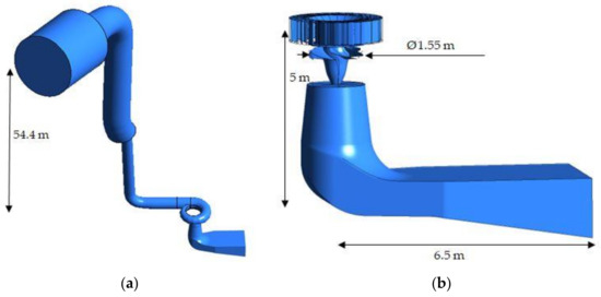
Figure 1.
The main dimensions of the Porjus U9 Kaplan turbine prototype: (a) complete turbine geometry; (b) stay vanes, guide vanes, runner and draft tube.

Table 1.
Rated parameters of the Porjus U9 prototype Kaplan turbine.
2.2. Experimental Setup
The operating points investigated in this paper were part of a measurement campaign performed on the Porjus U9 Kaplan turbine to study different load variations and steady-state operations. Twelve miniature piezoresistive pressure transducers (Kulite LL-080 series) were mounted on small capsules (3 mm in diameter and 5 mm in height) glued on the pressure side (from PS1 to PS6) and on the suction side (from SS1 to SS6) of one runner blade (Figure 2a). An epoxy layer was then added to the blade pressure and suction sides to create a smooth surface (Figure 2b). A similar epoxy layer was applied to the opposite blade to avoid the hydraulic and mass unbalance resulting from the weight of the applied epoxy on the instrumented blade. The pressure transducers were located at the intersection of imaginary circles that passed through 1/3 and 2/3 of the blade’s span and 1/4, 1/2, and 3/4 of the blade’s chord lines. The operating range of the pressure transducers was 0–700 kPa, and their natural frequency was 380 kHz. Two torsion strain gages (K-XY41-6/350-3-2M manufactured by HBM) were installed on the turbine shaft between the turbine guide bearing and the generator guide bearing to measure the shaft torsional strain. The resistance and gage factor of the torsional strain gages were 350 ± 0.35% and 2.08 ± 1%, respectively. A detailed description of the data-acquisition system, additional sensors, and operating conditions used in this measurement campaign was provided by Soltani et al. [1].
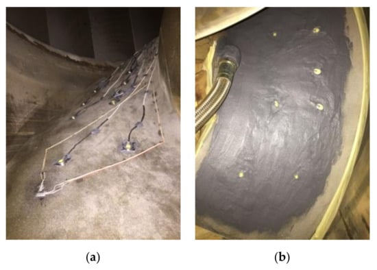
Figure 2.
(a) Pressure transducers mounted on the runner blade; (b) epoxy layer added to the runner blade. The hydraulic hose was used to protect the cables from the blade to the runner cone.
The uncertainty analysis for the pressure transducers and strain gages was conducted using six nonconsecutive repeated measurements at the best efficiency point. The uncertainties of the pressure transducers and torsion strain gage installed on the shaft are presented in Soltani et al. [1].
2.3. Measuring Program
In this study, two experimentally investigated operating points, located on a propeller curve for a fixed blade angle β = −4.2°, were selected. The first operating point (OP1) is located on the left side of the propeller curve. It was characterized by a low discharge and the presence of a rotating vortex rope (RVR). The second operating point (OP2) was closer to the best efficiency point and presented a larger discharge. OP1 and OP2 are considered to be the part-load operating point and best efficiency point, respectively. The operating parameters are listed in Table 2.
Table 2.
Operating condition parameters.
The experimental power values recorded during the measurement campaign presented in [1] were adjusted according to the values recorded in the power plant control room. Furthermore, the control room recordings were validated by index measurements.
3. Numerical Simulations Setup
Several numerical models were evaluated before performing the final simulations at OP1 and OP2. The object was to minimize the computational cost associated with the prototype dimensions and high Reynolds number and to address the uncertainty associated with the experimental data used as boundary conditions. This chapter follows the investigations performed in this study to reduce the model complexity instead of the classical sequence of geometry, mesh, boundary conditions and flow modelling. Therefore, the flow modelling is firstly presented, followed by a description of the main boundary conditions, different geometries used, and the mesh sensitivity analysis.
The different issues considered in these numerical models were the boundary conditions, mesh sensitivity, and numerical error and the influence of the runner blade clearance, epoxy layer added to two blades, and runner blade angle.
The influence of the boundary conditions was proven significant in previous studies [21,22,23] showing that specifying a constant total pressure at the inlet of the numerical domain improved the accuracy of the numerical results. To have a better estimation of the total pressure at the inlet of the investigated domain, a steady simulation was first carried out to evaluate the pressure losses in the upstream geometry comprising the spiral casing and penstock.
A mesh sensitivity analysis was performed to find a good compromise between the spatial discretization, the numerical error, and the computational resources. The same arguments led to the investigation of the runner blade clearance modelling, as the discretization of a very small volume considerably increases the mesh size and, consequently, the simulation time.
Another investigation focused on the importance of modelling the epoxy layer added to two runner blades during the experimental investigation. Re-building the geometry of the runner blade with an approximation of the epoxy layer is usually time-consuming, and the potential impact on the numerical results had to be assessed.
Finally, as the experimental uncertainty of the measured runner blade angle could not be quantified because the runner could not be scanned during the measurements, a sensitivity analysis was performed on this parameter as well.
Table 3 summarizes the different performed investigations. The following section presents and discusses the equations, boundary conditions, geometry and mesh used in the different setups.
Table 3.
Numerical studies setup summary. The Rayleigh–Plesset cavitation model was employed in all unsteady simulations.
3.1. Flow Modelling
The numerical simulations presented in this paper were carried out using Ansys CFX Solver v16.2. The unsteady Reynolds-averaged Navier–Stokes equations were solved with an element-based finite volume method; therefore, the spatial domain was discretized to build finite volumes. The computational domain was modelled using a hexahedral mesh built in ICEM v16.2 for the guide vane and draft tube domains. The runner was discretized using TurboGrid v16.2, software optimized for the discretization of turbine blade passages. The software allows for the generation of good-quality hexahedral mesh for complex blade geometry.
Combining the advantages of the k-epsilon model in the free stream and k-omega model for the near-wall flow, the k-omega Shear Stress Transport (SST) turbulence model provides a good prediction of flow separation and has been proven to perform well under cavitating conditions [24,25,26]. The k-omega SST model was employed in all numerical simulations presented in this paper. The k-omega SST models the transport of the turbulent shear stress by solving two transport equations (Equations (1) and (2)): one for the turbulent kinetic energy (k) and one for the turbulent frequency (ω). The turbulent viscosity () is modelled according to Equation (3).
where Pk is the production rate of turbulence; Pkb and Pωb represent the influence of the buoyancy forces; β, β’, α, σk, σω1 and σω2 are coefficients of the turbulence model; and F1 and F2 are blending functions that switch from the k-epsilon model to k-omega [27].
The large domain size and high Reynolds number made the resolution of y+ near the value of 1, impossible. However, the average y+ values were kept under 25 because the automatic wall function used for the simulations provides reasonable results when compared to the experimental data [28]. In the unsteady simulations, the advection term was first discretized using the upwind advection scheme to achieve convergence faster. These results were provided as initial conditions to an unsteady simulation employing the high-resolution advection scheme. The high-resolution advection scheme automatically maintained the order of the discretization scheme as close to second order as possible to keep the solution robust and bounded. The second-order backward Euler transient scheme was used in all unsteady simulations. The transient time step was set to correspond to one degree of the runner rotation. The influence of the time step size was previously investigated [23], and other studies showed that time steps corresponding to a runner rotation of 0.5–5° is recommended [2]. Finally, the Rayleigh–Plesset cavitation model [24,29] was employed in consideration of the saturation pressure for a temperature of 12.5 °C, as recorded during the measurement campaign. The numerical modelling of the cavitation was introduced after obtaining large negative pressure values near the leading edge of the runner blade and was expected to improve the modelling of the flow [24].
All above-mentioned numerical simulations were validated against experimental data measured at the best efficiency point, OP2 (see Table 2).
3.2. Boundary Conditions
The constant total pressure was used as the inlet boundary condition of the computational domain based on previous studies [22,23]. The outlet was modelled as an opening with specified pressure and direction. The opening boundary condition allows for flow recirculation when the pressure is imposed. When the flow is leaving the domain, the pressure is considered as the relative static pressure as opposed to the total pressure that is considered when the flow enters the domain. Such boundary conditions allow for a shorter computational domain when the flow direction is not known.
To decrease the computational time, the domain of the turbine included a single stay vane-guide vane passage, the runner, and the draft tube. For a better approximation of the total pressure defined at the inlet of the stay vanes, a steady-state simulation of the flow inside the penstock and spiral casing was performed. A mass flow rate of 13 m3/s was specified at the inlet of the penstock (P), and an opening with 0 Pa relative pressure was defined at the outlet of the spiral casing (SC). A pressure drop of 7874 Pa was obtained between the inlet and the outlet of the domain ), corresponding to an approximate head difference of 0.8 m.
Henceforward, the gross head of the turbine, Hgross, was adjusted in the simulations to consider the static pressure difference between the inlet and the outlet of the computational domain and the pressure losses in the penstock and spiral casing. The total head was calculated as:
where z is the elevation.
The boundary conditions for the turbine simulation were defined according to the experimental measurements performed in [1]. The total pressure of 6.9 bar was fixed at the inlet of the computational domain, and the outlet pressure was set as 2.2 bar.
3.3. Geometry
The Porjus U9 Kaplan turbine (Figure 1) includes a penstock, spiral casing, 18 stay vanes, 20 guide vanes, a runner composed of 6 runner blades, and a draft tube. The geometry was obtained from the scaled model geometry. Several aspects had to be clarified before building the definitive numerical model, each concerning a different geometry setup.
To define the total pressure at the inlet of the stay vanes, a steady-state simulation of the flow inside the penstock and spiral casing was first carried out, and the pressure losses throughout this domain were obtained. The computational domain for this investigation is presented in Figure 1a. The large inlet pipe corresponds to the penstock of an older turbine that had a larger flow rate. The smaller pipe was installed with the Porjus U9 turbine.
The modelling of the runner blade clearance required a larger mesh size and, therefore, higher computational demands because of the very small scales involved. The influence of the runner blade clearance size on the numerical results was investigated. Table 4 presents the relative dimensions of the three clearance sizes considered: no clearance, constant clearance near the hub and shroud, and variable clearance from the leading edge (LE) towards the trailing edge (TE).
Table 4.
Simulated clearance sizes representing percentages of the runner diameter.
A steady numerical simulation was performed to verify whether the layers of epoxy added for the blade instrumentation had a significant impact on the numerical results. The blade geometry was modified to approximate the real blade covered by the epoxy layer (Figure 3). Considering the thickness of the epoxy layer, the blade thickness in the numerical model was accordingly increased by 5 mm with a decreasing thickness toward the edges of the blade. The estimated average width of the inter-blade channel was 200 mm at β = −4.2°. Therefore, the added epoxy narrowed the flow channel by a maximum of 2.5% on each side of the blades.
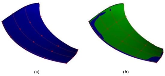
Figure 3.
(a) Runner blade original geometry; (b) geometrical representation of the epoxy layer added for blade instrumentation during the measurements.
As the blade angle (Figure 4) used during the measurements contained a certain amount of uncertainty, a sensitivity analysis was performed to assess its influence on the numerical results. The obtained results were compared to the measurements.
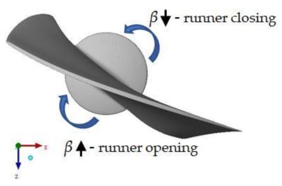
Figure 4.
Runner blade angle variation.
The results of the steady simulations carried out for the different blade angle values provided the initial conditions for the unsteady simulations performed for the two extreme runner blade angles, i.e., the unaltered experimental blade angle (β = −4.2°) and +6°; see Table 5. In order to accelerate the convergence of the numerical solutions, the upwind scheme was first used for the discretization of the advection term before running the unsteady simulations with the high-resolution advection scheme (CFX Pre Modelling Guide).
Table 5.
Simulated runner blade angles. Experimental value β = −4.2°.
Two configurations of the computational domain were used in the numerical studies, one using a single runner blade passage and the second using the entire turbine runner with all six blade passages. The three domains (Figure 5)—one stay vane and guide vane passage, one or six runner blade passages, and the complete draft tube—were connected using stage interfaces, except for the case including the full runner domain where a transient rotor–stator interface was used.
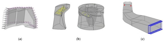
Figure 5.
(a) Stay vane and guide vane domain; (b) runner domain, single blade passage (left), complete runner (right); (c) draft tube domain.
Furthermore, the entire runner domain was modelled, thus allowing for the use of a transient rotor–stator interface between the runner and draft tube domains. This type of interface takes the transient behavior of the flow between domains into account.
Twelve pressure monitor points, corresponding to the locations of the pressure sensors mounted on the blade during the experimental measurements [1], were defined on the runner blade: from PS1 to PS6 on the pressure side and from PS1 to PS6 on the suction side (Figure 5b). Additionally, two diametrically opposed monitor points were defined in the draft tube, DTin and DTout (Figure 5c), to capture the pressure fluctuations due to the formation of the RVR at the part-load operating point (OP1 in Table 2) in the numerical studies.
3.4. Mesh Sensitivity Analysis
Figure 6, Figure 7 and Figure 8 present the meshes created for each computational domain. The hexahedral meshes were built in ICEM v16.2 for all the domains, except for the runner blade passage domain generated with TurboGrid v16.2. The stay vane and guide vane meshes are presented in Figure 6, along with a detail of the boundary layer mesh around the trailing edge of the stay vane and the leading edge of the guide vane.
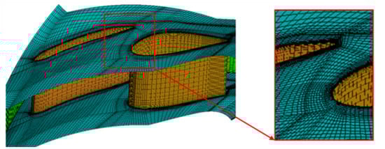
Figure 6.
Stay vane and guide vane mesh (left) and zoom at the trailing edge of the stay vane and the leading edge of the guide vane (right).
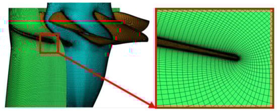
Figure 7.
Runner mesh (left) and zoom at the trailing edge of the stay vane and the leading edge of the guide vane (right).
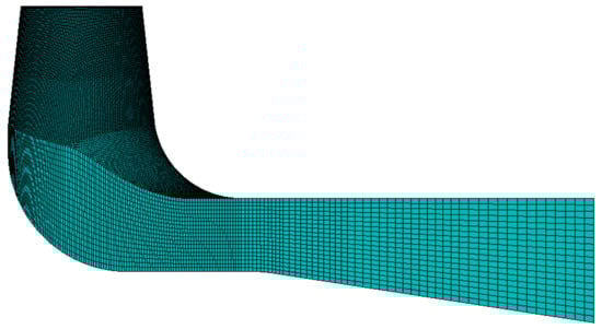
Figure 8.
Draft tube mesh.
Similarly, the discretization of the runner domain and the boundary layer mesh are presented in Figure 7. The runner (Figure 7) and draft tube mesh (Figure 8) underwent mesh sensitivity analyses. The meshes were dimensioned according to the conclusions presented further in this section.
A synthesis of the mesh quality parameters evaluated in Ansys CFX Solver for each computational domain mentioned in the previous section is presented in Table 6. The mesh orthogonality angle represents the minimum angle between two adjacent element faces. The mesh expansion factor is the ratio of the smallest element volume to the largest element volume sharing a node. The mesh aspect ratio is the maximum ratio of the largest to the smallest face area of all the elements sharing a node.
Table 6.
Mesh size and quality parameters of the different meshes used in the simulations.
Steady-state simulations were performed to estimate the numerical error and evaluate the sensitivity of the numerical model to the discretization of the runner and draft tube domains. The investigated model consisted of a single guide vane passage including a stay vane, one runner blade passage and the draft tube. The guide vane was considered to have an insignificant influence on the investigated flow; therefore, a mesh sensitivity analysis was not performed on this domain, as previously employed in a study of the U9 Kaplan model [23].
In the current study, the runner blade angle was modified to fit the prototype experimental value, and the discretization was entirely redone. No clearances were modelled for the mesh sensitivity analysis. Four levels of mesh refinement were investigated, and these are henceforth referred to as R1–R4. The main size and quality parameters of the runner mesh are presented in Table 7. The global size factor defines the overall mesh size and controls the resolution of the mesh in the entire domain, and the edge refinement factor adjusts the resolution of the mesh in the boundary layer.
Table 7.
Runner mesh size and quality parameters.
The torque value obtained with an ‘infinite size’ mesh (T∞) was determined using the Richardson extrapolation. Figure 9 presents the numerical values obtained from the simulations with different levels of mesh refinement of the runner domain. The torque was normalized with the ‘infinite size’ mesh value. The deviation in numerical pressure values was expected to be less than 4% from coarse to fine discretization [14]. Considering that there was no significant difference between the torque results obtained with the two most refined levels of discretization, all the simulations presented following this section employed runner mesh R3, with 1.12 × 10⁶ elements per blade passage.
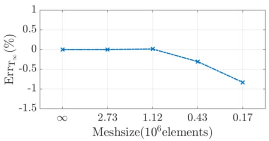
Figure 9.
Variation of the normalized torque with the runner mesh size.
The discretization level of the draft tube domain could influence the numerical results obtained in the runner domain, therefore justifying a mesh sensitivity study and the need to estimate the numerical error induced by the draft tube mesh. Three levels of mesh refinement were investigated, and there are henceforth referred to as DT1–DT3. The draft tube’s primary size and quality parameters are presented in Table 8.
Table 8.
Draft tube mesh size and quality parameters.
Similar to the runner mesh sensitivity study, the torque value obtained with an infinite mesh (T∞) was determined using the Richardson extrapolation. Figure 10 presents the numerical values obtained from the simulations with different levels of mesh refinement of the draft tube domain. The torque was normalized with the infinite mesh value. All the simulations presented after this section employed the draft tube mesh DT3, with 3.18 × 10⁶ elements per blade passage. A 5% discretization error was assumed to be reasonable considering the size of the draft tube mesh.
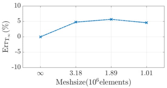
Figure 10.
Variation of the normalized torque with the draft tube mesh size.
4. Results and Discussion
4.1. Runner Clearances
Using the selected runner mesh, R3, steady-state simulations were first performed to investigate the influence of the runner blade clearance.
The values were made dimensionless with the result of the ‘no clearance’ simulation. Figure 11 presents the variation of the torque obtained from the numerical simulations with different types of clearances (Table 4). The ‘constant clearance’ simulation underestimated the torque compared to the other two cases because the ‘constant clearance’ values were the largest, thus allowing for a larger flow rate. The ‘variable clearance’ simulation provided very similar results to the ‘no clearance’ simulation because the real and/or approximated dimensions of the variable clearances were very small and did not impact the torque results. Modelling the variable clearance did not have enough of a significant impact on the numerical results to justify the added computation time.
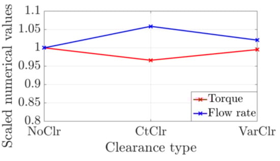
Figure 11.
Variation of the scaled torque and flow rate with the runner blade clearance size.
A parameter found to be significantly influenced by modelling the runner blade clearances was the pressure monitored on the suction side of the blade (SS3), located closer to the shroud and near the trailing edge. The numerical and experimental pressure values were scaled with the reference pressure measured by Soltani et al. [1] with an empty turbine chamber. The results were consistent to the values presented in Table 4. The shroud clearance at the trailing edge was very small and could not be modelled, so the smallest modelled clearance was 0.05% D. This clearance size was used in both the ‘constant clearance’ and the’ variable clearance’ simulation, thus explaining the similar pressure values obtained from the two simulations at SS3 (Figure 12).
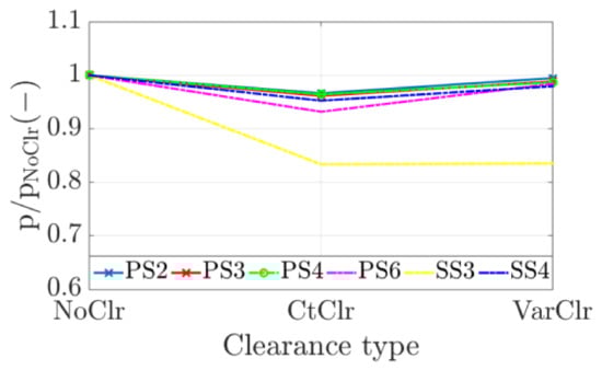
Figure 12.
Variation of the scaled pressure with the runner blade clearance size.
Considering the mesh size, the computational resources required to model the small variable clearances, and the influence of the runner blade clearance on the numerical results, the runner blade clearance was not modelled in further simulations.
4.2. Epoxy Study
An epoxy layer was added to one runner blade to hold the pressure sensors and to a second (opposite) runner blade to balance the runner. The influence of the thickness of the epoxy layer was analyzed. The adjustment of the geometry did not have a significant impact on the numerical results. Regarding the pressure values provided by the two simulations, the change in the geometry was noticeable at the SS3 and SS6 monitor points located on the suction side closest to the trailing edge (Figure 13). The torque decreased by 1.8% in the simulation with the modified blade geometry (Figure 14), and the flow rate decreased by 2.5%. The numerical simulations were continued with the original blade geometry without considering the epoxy layer.
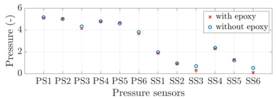
Figure 13.
Numerical pressure on the blade with and without epoxy.
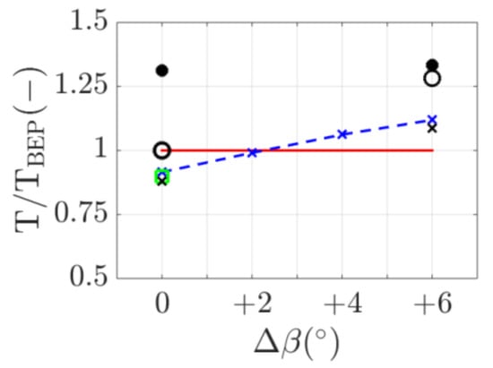
Figure 14.
Numerical scaled mean torque values at different runner blade positions and the experimental value. Results of the simulations at OP2. − experimental results; -x- steady-state simulations results; □ added epoxy simulation result; x unsteady upwind simulation results; ● unsteady high-resolution simulation results; and o unsteady high-resolution simulation results (complete runner domain).
4.3. Runner Blade Angle
The uncertainty of the experimental measurement on the runner blade angle could not be assessed. Therefore, a sensitivity analysis was performed to quantify the influence of the angle on the accuracy of the numerical simulations.
Figure 14 presents the variation of the non-dimensionalized torque values as a function of the runner blade angle increment. The steady simulations showed a linear increase of the torque as the runner was opened. The blade angle increased (see Figure 4), allowing for a larger lift and thus torque. The results of the unsteady simulations that included a single runner blade passage and employed the upwind advection scheme were similar to the results provided by the steady-state simulations. However, when the high-resolution advection scheme was used, the simulations showed a poor convergence of the monitored variables and the numerical torque values were strongly overestimated. The reason for the poor convergence is unclear but may be attributed to the periodic interfaces defined between the runner blade passages not accurately modelling the influence of the runner blade wakes in the turbulent flow. Including the complete runner geometry in the simulations lead to an improvement of the results of the simulation employing the experimental runner blade angle (Figure 14), and the numerical torque value matched surprisingly well the experimental value. However, at the larger runner blade angle, 6° more than the experimental value, the convergence of the monitored variables was impossible to achieve. The use of a very large blade angle while keeping the same total pressure at the inlet led to incoherent flow structures, large recirculation areas, and a negative flow rate.
Figure 15 presents the non-dimensionalized mean absolute pressure variation function of the runner blade angle. The pressure was monitored on both the pressure (from PS1 to PS6) and the suction side (from PS1 to PS6) of the same runner blade. The numerical and experimental pressure values were scaled with the reference pressure that was measured by Soltani et al. [1]. As the runner blade angle increased, i.e., the runner was opened, the absolute pressure monitored on the blade decreased. At the largest blade angle values, +4° and +6°, the pressure was strongly underestimated near the leading edge (PS4) and in the middle section (PS2) of the blade pressure side. The differences between the numerical results and the experimental data were reduced towards the trailing edge (PS3 and PS6). On the other hand, when using the experimental runner blade angle (Δβ = 0°), the numerical pressure values were in better agreement with the experimental values. The pressure was underestimated in the center area of the pressure side and near the leading edge (PS2 and PS4) but reasonably predicted near the trailing edge (PS3 and PS6). On the suction side of the blade, at the middle section, and near the trailing edge, the absolute pressure was overpredicted as the numerical simulation underestimated the hydraulic energy transferred to the runner.

Figure 15.
Numerical scaled mean absolute pressure values at different runner blade positions for the steady-state simulations at OP2. The dashed lines represent the experimental values measured at β = −4.2° (Δβ = 0°).
The experimentally determined runner blade angle, −4.2°, was employed in the definitive studies presented in the paper because the pressure measurements and the torque measurements best matched the experimental results.
4.4. Best Efficiency Point (OP2)
The numerical simulations presented in the following sections were unsteady simulations that included a single stay vane-guide vane passage, the complete runner domain and the draft tube. The cavitation model was employed. The runner blade angle was set at the experimental value, −4.2°, no clearances were considered, and the epoxy layer was not modelled.
4.4.1. Mean Values
The numerical mean torque value obtained was 109.7 kN·m, only 0.1% smaller than the experimental mean value of 109.8 kN·m. This result was presented in the previous section with the sensitivity analysis of the runner blade angle.
Figure 16 presents the experimental mean absolute pressure data measured on the runner blade and the pressure values obtained from the unsteady numerical simulation. The results were non-dimensionalized with the pressure value experimentally measured in the empty turbine chamber. The pressure variation was similar to the results provided by the steady-state simulations (Figure 15).
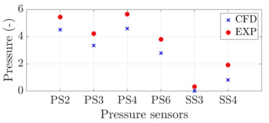
Figure 16.
Scaled mean absolute pressure values at OP2.
On the pressure side of the blade, the pressure was underestimated near the leading edge (PS4) and in the middle area (PS2). Towards the trailing edge, the numerical results showed a better match to the experimental data (PS3 and PS6), underestimating the pressure by less than 6%. The simulation overpredicted the pressure on the suction side near the trailing edge (SS3). Figure 17 and Figure 18 present iso-surfaces of the 20% vapor volume fraction captured at the end of the unsteady simulation after approximately three runner rotations. Towards the periphery of the runner blade suction side, the flow was accelerated and cavitation developed as pressure decreases. The flow was not axisymmetric, leading to larger cavitation areas near some blades and not others; see Figure 18.
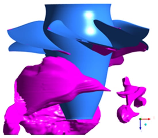
Figure 17.
Iso-surface of 20% vapor volume fraction at OP2 in the runner domain.
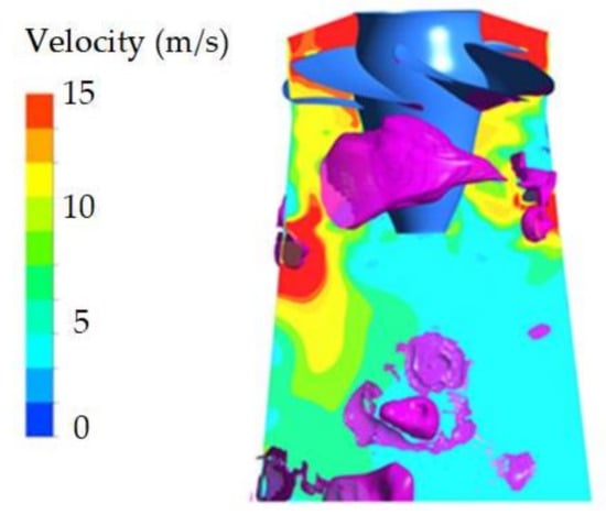
Figure 18.
Liquid water velocity in stationary frame and iso-surface of 20% vapor volume fraction at OP2 in the runner domain.
Figure 19 presents the wall shear stress variation on the suction side of the runner blades at OP2. The asymmetric flow was once again confirmed, leading to non-uniform flow separation on the suction side of the runner blades. The OP2 operating point was close to but not exactly the best efficiency point; therefore, it is possible that a vortex was beginning to form in the draft tube cone.
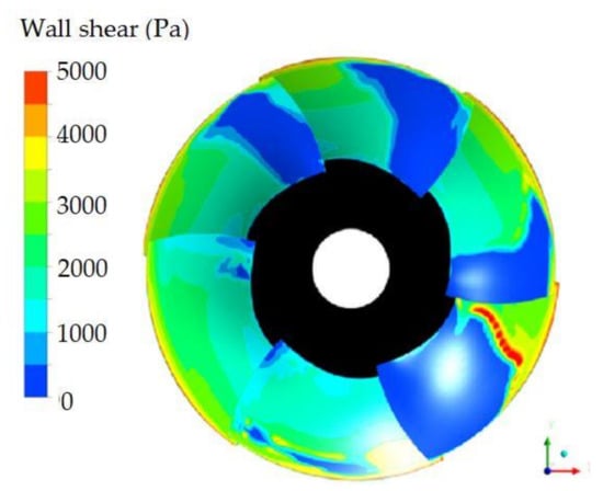
Figure 19.
Wall shear stress on the suction side of the runner blades at OP2.
4.4.2. Amplitude Spectrum Analysis
A fast Fourier transform (FFT) analysis was carried out to identify the frequency content of the numerical torque and pressure signals and to compare them to the experimental results. A single smooth area of the signal corresponding to one runner rotation was selected and added to itself to obtain a better resolution of the FFT. The torque was scaled by the mean torque value recorded at OP2 during the experimental measurements. The pressure was scaled by the reference pressure that was experimentally measured [1]. The mean values were subtracted from the numerical and the experimental signals. The lengths of the original signal and the analyzed signal were 0.1 and 110 s, respectively. The frequencies were non-dimensionalized (f*) using the runner frequency (fr) of 10 Hz.
Figure 20 presents the amplitude spectrum of the scaled torque for the numerical and experimental data. A factor of 5 was obtained between the amplitudes. The dimensionless frequency of 1, visible in the experimental data and corresponding to the runner frequency, was considered to be caused by the wake of the spiral casing lip junction [30]. In the numerical simulation, the spiral casing was not modelled but the same frequency was captured due to the multiplication of the signal corresponding to a single runner rotation. A second frequency peak at f* = 2 was captured in the experimental signal, though with a larger amplitude than the amplitude of the runner frequency, because two of the six runner blades were covered in epoxy. However, the peak at f* = 2 was visible in the simulations despite the epoxy layers not being modelled due to the selection of the signal to be analyzed (one runner rotation added to itself). The frequency peak at f* = 3.16 found in the experimental signals could represent a shaft torsional natural frequency. This may explain why the frequency was not present in the pressure measurements or the numerical torque.
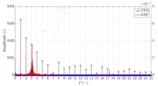
Figure 20.
Amplitude spectrum of the scaled torque at OP2. Two vertical axis are used, one for the experiments and one for the numerical results.
The dimensionless frequency of 2 was also visible in the amplitude spectrum of the experimental pressure signal (Figure 21). An additional peak was captured in the experiment at f* = 20, corresponding to the number of guide vanes, and not in the numerical results because only one guide vane-stay vane passage was modelled (Figure 5) with a stage interface.
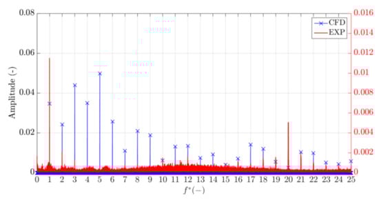
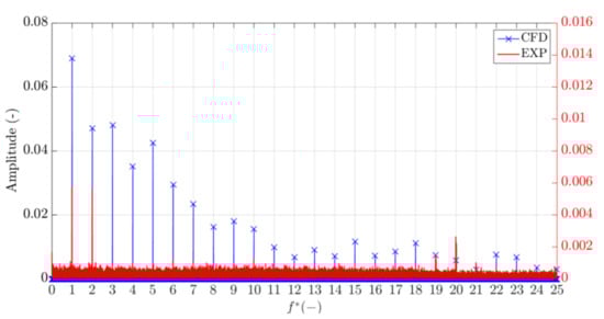
Figure 21.
Amplitude spectrum of the scaled pressure PS2 (top) and SS4 (bottom) at OP2. Two vertical axis are used, one for the experiments and one for the numerical results.
The numerical simulation could not capture all the experimental fluctuations, mainly because of the axial symmetry of the computational domain that did not include the spiral casing lip junction and the epoxy on the blade. However, the runner frequency and its harmonics were visible in the amplitude spectrum of the numerical torque and pressure, most likely because of the selection of a single runner rotation from the signal.
4.5. Part-Load Operation (OP1)
4.5.1. Mean Values
The numerical mean torque value obtained at OP1 was 71.5 kN·m. The numerical value was 8.3% smaller than the experimental mean value of 77.9 kN·m.
The dimensionless mean absolute pressure values obtained from the part-load (OP1) unsteady numerical simulation were compared to the experimental values shown in Figure 22. The numerical results followed the trend of the measured values and presented a good prediction of the pressure on the pressure side of the runner blade, with from 2.9 to 6.1% discrepancy compared with the experiment. The pressure was overestimated on the suction side along the blade span (SS4 and SS3) because the numerical simulation underestimated the fluid angular momentum transformed into torque.
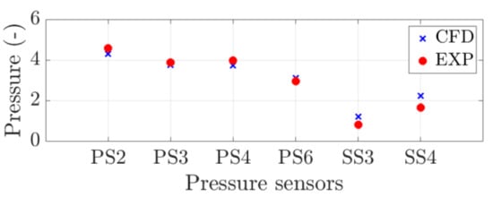
Figure 22.
Scaled mean absolute pressure values at OP1.
4.5.2. Amplitude Spectrum Analysis
At the part-load operation (OP1), the flow provided by the guide vanes has a high swirl. As a consequence, the tangential component of the velocity at the outlet of the Kaplan runner is larger, while the axial velocity is reduced [31]. The flow is pulled towards the draft tube walls, creating a low-pressure region below the runner cone in the center of the draft tube and leading to the formation of the RVR [32]. One complete RVR rotation corresponded to about six runner rotations in the present case. The dimensionless frequency of the RVR was found to be 0.17.
The pressure distribution and the velocity vectors in the runner and draft tube domains are presented in Figure 23. Low-pressure regions are visible below the runner cone (Figure 23a), and the corresponding recirculation zones were captured as the flow was concentrated near the draft tube walls (Figure 23b).

Figure 23.
(a) Mid-section pressure contour at OP1. (b) Velocity vectors.
Figure 24 presents iso-surfaces of the pressure in the draft tube. A double-helix vortex rope (left) was initially formed 3 s before the end of the numerical simulation. After 1.5 s, or 15 runner rotations, a single RVR was captured (middle) and remained so until the last time step (right).
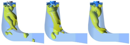
Figure 24.
Iso-surface at a constant pressure of 2 bar at OP1. Evolution of the RVR at 1.5 s intervals.
In the stationary reference frame of the draft tube, the RVR can be decomposed into two components [33] from two pressure measurements obtained at the same height and opposite to each other: the plunging and rotating modes. The plunging mode is associated with synchronous pressure pulsations recorded throughout the turbine. The rotating mode leads to pressure oscillations with the same frequency as the plunging mode.
Figure 25 presents the frequency spectrum of the numerical and experimental torque signals. The numerical data analyzed in the following section were obtained from the last 30 simulated runner rotations (10,800 time steps after convergence, or 3 s), i.e., 6 RVR rotations. The numerical simulation captured a frequency peak at f* = 0.17 matching the RVR dimensionless experimental frequency value of 0.17. Similar values were obtained during the measurement campaign of the Porjus U9 model and numerical studies investigating the Kaplan turbine model [10,23]. As the experimental and numerical data were obtained in the rotating domain, the amplitude at this frequency represents the plunging component. The RVR frequency is expected to show a slight variation at different part-load operating regimes [1]. The dimensionless frequency value of 0.83 corresponded to the rotating component of the RVR. It is visible in the experimental data because the blades were not identical and it was not captured by the numerical simulation.
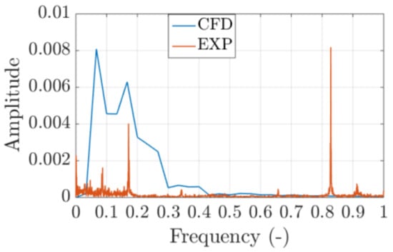
Figure 25.
Amplitude spectrum of the scaled torque at OP1.
On the pressure side of the runner blade, at PS4 near the leading edge and PS3 near the trailing edge, the plunging mode of the RVR represented by the peak at f* = 0.17 in the experimental data could also be found in the numerical results at the dimensionless frequency of 0.17 (Figure 26), similar to the torque FFT analysis. The amplitude was underestimated by the numerical model, especially closer to the leading edge (PS4). The rotating component of the RVR, 0.83 dimensionless frequency in the experiments, was captured in the numerical simulation at both locations of the pressure monitor points.
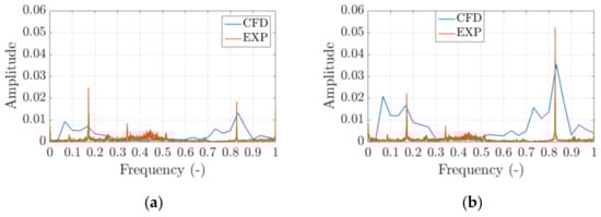
Figure 26.
Amplitude spectrum of the scaled pressure at OP1: (a) PS4 and (b) PS3.
Despite the overestimation of the mean absolute pressure values in the numerical studies on the suction side of the blade (Figure 22), the amplitude of the pressure fluctuations was in a better agreement with the experimental data (Figure 27). The numerical dimensionless frequencies of the plunging and rotating components of the RVR on the blade suction side were coherent with the values obtained in the experiment.
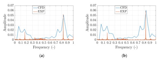
Figure 27.
Amplitude spectrum of the scaled pressure at OP1: (a) SS4 and (b) SS3.
4.6. RVR Decomposition
Two pressure monitor points diametrically opposed (Figure 5), DTin on the inner radius of the draft tube and DTout on the outer radius of the draft tube defined just below the runner cone in the numerical model, were selected for the decomposition of the RVR [33]. The amplitude of the plunging (Ppl) and rotating (Prot) modes was calculated as:
The two peaks were identified at the dimensionless frequency of 0.17, which was in good agreement with the FFT analysis of the torque and pressure signals (Figure 28). The amplitude of the pressure fluctuations due to the rotating component of the RVR was 30% smaller than the amplitude of the plunging mode. In the frequency spectrum of the plunging component, there were two additional frequency peaks at 0.1 and 0.23 m while in the frequency spectrum of the rotating component there are two peaks at 0.23 and 0.4 dimensionless frequencies. A possible explanation for these frequency peaks could be spectral leaking [34]. As the first and last values of the signal chosen for the analysis were not identical, high frequencies that were aliased between 0 and half of the sampling frequency may have “leaked” their energy into the other frequencies.
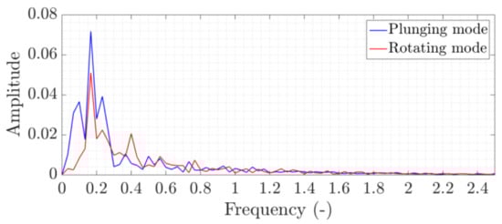
Figure 28.
RVR decomposition: plunging and rotating mode.
5. Conclusions
A numerical study of the Porjus U9 Kaplan prototype was carried out. Two operating points on a propeller curve, corresponding to the best efficiency point and part-load operating conditions, were modelled. The effects of the boundary conditions, runner blade clearance, blade geometry and mesh size on the numerical results were first investigated at the best efficiency point to minimize the computational efforts. Then, experimental pressure and torque measurements performed on the prototype were used to validate the numerical results.
Modelling the runner blade clearances and the epoxy layer added to the instrumented runner blade had no significant influence on the numerical results considering the increased mesh size and simulation time, so these parameters could be neglected.
The runner blade angle is a parameter that is challenging to measure on a turbine prototype. However, a parametric study showed that the runner blade angle strongly influences both the convergence and accuracy of numerical results.
The simplified model reasonably predicted the mean torque and pressure values at both operating points.
The steady simulations with a single runner passage and unsteady simulations at BEP provided similar results. Modelling the complete runner domain and including the cavitation model improved the convergence of the simulations and the mean torque prediction. However, the mean unsteady numerical pressure values were similar to the values obtained from the steady simulations. Therefore, steady single-passage simulations at BEP are an excellent first approximation.
At part-load operation, the numerical simulations captured the variation in the pressure due to the RVR observed in the experiment. The frequency of the pressure fluctuations was well-predicted both in the runner and the draft tube considering the simplified, axisymmetric computational domain. In the runner domain, the frequencies of the plunging and rotating components of the RVR were accurately determined by the simulation, except for the torque missing the RVR rotating component. The amplitudes of these pressure fluctuations were also reasonably predicted, especially on the suction side of the runner blade.
The spectral analysis of the numerical signals was strongly influenced by the convergence of the monitored numerical values and the signal selection to be analyzed. Due to the signal selection, the FFT analysis could have been altered by spectral leakage, leading to pressure peaks with no experimental correspondents.
Author Contributions
Conceptualization, M.J.C.; Formal analysis, M.J.C.; Investigation, R.G.I., A.S.D. and M.J.C.; Methodology, M.J.C.; Supervision, D.M.B. and M.J.C.; Writing—original draft, R.G.I.; Writing—review and editing, A.S.D., D.M.B. and M.J.C. All authors have read and agreed to the published version of the manuscript.
Funding
The European Union’s Horizon 2020 research and innovation program under grant agreement No. 814958 partially financed the research.
Institutional Review Board Statement
Not applicable.
Informed Consent Statement
Not applicable.
Data Availability Statement
Not applicable.
Acknowledgments
The presented research was carried out as a part of the Swedish Hydropower Centre (SVC), which was established by the Swedish Energy Agency, Elforsk and Svenska Kraftnät, together with the Luleå University of Technology, The Royal Institute of Technology, Chalmers University of Technology, and Uppsala University.
Conflicts of Interest
The authors declare no conflict of interest.
Abbreviations
| CtClr | constant clearance |
| DTin | numerical pressure recorded on the draft tube wall (inner radius) |
| DTout | numerical pressure recorded on the draft tube wall (outer radius) |
| f* | dimensionless frequency |
| FFT | Fast Fourier transform |
| fr | runner frequency |
| Hgross | gross head of the turbine |
| k | kinetic energy |
| LE | leading edge |
| NoClr | no clearance |
| OP1 and OP2 | operating points |
| Pout | power output |
| Ppl | plunging mode pressure |
| Prot | rotating mode pressure |
| RVR | rotating vortex rope |
| SST | Shear Stress Transport |
| TE | trailing edge |
| VarClr | variable clearance |
| y+ | dimensionless distance from the wall |
| z | elevation |
| β | runner blade angle |
| pressure drop obtained between the inlet and the outlet of the numerical domain | |
| νt | turbulent viscosity |
| ω | turbulent frequency |
References
- Soltani Dehkharqani, A.; Engstrom, F.; Aidanpää, J.O.; Cervantes, M.J. Experimental investigation of a 10 MW prototype axial turbine runner: Vortex rope formation and mitigation. J. Fluids Eng. 2020, 142, 101212. [Google Scholar] [CrossRef]
- Trivedi, C.H.; Gandhi, B.; Cervantes, M.J. Effect of transients on Francis turbine runner life: A review. J. Hydraul. Res. 2013, 51, 121–132. [Google Scholar] [CrossRef]
- Farhat, M.; Natal, S.; Avellan, F.; Paquet, F.; Couston, M. Onboard measurements of pressure and strain fluctuations in a model of low head Francis turbine—Part 1: Instrumentation. In Proceedings of the 21st IAHR Symposium on Hydraulic Machinery and Systems, Lausanne, Switzerland, 9–12 September 2002. [Google Scholar]
- Lowys, P.; Paquet, F.; Couston, M.; Farhat, M.; Natal, S.; Avellan, F. Onboard measurements of pressure and strain fluctuations in a model of low head Francis turbine—Part 2: Measurements and preliminary analysis results. In Proceedings of the 21st IAHR Symposium on Hydraulic Machinery and Systems, Lausanne, Switzerland, 9–12 September 2002. [Google Scholar]
- Cervantes, M.J.; Trivedi, C.H.; Dahlhaug, O.G.; Nielsen, T.K. Francis-99 workshop 1: Steady operation of Francis turbines. J. Phys. Conf. Ser. 2015, 579, 011001. [Google Scholar] [CrossRef] [Green Version]
- Trivedi, C.H.; Dahlhaug, O.G.; Selbo Storli, P.T.; Nielsen, T.K. Francis-99 workshop 3: Fluid structure interaction. J. Phys. Conf. Ser. 2019, 1296, 011001. [Google Scholar] [CrossRef]
- Vuillemard, J.; Aeschlimann, V.; Fraser, R.; Lemay, S.; Deschênes, C. Experimental investigation of the draft tube inlet flow of a bulb turbine. IOP Conf. Ser. Earth Environ. Sci. 2014, 22, 032010. [Google Scholar] [CrossRef] [Green Version]
- Fraser, R.; Coulaud, M.; Aeschlimann, V.; Lemay, J.; Deschênes, C. Method for experimental investigation of transient operation on Laval test stand for model size turbines. IOP Conf. Ser. Earth Environ. Sci. 2016, 49, 062006. [Google Scholar] [CrossRef] [Green Version]
- Mulu, B.G.; Cervantes, M.J. Experimental investigation of a Kaplan model with LDA. In Proceedings of the Water Engineering for Sustainable Environment: 33rd IAHR Congress, Vancouver, BC, Canada, 9–14 August 2009. [Google Scholar]
- Amiri, K.; Mulu, B.G.; Raisee, M.; Cervantes, M.J. Unsteady pressure measurements on the runner of a Kaplan turbine during load acceptance and load rejection. J. Hydraul. Res. 2016, 54, 56–73. [Google Scholar] [CrossRef]
- Trivedi, C.H.; Gogstad, P.J.; Dahlhaug, O.G. Investigation of the unsteady pressure pulsations in the prototype Francis turbines during load variation and startup. Renew. Sustain. Energy Rev. 2017, 9, 064502. [Google Scholar] [CrossRef]
- Unterluggauer, J.; Sulzgruber, V.; Doujak, E.; Bauer, C. Experimental and numerical study of a prototype Francis turbine startup. Renew. Energy 2020, 157, 1212–1221. [Google Scholar] [CrossRef]
- Wang, F.; Li, X.; Min, Y.; Ma, J. Experimental investigation of characteristic frequency in unsteady hydraulic behavior of a large hydraulic turbine. J. Hydrodyn. 2009, 21, 12–19. [Google Scholar] [CrossRef]
- Trivedi, C.H.; Gogstad, P.J.; Dahlhaug, O.G. Investigation of the unsteady pressure pulsations in the prototype Francis turbines–part 1: Steady state operating conditions. Mech. Syst. Signal Process. 2018, 108, 188–202. [Google Scholar] [CrossRef] [Green Version]
- Gagnon, M.; Jobidon, N.; Lawrence, M. Optimization of turbine startup: Some experimental results from a propeller runner. IOP Conf. Ser. Earth Environ. Sci. 2014, 22, 032022. [Google Scholar] [CrossRef]
- Presas, A.; Luo, Y.; Guo, B.; Wang, Z. Fatigue life estimation of Francis turbines based on experimental strain measurements: Review of the actual data and future trends. Renew. Sustain. Energy Rev. 2019, 102, 96–110. [Google Scholar] [CrossRef]
- You, F.; Sun, L. Machine learning and data-driven techniques for the control of smart power generation systems: An uncertainty handling perspective. Engineering 2021, 7, 1239–1247. [Google Scholar] [CrossRef]
- Bordin, C.; Skjelbred, H.I.; Kong, J.; Yang, Z. Machine learning for hydropower scheduling: State of the art and future research directions. Procedia Comput. Sci. 2020, 176, 1659–1668. [Google Scholar] [CrossRef]
- Huang, X.; Chamberland-Lauzon, J.; Oram, C.; Klopfer, A.; Ruchonnet, N. Fatigue analyses of the prototype Francis runners based on site measurements and simulations. IOP Conf. Ser. Earth Environ. Sci. 2014, 22, 012014. [Google Scholar] [CrossRef] [Green Version]
- Mössinger, P.; Jung, A. Transient two-phase CFD simulation of overload operating conditions and load rejection in a prototype sized Francis turbine. IOP Conf. Ser. Earth Environ. Sci. 2016, 49, 092003. [Google Scholar] [CrossRef]
- Karlsson, M.; Nilsson, H.; Aidanpää, J.O. Influence of inlet boundary conditions in the prediction of rotor dynamic forces and moments for a hydraulic turbine using CFD. In Proceedings of the 12th International Symposium on Transport Phenomena and Dynamics of Rotating Machinery, Honolulu, HI, USA, 17–22 February 2008. [Google Scholar]
- Mössinger, P.; Jester-Zürker, R.; Jung, A. Francis-99: Transient CFD simulation of load changes and turbine shutdown in a model sized high-head Francis turbine. J. Phys. Conf. Ser. 2017, 782, 012001. [Google Scholar] [CrossRef] [Green Version]
- Iovănel, R.G.; Dunca, G.; Bucur, D.M.; Cervantes, M.J. Numerical simulation of the flow in a Kaplan turbine model during transient operation from the best efficiency point to part load. Energies 2020, 13, 3129. [Google Scholar] [CrossRef]
- Tiwari, G.; Kumar, J.; Prasad, V.; Patel, V.K. Derivation of cavitation characteristics of a 3 MW prototype Francis turbine through numerical hydrodynamic analysis. Mater. Today Proc. 2020, 26, 1439–1448. [Google Scholar] [CrossRef]
- Li, D.; Song, Y.; Lin, S.; Wang, H.; Qin, Y.; Wei, X. Effect mechanism of cavitation on the hump characteristic of a pump-turbine. Renew. Energy 2021, 167, 369–383. [Google Scholar] [CrossRef]
- Hao, Y.; Tan, L. Symmetrical and unsymmetrical tip clearances on cavitation performance and radial force of a mixed flow pump as turbine at pump mode. Renew. Energy 2018, 127, 368–376. [Google Scholar] [CrossRef]
- Ansys® CFX, Release 16.2, Help System, Theory Guide; ANSYS, Inc.: Canonsburg, PA, USA, 2015.
- Joshi, A.; Assam, A.; Nived, M.R.; Eswaran, V. A Generalised wall function including compressibility and pressure-gradient terms for the Spalart–Allmaras turbulence model. J. Turbul. 2019, 20, 626–660. [Google Scholar] [CrossRef]
- Ansys® CFX, Release 16.2, Help System, Modelling Guide; ANSYS, Inc.: Canonsburg, PA, USA, 2015.
- Amiri, K.; Cervantes, M.J.; Mulu, B.G. Experimental investigation of the hydraulic loads on the runner of a Kaplan turbine model and the corresponding prototype. J. Hydraul. Res. 2015, 53, 452–465. [Google Scholar] [CrossRef]
- Wannassi, M.; Monnoyer, F. Numerical simulation of the flow through the blades of a swirl generator. Appl. Math. Model. 2016, 40, 1247–1259. [Google Scholar] [CrossRef]
- Sotoudeh, N.; Maddahian, R.; Cervantes, M.J. Investigation of rotating vortex rope formation during load variation in a Francis turbine draft tube. Renew. Energy 2020, 151, 238–254. [Google Scholar] [CrossRef]
- Bosioc, A.L.; Susan-Resiga, R.; Muntean, S.; Tanasa, C. Unsteady pressure analysis of a swirling flow with vortex rope and axial water injection in a discharge cone. J. Fluids Eng. 2012, 134, 1–11. [Google Scholar] [CrossRef]
- Lyon, D. The Discrete Fourier Transform, Part 4: Spectral Leakage. J. Object Technol. 2009, 8, 23–34. [Google Scholar] [CrossRef]
Publisher’s Note: MDPI stays neutral with regard to jurisdictional claims in published maps and institutional affiliations. |
© 2022 by the authors. Licensee MDPI, Basel, Switzerland. This article is an open access article distributed under the terms and conditions of the Creative Commons Attribution (CC BY) license (https://creativecommons.org/licenses/by/4.0/).