Abstract
Large-scale integration of PV generators in distribution grids will impair the voltage stability due to the stochastic and fluctuated PV power generation. To tame the volatile PV power generation, battery energy storage systems (BESS) are deployed as an effective yet expensive power buffering mechanism. In this paper, a dual ascent-based voltage optimization control is proposed to achieve the concurrent regulation of battery State-of-Charge (SoC), nodal voltages, and distribution loss. This control features the limited dependence on the communication network with information interaction between neighboring nodes. Besides, it can achieve the optimal power flow minimizing the distribution loss while maintaining the BESS SoC within a healthy range. The derivation of the control framework is provided, and comparative simulations in the IEEE 37-node distribution system are performed to validate the effectiveness of the proposed control algorithm.
1. Introduction
To decarbonize the energy system and prevent global warming, renewable energy sources, such as PV and wind power, are introduced as green alternatives to replace the fossil fuel energy sources in power systems. The power generation profile is highly associated with the solar irradiation condition and has a high uncertainty [1]. Considering the variable irradiance condition, the fluctuating PV powers will lead to grid overvoltage [2,3] and consequently result in PV deloading. This will degrade the energy efficiency of the PV.
To address the voltage issues and avoid PV deloading, many studies have been performed to buffer the fluctuated PV power and maintain the voltage stability in PV-integrated distribution grids, including PV inverter control [4,5], active and reactive power coordinative control of multiple PV generation units [6], modification of the characteristic curve of the overcurrent devices [7], model predictive and coordinative control [8], PV-battery coordinative control framework [9,10], etc. Among the reported methods, BESS can effectively reduce the voltage fluctuation without deloading the PV, which improves the PV hosting capacity of the distribution grids and received much research attention.
The control methods of BESS can be divided into conventional centralized control, decentralized control, and prevailing distributed control. In [9], a real-time centralized control scheme is reported to coordinate the voltage regulation efforts among the PV inverter and BESS. The centralized control scheme demands a central data processing and calculation unit for determining all the control commands [11,12], which suffers from high computation workload and requires a powerful communication infrastructure. The decentralized control schemes receive more attention as they effectively alleviate data exchange and calculation efforts, thus reducing the investments in the communication and calculation infrastructure [13,14]. Several studies have been performed on decentralized control schemes. An adaptive droop control scheme is reported in [15] to coordinate BESS for regulating nodal voltages in a PV-integrated low-voltage distribution network. A model-free data-driven multi-agent deep-reinforcement-learning decentralized control framework is reported in [16]. In this control scheme, the power profiles of both the static VAR compensators and BESSs are smoothened to control the voltages in distribution systems. In [17], a decentralized control scheme targeting the minimization of the generation cost, distribution loss, and voltage variation is reported. However, parts of the data process in decentralized control schemes still require centralized processing, limiting its dynamic performance. Therefore, the distributed control manner is needed due to its practicability, economy, and flexibility.
However, the current-voltage optimization control methods of AC distribution networks, based on distributed control architecture and BESS, are mostly lacking in pursuing optimal power flow or complete optimization goals. For example, a BESS distributed voltage regulation method based on a dynamic event-triggered mechanism is proposed in [18]. This method can effectively reduce the communication workload, but the optimization objective is unclear. Similarly, the BESS distributed consensus control method reported in [19] ignores the power flow optimization while solving the overvoltage/undervoltage cases in the distribution network. In addition, in [20], a BESS-based distributed voltage online optimization method is proposed. However, this method only focuses on voltage tracking and lacks a complete optimization objective design. Therefore, the distributed voltage optimization control method of the AC distribution network, which takes both distributed control and optimal power flow into account, is urgently needed.
A dual-ascent-based distributed voltage control scheme is proposed in this paper to regulate the voltages of the PV-integrated distribution grids and make full use of the BESS. The key contributions can be summarized as follows:
- (1)
- The distributed control scheme is adopted to solve this issue. The proposed method only requires the neighboring information to determine the optimal control commands, significantly reducing the computation and communication efforts. The control complexity is low, satisfying the real-time implementation requirement, which is suitable for a distributed PV generation system;
- (2)
- The optimal power flow is considered in the proposed method, making up for the deficiency of current research. Besides, the BESS cost is also minimized based on the objective function;
- (3)
- The convergence rate is given full consideration so that the proposed method can be implemented online. According to the simulation results, the convergence rate meets the requirement of the dynamic voltage support from different types of distributed energy resources [21].
The rest of this paper is organized as follows. Models, including communication network, BESS, and AC load flow, are introduced in Section 2. The optimization objective function and constraints are discussed in Section 3. The proposed distributed voltage control method is elaborated in Section 4. Simulation results of the proposed methods are provided in Section 5, and a conclusion is drawn in Section 6.
2. Materials and Methods
2.1. Distribution Grid and Communication Network Model
In this section, we consider a radial graph
. In
denotes the set of nodes with the first node defined as the root node, and ε represents the directed edges. Node j is defined as the neighbor of node i if there exists a directed edge with node i being the head and node j being the tail. Similarly, neighborhood node set of node i is defined as . The incidence matrix used in this paper is defined as [22]:
where A is an n × (n + 1) matrix with a rank of n.
When denotes the root node column, namely, the first column of , (1) can be rewritten as
where A is the rest of .
2.2. BESS Model
By applying the Coulomb counting method, the battery SoC at the time step of n + 1 can be calculated as
where , and denote the battery power, terminal voltage, and rate capacity of the i-th BESS. is the i-th battery SoC at the time step n. ΔT is the deviation between each time step. Considering the electrochemical feature of the battery, it is desirable to operate the battery SoC at the median of its maximum and minimum SoC, for example
where and are the supremum and infimum of the i-th battery SoC, and is the desirable reference of the i-th battery SoC. The battery SoC median will be used as the control reference in this paper.
2.3. AC Load Flow Model
For radial distributed networks, the AC load flow of a branch can be expressed by using [23]
where is the set of node i’s neighbors. is the voltage at node i. r and x denote the resistance and reactance of the distribution line, respectively. and are the active and reactive powers on line i sent from node . and are the sum of active and reactive power loads and injections at node , respectively. Details of and will be specified afterward.
The nodal voltage relationship between the sending node i and the receiving node j can be expressed as [23]
The AC load flow model is simplified by using the LinDistFlow mode to reduce calculation complexity. Considering the nodal voltage variations are insignificant, they are approximated as 1, that is, . Based on these simplifications and linearizations [24], the AC load flow model discussed above can be rewritten as
When the BESS and PV are considered, the nodal power flow can be expressed as
where and are the loads at node i. and are the PV power injections at node i. and are the BESS power injections at node i.
3. Formulation of the Optimization Model
3.1. Optimization Target
The voltage optimization control targets are (i) to minimize the distribution loss and (ii) to regulate the battery SoC in the vicinity of the median SoC. Typically, the distribution loss can be expressed as
where NG is the set of nodes in the distribution network.
To benefit the battery health and enable sufficient energy buffering capability, the BESS SoC shall be the median of its maximum and minimum SoC. In other words, BESS energy (E) shall be as close to the median as possible. Therefore, the BESS SoC cost function can be formulated as
where EF stands for the energy regulation efficiency, which is represented by the difference between the SoC and the desirable reference. Wi is the weighting factor of node i. The details of Wi will be specified afterwards. And is the desirable reference of the i-th BESS energy, which will be detailed afterwards. According to (3),
Therefore, according to (4), the desirable reference of the i-th BESS energy can be formulated as
The overall cost function can be obtained by calculating the weighted sum of the distribution loss and SoC loss
To put them in matrix form, the distribution loss can be rewritten as
where and are the diagonal matrices with their i-th diagonal elements being and , respectively. and are the column vectors composed of and , respectively.
By transferring (8) and (9) into the matrix form, it can be derived that
By transferring (19), (20) into (13), it can be derived that
where and .
Similarly, the SoC cost can be rearranged in matrix form as
By defining W = KR to normalize EF with respect to LS, it can be derived that
where K is a scalar.
Therefore, the final objective function can be expressed as
3.2. Constraints of the Load Flow
The matrix forms of the load flow equality constraints (5)–(7) can be expressed as
Similarly, the nodal voltage constraints can be rearranged in matrix form as
Generally, the nodal voltages must be operated within the range of [0.95 p.u., 1.05 p.u.].
3.3. Constraints of BESS
Considering the power capacity of the converter and battery, the power limit of the BESS can be expressed as
where is the rated apparent power of the BESS. In order to decouple the active and reactive power, the range of is linearized as . and are defined as and .
The BESS SoC limit can be expressed as
By substituting it into (15), it can be derived that
where , , , , , , , and are the lower bounds and upper bounds of BESS active power output, reactive power output, SoC, and battery energy at time step n + 1.
4. Distributed Voltage Control
The DA method is a distributed optimization algorithm. For the formulated optimization problem
Its Lagrangian function can be expressed as [22]
where , , are Lagrangian multipliers. and represent the upper and lower bounds of each multiplier.
The dual problem of (39), for example, , is the infimum of (39), which can be expressed as
As a result, the original problem can be transferred as
The original problem can be solved by following the steps below:
STEP 1: Obtain Lagrangian Multipliers. Solve the dual problem of the original problem so that the Lagrangian multiplier can be obtained.
According to the DA method, the iteration of the Lagrangian multiplier can be expressed as
where represents the gradient. LM is the column vector of the Lagrangian multipliers as . denotes the column vector of step sizes at the n-th iteration as .
Specifically, the updating process of the Lagrangian multiplier can be expressed as
STEP 2: Calculate the power reference. Substitute the Lagrangian multipliers into and solve the problem , and the reference BESS power and can be obtained.
By the DA method, the reference to be obtained can be expressed as
Considering is convex, and and are decoupled, its minimum will satisfy the condition of and .
Therefore, at the n-th iteration, the reference can be calculated in two parts:
PART 1: Calculation by local information.
PART 2: Calculation by communication with neighbors.
so that the reference BESS active power at the n-th iteration can be calculated by
5. Simulation Results
To validate the effectiveness of the proposed control algorithm, the control algorithm is implemented in a modified IEEE 37-bus system, as Figure 1 shows. In this system, fourteen distributed solar generation units and seven BESS are installed. The corresponding specifications can be summarized as shown in Table 1. In the simulation, the system is separately operated by the centralized control and the proposed distributed control schemes.
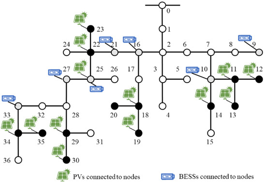
Figure 1.
The modified IEEE 37-bus system.

Table 1.
Parameters used in the simulation.
To systematically evaluate the control performance of the two-control scheme, both the static and dynamic operating conditions are simulated.
For the static case, both control schemes are applied to operate the system from a specific operating point towards the optimum. In the dynamic case, both control methods are implemented to dynamically regulate the system voltage under twenty-four-hour variable PV generation conditions. The applied solar power generation profile is shown in Figure 2.
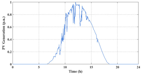
Figure 2.
The solar power generation profile.
All of the tests are implemented using MATLAB R2021a on a personal computer with an Intel Core i5 of 1.6 GHz and 8 GB memory.
5.1. Simulation Results of Static Case
In the static condition, the simulated time point is set at 12:00, and the load demand is configured to be 80% of the peak.
The change in the maximum and minimum system voltage with respect to the iterative steps can be plotted as shown in Figure 3. Figure 4 shows the convergence of the total distribution loss and cost with respect to the iterative process. As analyzed in [25], the theoretical convergence rate is . The computation time of 100 iterations is about 0.70 s, which is satisfied the system operation requirement [21]. Figure 5 shows the eventual nodal voltages of the system after the iteration process. When the proposed control is not applied, nearly 30% of the nodal voltages exceed the limits. However, the nodal voltage is within the safety requirement when the proposed control method is applied. This proves that the proposed control method can effectively operate the BESS to regulate the bus nodal voltage against the interruptive PV generation.
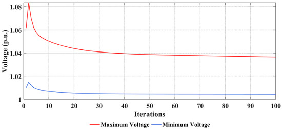
Figure 3.
Convergence of the maximum and minimum bus voltage magnitude.
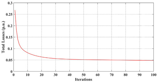
Figure 4.
Convergence of the total losses.
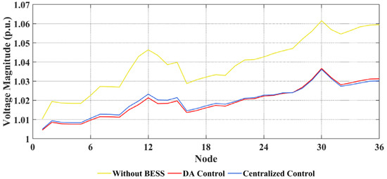
Figure 5.
Voltage Magnitude of Each Node under Three Scenarios.
The distribution loss of the system with the centralized/distributed control and without any control are summarized as shown in Table 2. In this table, Ploss is the distribution loss. Total Loss is the sum of the distribution loss and BESS regulation cost. The term ‘Ratio’ denotes the ratio between Total Loss and Ploss.
Table 2.
Total Losses among three scenarios.
By comparison, it can be concluded that (i) the engagement of the BESS can effectively minimize the distribution loss. (ii) The proposed distribution control scheme has a similar performance to the centralized method, which proves the effectiveness of the proposed methods. However, it is worth mentioning that the centralized control scheme is unlikely to achieve real-time implementation when the system is large, and the communication delay is significant.
5.2. Simulation Results of Dynamic Case
In this case, the PV generation is distributed in the system, and their generation profile can be shown in Figure 2. Meanwhile, the load profile also varies [26], as shown in Figure 6. The simulation is performed for 24 h. The neighboring nodes exchange information and update their local control reference every 1 min. The simulation is performed repetitively for three cases, including the case without BESS, the case with BESS under the centralized control scheme, and the case with BESS under the distributed control scheme.
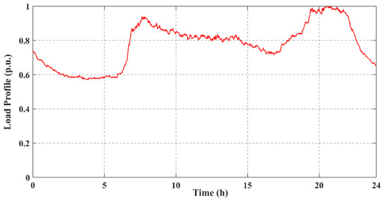
Figure 6.
The load profile.
To demonstrate the dynamic performance of the control algorithm, the 24 h maximum and minimum voltage magnitude profiles are plotted as shown in Figure 7 and Figure 8. Combined with the PV generation profile and load profile, it can be concluded that
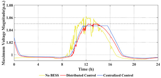
Figure 7.
Maximum voltage magnitude among a day.
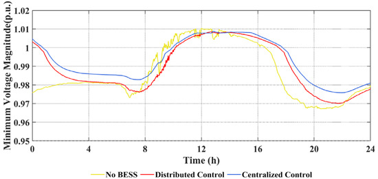
Figure 8.
Minimum voltage magnitude among a day.
- (i)
- When BESS is not installed, during the period of 11:00–14:00, the PV generation exceeds the load demand, and the nodal voltage surges and keeps exceeding the maximum for nearly 13% of the day. When BESS is installed, it can buffer the excessive PV power for regulating the nodal voltage within the safety range, proving the necessity of installing the BESS. Besides, the distributed control scheme can have nearly identical performance in bus voltage regulation compared with the centralized method;
- (ii)
- Comparing the control effect in Figure 7, the centralized control is better than the proposed algorithm when the voltage magnitude exceeds the limit (especially from 12:00 to 14:00). This is due to the inevitable convergence error of the distributed optimization method, the discussion of which can be found in [27]. The convergence error of each control period accumulates through the variable . Thus, it results in slight deviations under these two control structures. However, the difference is relatively small and is negligible for most control periods;
- (iii)
- Since the PV output throughout the day does not lead to undervoltage case, the minimum voltage curves in the three scenarios are similar. This performance is related to the choice of Lagrangian multipliers step (). When the voltage is within the acceptable range ([0.95 p.u., 1.05 p.u.]), the voltage-related multipliers step () is set to be small.
The network losses under three scenarios are shown in Figure 9. By comparison, it can be found that network loss of the cases with and without BESS is significantly different, especially when the PV generation is at the fastigium (10:00–15:00). When BESS is not involved, the maximum loss is up to 150 kW. When BESS is involved in the voltage regulation process, the power loss is much smaller. Compared to the case without BESS, the network loss is significantly reduced, with a maximum reduction in nearly 50%. This is due to the involvement of the BESS alleviating the overvoltage caused by the PV overgeneration. Moreover, the BESS effectively confines the voltage drop to the safe range, thus reducing the network loss.
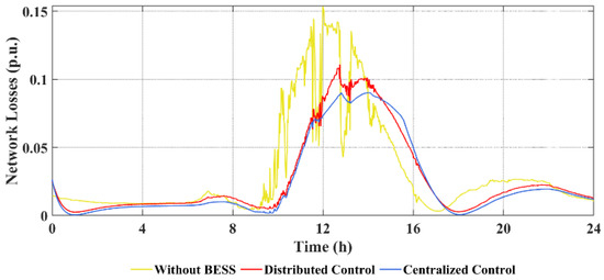
Figure 9.
Network Losses under three scenarios.
The BESS SoC daily profiles with centralized and proposed algorithms are shown in Figure 10 and Figure 11, respectively. The SoC difference between the two algorithms is shown in Figure 12. By comparison, it can be found that:
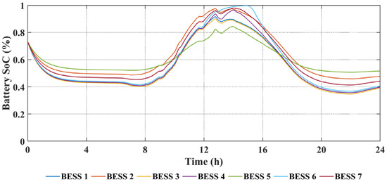
Figure 10.
Battery SoC under centralized control.
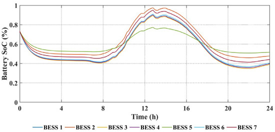
Figure 11.
Battery SoC under distributed control.
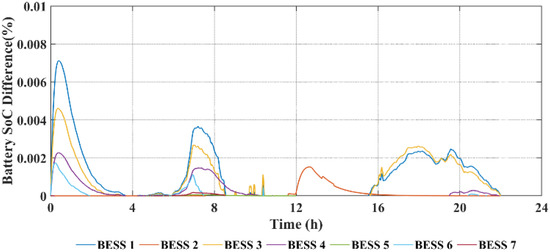
Figure 12.
Battery SoC difference between two algorithms.
- (i)
- The BESS SoC performance is similar under these two algorithms, which is consistent with the voltage performance, proving the effectiveness of the proposed algorithm. The reason for the tiny SoC difference between the two algorithms is mentioned above. This is due to the inevitable convergence error of the distributed optimization method;
- (ii)
- The output performance of each BESS is different. This is related to the BESS location. Since the options of the adjustment step () related to and are decided by R, the output sensitivity of each BESS is different so that there will be different output performance at the same time step.
The energy absorbed and released by BESS is shown in Figure 13. It can be found that the BESS energy profile and PV generation profile are consistent. When PV output is low, BESS releases energy. When PV output is high (9:00–15:00), BESS absorbs energy. This indicates that BESS plays a supporting role in the voltage maintenance under high PV penetration.
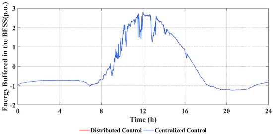
Figure 13.
Energy buffered in the BESS.
6. Conclusions
Due to the randomness and fluctuation of PV generation, high PV penetration may lead severe overvoltage issues to the distribution network. BESS is deployed and applied as an effective voltage fluctuation buffer mechanism to suppress the influence of PV generation on the distribution network. However, the related works so far have limited consideration on the optimal power flow and the regulating ability of the BESS.
In this paper, a distributed control scheme is proposed to operate BESS for regulating the voltages in PV-integrated distribution grids. The proposed control scheme features the concurrent functions of minimizing the distribution loss and manipulating BESS SoC. The dual ascent method is applied to solve the formulated optimization problem in a distributed manner.
The simulation results prove that the proposed control has a similar performance to the centralized control method. However, the proposed control method has a reduced requirement on the communication infrastructure, which is more viable in distribution systems.
The future work is expected to be carried out from the following aspects:
- (1)
- There are several theoretical studies on how to improve the convergence rate of DA algorithm. Distributed finite-time voltage optimization control method will be investigated based on these theoretical works;
- (2)
- The BESS-based distributed cooperative optimization control for frequency and voltage stability will be investigated to eliminate the effect of high PV penetration in the distribution network;
- (3)
- A hardware-in-loop real-time simulation platform will be established to verify the effectiveness of the proposed method in a laboratory scale.
Author Contributions
Conceptualization, Z.L. and Y.Y.; methodology, Z.L., Y.Y. and M.W.; writing—original draft preparation, Z.L.; writing—review and editing, Z.L., Y.Y., D.Q., S.Y. and M.W.; supervision, D.Q. and M.W. All authors have read and agreed to the published version of the manuscript.
Funding
This research was funded in part by the National Natural Science Foundation of China (No. U1909201) and in part by the Environment and Conservation Fund & Woo Wheelock Green Fund (ECF 108/2021).
Institutional Review Board Statement
Not applicable.
Informed Consent Statement
Not applicable.
Data Availability Statement
Not applicable.
Conflicts of Interest
The authors declare no conflict of interest.
References
- Ji, H.; Wang, C.; Li, P.; Ding, F.; Wu, J. Robust Operation of Soft Open Points in Active Distribution Networks with High Penetration of Photovoltaic Integration. IEEE Trans. Sustain. Energy 2018, 10, 280–289. [Google Scholar] [CrossRef]
- Huang, X.; Liu, H.; Zhang, B.; Wang, J.; Xu, X. Research on local voltage control strategy based on high-penetration distributed PV systems. J. Eng. 2019, 2019, 5044–5048. [Google Scholar] [CrossRef]
- Janiga, K. A review of voltage control strategies for low-voltage networks with high penetration of distributed generation. Inform. Autom. Pomiary W Gospod. I Ochr. Sr. 2020, 10, 61–65. [Google Scholar] [CrossRef]
- Ku, T.-T.; Lin, C.-H.; Chen, C.-S.; Hsu, C.-T. Coordination of transformer on-load tap changer and PV smart inverters for voltage control of distribution feeders. IEEE Trans. Ind. Appl. 2018, 55, 256–264. [Google Scholar] [CrossRef]
- Liu, J.; Li, Y.; Rehtanz, C.; Cao, Y.; Qiao, X.; Lin, G.; Song, Y.; Sun, C. An OLTC-inverter coordinated voltage regulation method for distribution network with high penetration of PV generations. Int. J. Electr. Power Energy Syst. 2019, 113, 991–1001. [Google Scholar] [CrossRef]
- Chai, Y.; Guo, L.; Wang, C.; Zhao, Z.; Du, X.; Pan, J. Network Partition and Voltage Coordination Control for Distribution Networks with High Penetration of Distributed PV Units. IEEE Trans. Power Syst. 2018, 33, 3396–3407. [Google Scholar] [CrossRef]
- Fani, B.; Bisheh, H.; Sadeghkhani, I. Protection coordination scheme for distribution networks with high penetration of photovoltaic generators. IET Gener. Transm. Distrib. 2018, 12, 1802–1814. [Google Scholar] [CrossRef]
- Mahdavi, S.; Panamtash, H.; Dimitrovski, A.; Zhou, Q. Predictive Coordinated and Cooperative Voltage Control for Systems with High Penetration of PV. IEEE Trans. Ind. Appl. 2021, 57, 2212–2222. [Google Scholar] [CrossRef]
- Wang, L.; Bai, F.; Yan, R.; Saha, T.K. Real-time coordinated voltage control of PV Inverters and energy storage for weak networks with high PV penetration. IEEE Trans. Power Syst. 2018, 33, 3383–3395. [Google Scholar] [CrossRef] [Green Version]
- Tewari, T.; Mohapatra, A.; Anand, S. Coordinated Control of OLTC and Energy Storage for Voltage Regulation in Distribution Network with High PV Penetration. IEEE Trans. Sustain. Energy 2020, 12, 262–272. [Google Scholar] [CrossRef]
- Unigwe, O.; Okekunle, D.; Kiprakis, A. Smart coordination of battery energy storage systems for volt-age control in distribution networks with high penetration of photovoltaics. J. Eng. 2019, 2019, 4738–4742. [Google Scholar] [CrossRef]
- Al-Saffar, M.; Musilek, P. Reinforcement learning-based distributed BESS management for mitigating over-voltage issues in systems with high PV penetration. IEEE Trans. Smart Grid 2020, 11, 2980–2994. [Google Scholar] [CrossRef]
- Suresh, V.; Pachauri, N.; Vigneysh, T. Decentralized control strategy for fuel cell/PV/BESS based microgrid using modified fractional order PI controller. Int. J. Hydrog. Energy 2020, 46, 4417–4436. [Google Scholar] [CrossRef]
- Vazquez, N.; Yu, S.S.; Chau, T.K.; Fernando, T.; Iu, H.H.C. A fully decentralized adaptive droop optimization strategy for power loss minimization in microgrids with PV-BESS. IEEE Trans. Energy Convers. 2018, 34, 385–395. [Google Scholar] [CrossRef]
- Jamroen, C.; Pannawan, A.; Sirisukprasert, S. Battery energy storage system control for voltage regulation in microgrid with high penetration of PV generation. In Proceedings of the 2018 53rd International Universities Power Engineering Conference (UPEC), Glasgow, UK, 4–7 September 2018; pp. 1–6. [Google Scholar] [CrossRef]
- Cao, D.; Zhao, J.; Hu, W.; Ding, F.; Huang, Q.; Chen, Z.; Blaabjerg, F. Data-driven multi-agent deep reinforcement learning for distribution system decentralized voltage control with high penetration of PVs. IEEE Trans. Smart Grid 2021, 12, 4137–4150. [Google Scholar] [CrossRef]
- Zhuang, P.; Liang, H. Hierarchical and Decentralized Stochastic Energy Management for Smart Distribution Systems with High BESS Penetration. IEEE Trans. Smart Grid 2019, 10, 6516–6527. [Google Scholar] [CrossRef]
- Kang, W.; Chen, M.; Guan, Y.; Wei, B.; Guerrero, J.M. Event-triggered distributed voltage regulation by heterogeneous BESS in low-voltage distribution networks. Appl. Energy 2022, 312, 118597. [Google Scholar] [CrossRef]
- Zeraati, M.; Golshan, M.E.H.; Guerrero, J.M. Distributed control of battery energy storage systems for voltage regulation in distribution networks with high PV penetration. IEEE Trans. Smart Grid 2018, 9, 3582–3593. [Google Scholar] [CrossRef] [Green Version]
- Zhao, T.; Parisio, A.; Milanović, J.V. Distributed control of battery energy storage systems in distri-bution networks for voltage regulation at transmission–distribution network interconnection points. Control. Eng. Pract. 2022, 119, 104988. [Google Scholar] [CrossRef]
- NationalgridESO. Power Potential DER Technical Requirements v2.5.3. 2019. Available online: https://www.nationalgrideso.com/document/114901/download (accessed on 29 May 2022).
- Li, J.; Xu, Z.; Zhao, J.; Zhang, C. Distributed Online Voltage Control in Active Distribution Networks Considering PV Curtailment. IEEE Trans. Ind. Inform. 2019, 15, 5519–5530. [Google Scholar] [CrossRef]
- Baran, M.E.; Wu, F.F. Network reconfiguration in distribution systems for loss reduction and load balancing. IEEE Power Eng. Rev. 1989, 9, 101–102. [Google Scholar] [CrossRef]
- Baran, M.; Wu, F. Optimal sizing of capacitors placed on a radial distribution system. IEEE Trans. Power Deliv. 1989, 4, 735–743. [Google Scholar] [CrossRef]
- Lin, Y.; Shames, I.; Nesic, D. Asynchronous distributed optimization via dual decomposition and block coordinate ascent. In Proceedings of the 2019 IEEE 58th Conference on Decision and Control (CDC), Nice, France, 11–13 December 2019; pp. 6380–6385. [Google Scholar] [CrossRef]
- Georges, H.; Alice, B. Individual Household Electric Power Consumption Data Set. UCI Machine Learning Repository. 2012. Available online: http://archive.ics.uci.edu/ml/datasets/Individual+household+electric+power+consumption (accessed on 30 May 2022).
- Boyd, S.; Xiao, L.; Mutapcic, A. Subgradient Methods. 2003. Available online: https://info.usherbrooke.ca/jpdussault/ROP771H17/subgrad_method_notes.pdf (accessed on 30 May 2022).
Publisher’s Note: MDPI stays neutral with regard to jurisdictional claims in published maps and institutional affiliations. |
© 2022 by the authors. Licensee MDPI, Basel, Switzerland. This article is an open access article distributed under the terms and conditions of the Creative Commons Attribution (CC BY) license (https://creativecommons.org/licenses/by/4.0/).