Article

Structural Optimization of Jet Fish Pump Design Based on a Multi-Objective Genetic Algorithm

1
College of Energy Engineering, Zhejiang University, Hangzhou 310027, China
2
College of Metrology and Measurement Engineering, China Jiliang University, Hangzhou 310018, China
3
Zhejiang Nanyuan Pump Industry Co., Ltd., Huzhou 313219, China
4
School of Mechanical Engineering, Zhejiang University of Technology, Hangzhou 310014, China
5
Zhijiang College, Zhejiang University of Technology, Hangzhou 310024, China
*
Authors to whom correspondence should be addressed.
Energies 2022, 15(11), 4104; https://doi.org/10.3390/en15114104
Submission received: 5 May 2022 / Revised: 30 May 2022 / Accepted: 31 May 2022 / Published: 2 June 2022
(This article belongs to the Special Issue Key Technologies and Challenges of Hydraulic Machinery and Systems)

Abstract

:
Jet fish pumps are efficient hydraulic machinery for fish transportation. Yet, the complex flow phenomenon in it is the major potential risk for damage to fish. The dangerous flow phenomena for fish, such as radial pressure gradient and exposure strain rate, are usually controlled by the structural parameters of jet fish pumps. Therefore, the injury rate of fish can be theoretically decreased by the structural optimization design of jet fish pumps. However, there is a complex nonlinear relation between flow phenomena and key structural parameters. To solve this problem, the present paper established a complex mapping between flow phenomena and structural parameters, based on computational fluid dynamics and a back-propagation neural network. According to this mapping, an NSGA-II multi-objective genetic algorithm was used to optimize the structure of jet fish pumps. The results showed that the optimized jet fish pumps could reduce the internal radial pressure gradient, exposure strain rate and danger zone to 40%, 12.5% and 50% of the pre-optimization level, respectively. Therefore, the optimized jet fish pump could significantly reduce the risk of fish injuries and keep the pump efficiency at a high level. The results could provide a certain reference for relevant structural optimization problems.

1. Introduction

In 2020, the Food and Agriculture Organization of the United Nations (FAO) pointed out that the world’s capture fisheries and aquaculture production have shown a rising trend in the past 80 years, and how to efficiently transport fish has become a key to fetching fish [1]. Therefore, there is a need for fish pumps capable of effectively carrying out live fish catching work, to replace the traditional fish transportation method. According to the working principle, fish pumps can be generally divided into vacuum fish pumps, centrifugal fish pumps, air-lift fish pumps and jet fish pumps [2]. The vacuum fish pump sucks and discharges the fish water mixture through negative vacuum pressure. Although resulting in slight fish loss, its intermittent suction and discharge work methods lead to low efficiency and high power consumption [3]. Centrifugal fish pumps are divided into submersible and fixed types depending on the installation position. They rely on the centrifugal force induced by the specially designed high-speed rotating impeller to suck the fish and water mixture, but this working principle causes a high damage rate to fish [4]. Air-lift fish pumps first use a blower to generate negative pressure in a pipe. When the wind speed in the tube is greater than the suspension speed of the fish, fish are sucked into the fish pump. The fish loss is modest, but the efficiency is low [5]. The jet fish pump is a particular type of annular jet pump that utilizes high-speed annular jet flow to entrain a mixture flow of water and fish, and it can continuously transport a variety of fish [6]. The structure of the jet fish pump is simple without any rotating impellers, so the mechanical damage risk for fish is relatively low. Therefore, compared with other fish pumps, jet fish pumps have better performance for live fish transportation.
Jet fish pumps were firstly used in the United States as early as 1922. Yet, it was not until recent decades that scholars paid attention to the research on jet fish pumps. The preliminary research studied the design of jet fish pumps affected by structural parameters, for example, the throat [7]. After that, following studies focused on the fish in jet fish pumps. Xiao et al. [3] used a high-speed camera to record the fish locomotion characteristics in a jet fish pump and theoretically analyzed the force on fish. According to this experiment, the team of Long [2] numerically studied the internal flow of jet fish pumps and discussed potential risks for fish injuries. In the same year, Wu et al. [8] experimentally studied changes in blood indexes to obtain the stress response of grass carp after passing through jet fish pumps. A year later, Xu et al. [6] conducted a series of experiments to research the transport capacity of jet fish pumps for different kinds of fish and their diversities of physiological changes were analyzed. Due to the irregular movement of fish in jet fish pumps, the experiment was the main method to study the locomotion of stressed fish before 2018. In 2019, Xu et al. [9] made a significant step toward the numerical simulation of stressed fish locomotion, developing an image-based numerical simulation method to study the locomotion of fish in jet fish pumps. Based on this method, rich flow details could be obtained, including the distribution of pressure and velocity around fish.
Yet, the working principle of jet fish pumps causes several unavoidable complicated hydraulic factors; shear flow and pressure gradient are typical injury risk sources for fish. Experiments are the common research method to study shear flow. By exposing the fish to a submerged jet, Neitzel et al. [10] studied the effect of shear flows on various types of juvenile fish and introduced a strain rate as an index of the shear intensity to describe the hydraulic force experienced by a fish in the shear environment. They [11] found that different fish species had different sensitivities to strain rate and fish could be damaged when strain rates were more than 500 s−1. Guensch et al. [12] checked the effects of shear flows and found that eye injuries and operculum injuries were common. Pressure gradients including compression and decompression are common hydraulic factors. Rapid decompression is dangerous for fish because it can cause barotrauma [13]. Typical symptoms of barotrauma include exophthalmia, protrusions of the everted stomach and gonads, overexpansion or rupture of the swim bladder, displacement of internal organs and rupturing of blood vessels and kidneys [14]. Some fish have even been killed by the barotrauma in the process of decompression [15]. Therefore, these dangerous hydraulic factors should merit more attention. Xu et al. [16,17] numerically studied the effects of pressure gradients and shear flow on fish and revealed the mechanism of fish external damage caused by these hydraulic factors. These hydraulic factors are the root of fish injury and are mainly determined by structural parameters. Thus, further research on jet fish pumps relies on the optimization of fish injury and transportation performance. For optimization, the biggest challenge lies in the nonlinear relationship between hydraulic factors and structural parameters. Additionally, the change of structural parameters also affects the efficiency and transportation performance of jet fish pumps. Therefore, it is a multi-parameter and multi-objective optimization problem aiming at high pump efficiency and low fish loss.
It is hard to directly establish this nonlinear relationship using traditional methods, so an advanced optimization method is needed. Currently, BP (back-propagation) neural network technology is a good choice to develop complex relationships between multiple objectives [18]. A BP neural network was considered with arbitrarily complex pattern classification capabilities and excellent multi-dimensional function mapping capabilities [19]. This technology does not need to determine the mathematical equation of the mapping relationship between input and output in advance. It only learns some rules through its own training and obtains the result closest to the expected output value when the input value is given. As for multi-objective optimization, evolutionary algorithms such as NSGA-II have become the main method for multi-objective optimization problems currently [20]. NSGA-II is a non-dominated sorting genetic algorithm with an elite strategy [21]. NSGA-II uses crowdedness and crowdedness comparison operators to make the individuals in the Pareto domain evenly distributed in the entire Pareto domain [22].
In this research, the flow characteristics in jet fish pumps with different structural parameters were numerically studied. After that, corresponding fish damage was evaluated, according to hydrodynamic theory and multi-objective optimization theory. The BP neural network was used to establish the internal mapping between structural parameters and fish damage. Aiming at reducing fish loss while keeping efficiency without significant decrease, an NSGA-II multi-objective genetic algorithm was used to solve this mapping relationship and the optimized structural parameters of the jet fish pump were obtained.

2. Materials and Methods
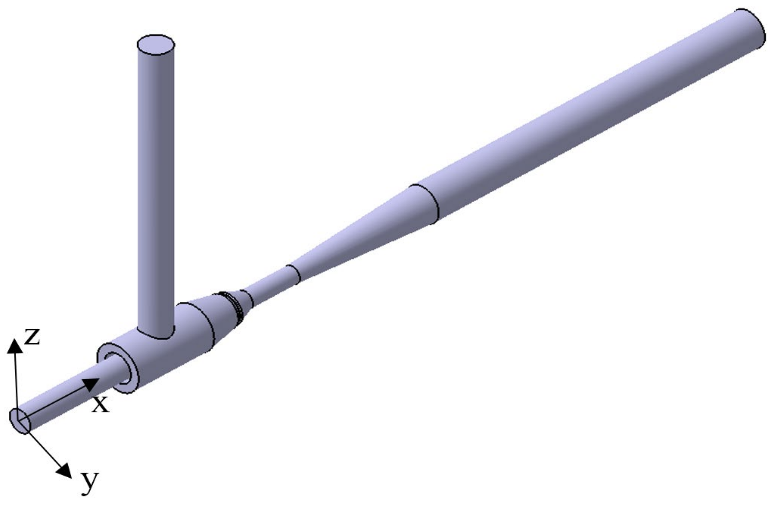
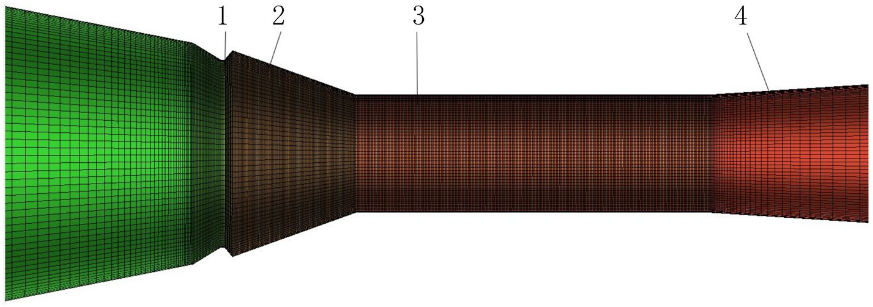
2.1. Jet Fish Pump

A jet fish pump comprises a primary duct, a suction duct, an annular nozzle, a suction chamber, a throat and a diffuser, as shown in Figure 1. The operating principle can be simplified as follows: the high-velocity primary flow entrains the secondary flow at the annular nozzle. Then, these flows exchange momentum and mix together in the suction chamber and throat, and then pass through the diffuser [23].
A jet fish pump with an area ratio m of 1.75 (m = At/Aj) was chosen as the initial calculation model [24,25]. The main structural parameters are shown in Table 1.
In addition, several non-dimensional parameters are calculated as follows:
q = Q s Q j
h = P c P s P j P c
η = q · h
where q is flow ratio, h is pressure ratio, η is jet fish pump efficiency; Qs and Qj are volumetric flow rates of the secondary and primary flows; Pc, Ps and Pj are total pressure of mixed, secondary and primary flows, respectively.

2.2. Description of the Optimization Problem

In our previous research, the numerical simulation feasibility of the three-dimensional turbulent flow field was tested in jet fish pumps, and the numerical calculation settings used in this paper are consistent with the cited papers [17]. Area ratio m, suction chamber inclination angle α and the length-to-diameter ratio of throat L/Dt are key structural parameters for damage probability in jet fish pumps. Therefore, they were taken as optimization design variables. Then, two groups of objectives of multi-objective optimization were taken, the radial pressure gradient ∇pr and efficiency η, the exposure strain rate e and efficiency η, respectively. The ∇pr and e were reduced to minimize the risk of fish damage, respectively. The multi-objective optimization problem was described as follows:
  • Optimization variable: T = (α, m, L/Dt)
  • Optimization object: Maximize {−∇pr, η}, Maximize {−e, η}.

2.3. Experimental Design

2.3.1. Uniform Experimental Design

According to uniform experimental design tables and usage tables of U30*(3013), three factors were applied to the jet fish pump, and the experimental design with a level number of 30 was selected for each element [26]. As mentioned in Section 2.2, prior to this, simulation calculations have been considered, α, m, and L/Dt were selected as the input parameters for the following multi-objective optimization. The variable value range of the structural parameters of the jet fish pump was set as follows:
  • Suction chamber inclination angle α: from 19° to 42.2°;
  • Area ratio m: from 1 to 4.625;
  • Throat length-diameter ratio L/Dt: from 2 to 4.03.

2.3.2. Sample Space Solution

The value ranges of α, m, and L/Dt were equally divided into 30 groups, and the structures of different combinations in these 30 groups were subjected to inverse problem design calculations. According to the above uniform test table, the test arrangement was carried out. 30 groups of jet fish pumps with different structural parameters were used to perform the three-dimensional modeling of the fluid domain as shown in Figure 2. A total of 30 groups of jet fish pumps with different structural parameters were meshed and the parts with complicated hydraulic factors were meshed densely in Figure 3. After grid independence verification, the total number of design grids of 30 groups of jet fish pump models with different structural parameters was about 5.5 million. Working conditions were consistent during the calculation of each group of models. According to the experiment results, primary and secondary flow rates were set as 80.08 m3/h and 40.89 m3/h, respectively. The outlet pressure was set as 18,270 Pa. A realizable k-ε model was used, SIMPLEC pressure-velocity coupling algorithm was adopted and the second-order upwind style discretization was adopted. Standard wall parameters were selected for each wall. Based on numerical simulation, the exposure strain rate e, radial pressure gradient ∇pr and overall efficiency η of 30 groups of jet fish pumps with different structures were obtained. Among them, the values of ∇pr and e were taken at the near wall of the throat y/Rt = 0.9 and y/Rt = 0.75, respectively.
The sample space was solved according to the simulation calculation method and all the sample space information obtained is shown in Table 2. There was a complicated non-linear relationship between ∇pr, η, e and α as well as m and L/Dt. Moreover, ∇pr and η as well as e and η were also coupled with each other.

2.4. Neural Network Design

The relationship between α, m, L/Dt and η as well as ∇pr, and e were complex nonlinear relationships and there was no empirical formula to refer to. Therefore, the BP neural network can better approximate the models of input structure parameters η, ∇pr, and e. After the mapping relationship was fitted, it was optimized with the NSGA-II multi-objective genetic algorithm.

2.4.1. Normalization of Sample Data

In the sample data, due to the difference of several orders of magnitude between η, ∇pr and e, the neural network will have slow convergence and a long training time during neural network training. Data input with an extensive data range may play a more prominent role in pattern classification, and vice versa, and even data annihilation may occur. In addition, the value range of the activation function of the neural network output layer is limited, so the trained objective function should also be mapped to the value range of the activation function. To avoid this error caused by the characteristics of the data, before BP neural network modeling, the data needed to be normalized first. The data were normalized to the range of [0, 1] according to Equation (4), as shown in Table 3.
Y = X   X min X max X min
In the formula, Y is the normalized value of the initial sample data; X is the value of the initial data; Xmax is the maximum value in the initial data set; Xmin is the minimum value in the initial data set.

2.4.2. Determination of the Number of Hidden Nodes

The number of hidden nodes of the BP neural network had a greater impact on the final training prediction effect [27]. When the number of hidden nodes is small, the learning effect of the neural network is poor, the training times need to be increased, and the training accuracy is low. When the number of hidden nodes is large, the training time is long, and the neural network is prone to overfitting. Therefore, this paper randomly divided 30 groups of training samples into a training set (25) and a test set (5). The loop algorithm was used to test the error of the neural network when the number of hidden nodes is 1–15. The error between the predicted and actual results was used to determine the number of hidden nodes. Among them, the hidden layer activation function selected tansig, the output layer activation function selected purelin, and the training function selected traingx [28]. After a total of 15 cycles, the original samples of the test set and the sum squared errors of the prediction of 15 groups of different hidden nodes were obtained, as shown in Figure 4. When the number of hidden nodes was 12, the error of the prediction efficiency was the smallest, so the hidden nodes of the BP neural network for the prediction efficiency were set to 12. Similarly, the number of hidden nodes of the BP neural network for predicting the pressure gradient and the exposure strain rate was set to 10 and 14.

2.4.3. Comparison of BP Neural Network Construction

The BP neural network was used to model and analyze the sample data. Then, the fitted mapping function was used as the fitness function of the NSGA-II multi-objective genetic algorithm for multi-objective optimization. The BP neural network used three structural parameters α, m, and L/Dt as input. η, ∇pr and e were output, and the hidden layers were 12, 10, and 14 neurons, respectively. The hidden layer activation function selected the tangent sigmoid function tansig, the output layer selected the linear transfer function purelin, and the training function selected the weight function tradingdm function. A three-layer BP neural network was established through the newff function, which was called by the following format:
net = newff ( pn , tn , 12 , { tansig , purelin } , traingdm )
where pn is the normalized training sample data matrix, and tn is the normalized target sample data matrix. MATLAB was used to model and train the BP neural network. There were 30 sets of samples in the above sample space, of which 25 groups in the sample space were randomly selected for training the neural network, and the remaining 5 groups were used as the test set of the neural network. Five test sets were used to test the effect of neural network training. The BP neural network for η prediction was trained 50,000 times, the learning step was set to 0.05 and the mean square error of the result was set to 10−5. After the neural network was trained 38,206 times, the mean square error met the target value, and the performance of the BP neural network was stable. The neural network regression value was about 0.998, close to 1, indicating that the fitting was reasonable. With the same settings to predict ∇pr and e, the neural network trained 48,259 times and 34,460 times, respectively, when the mean square error reached 10−5, which met the training requirements.
Then, the prediction model was compared with the numerical simulation value. The result showed that the designed BP neural network had a high training accuracy and met the prediction accuracy of the nonlinear relationship function. According to the three BP neural network models established, MATLAB was used to program the three prediction models in the form of functions. The following NSGA-II multi-objective genetic algorithm will sort the fitness values according to this fitness function.

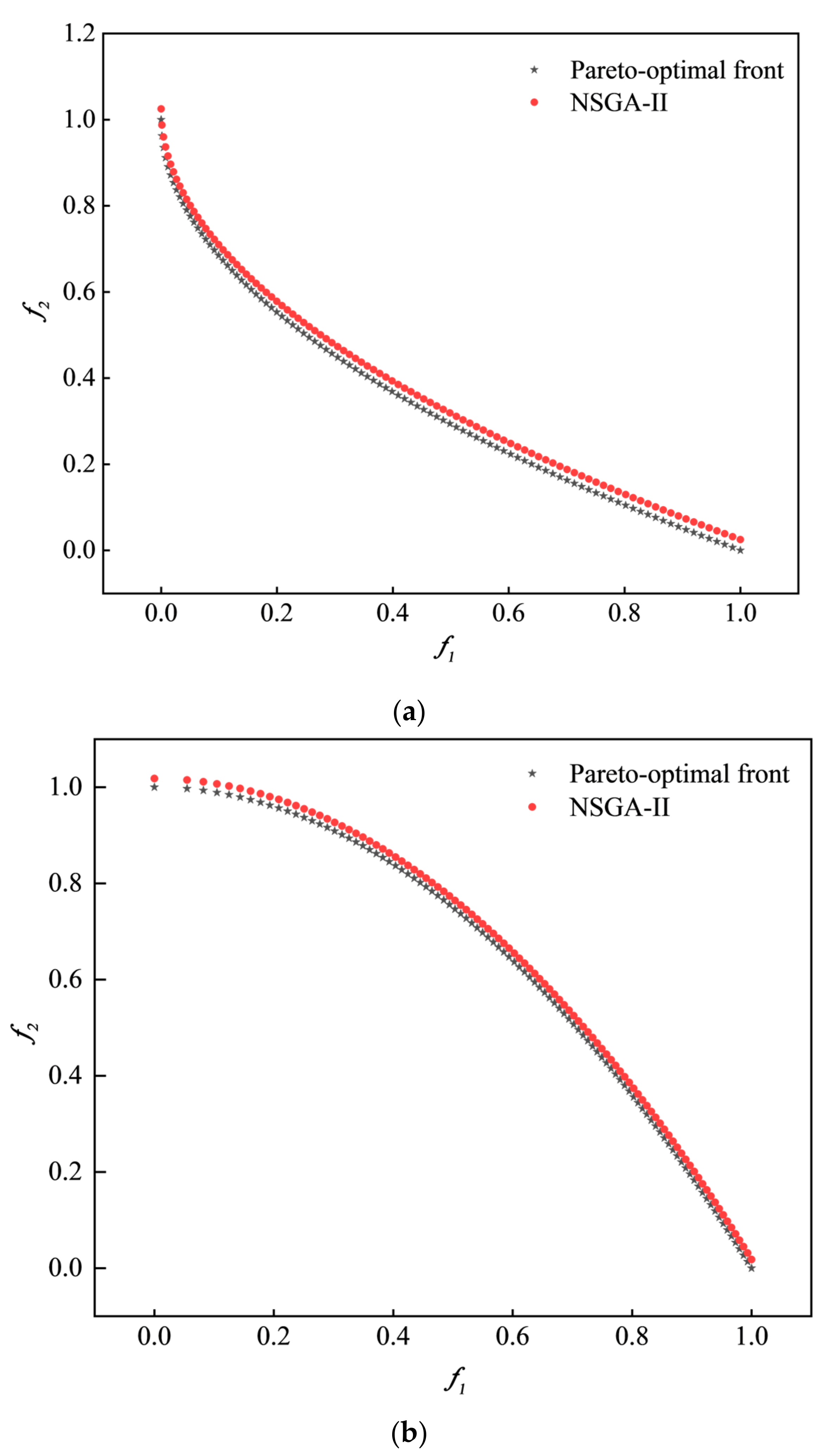
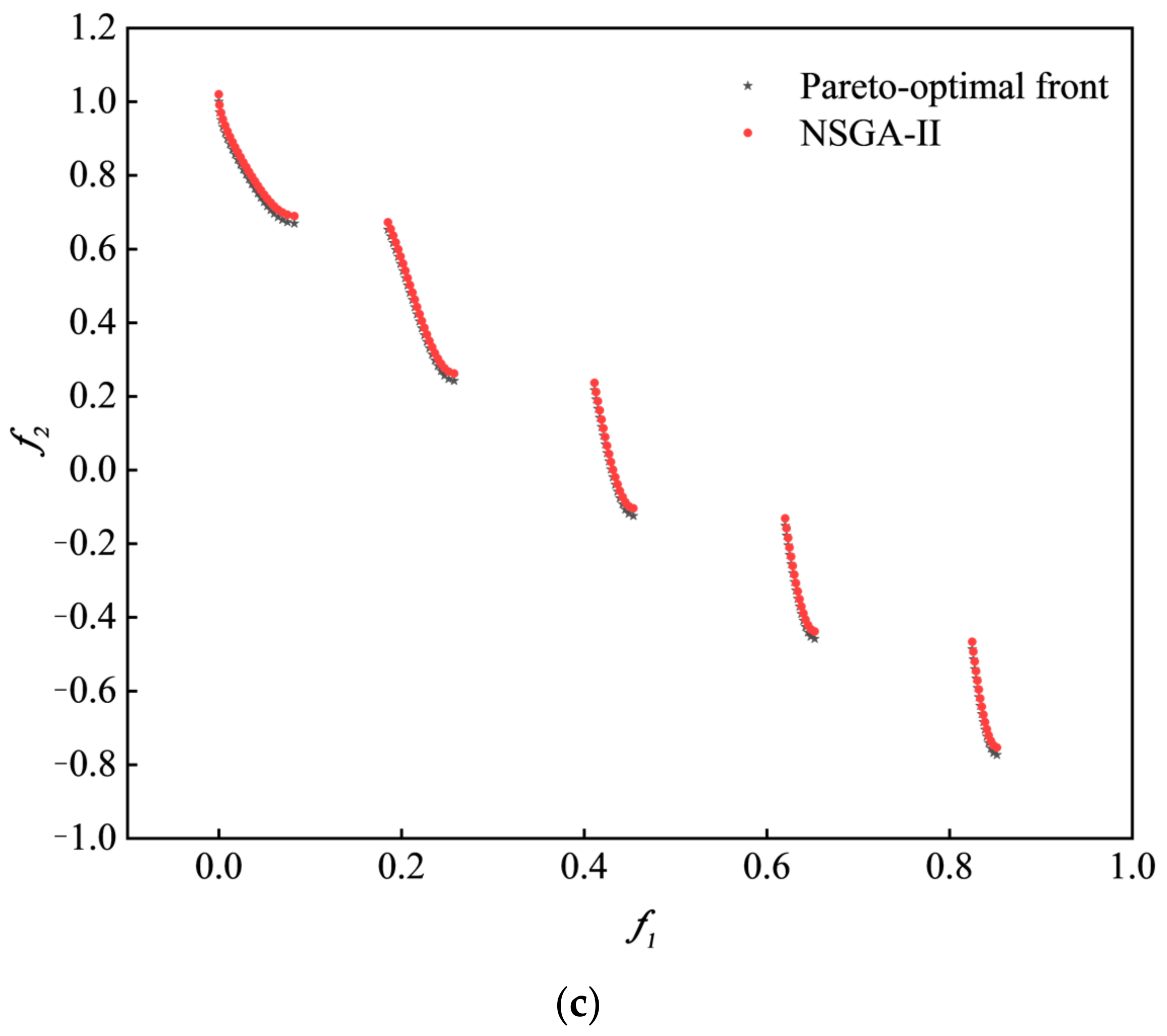
2.5. NSGA-II Genetic Algorithm Verification

Before using the NSGA-II multi-objective genetic algorithm for optimization, it was necessary to pass several test functions to verify the required reliability of the programmed genetic algorithm. The selected test function was introduced in Equations (6)–(8) [29].
ZDT1 function:
f 1 ( x ) = x 2 f 2 ( x ) = g ( x ) [ 1 f 1 ( x ) / g ( x ) ] , x i [ 0 , 1 ] , n = 30 g ( x ) = 1 + 9 ( i = 2 n x i ) n 1 , x = ( x 1 , x 2 , , x n ) T [ 0 , 1 ] n
ZDT2 function:
f 1 ( x ) = x 1 f 2 ( x ) = g ( x ) [ 1 ( x 1 g ( x ) ) 2 ] , x i [ 0 , 1 ] , n = 30 g ( x ) = 1 + 9 ( i = 2 n x i ) n 1 , x = ( x 1 , x 2 , , x n ) T [ 0 , 1 ] n
ZDT3 function:
f 1 ( x ) = x 1 f 2 ( x ) = g ( x ) [ 1 f 1 ( x ) g ( x ) ( 1 sin ( 10 π x 1 ) ) ] , x i [ 0 , 1 ] , n = 30 g ( x ) = 1 + 9 ( i = 2 n x i ) n 1 , x = ( x 1 , x 2 , , x n ) T [ 0 , 1 ] n
Programming calculations were performed separately through the NSGA-II algorithm for the above three test functions. The main program remains unchanged; only the fitness function in the sub-function was changed, and the result obtained was compared with the ideal Pareto frontier of the corresponding function. The result is shown in Figure 5 below. According to the comparison chart of the three reliability function verification results of ZDT1, ZTD2 and ZDT3 in the figure below, the Pareto solution set produced by the NSGA-II multi-objective genetic algorithm written in this paper was consistent with the ideal Pareto solution set and was more consistent in value. Therefore, it was reliable that this paper used the NSGA-II multi-objective genetic algorithm to optimize η and ∇pr as well as η, and e of the internal structural parameters of the jet fish pump.

3. Results and Discussion

3.1. Basic Analysis of Optimization Results

After verifying the reliability of the above experimental design arrangement, the neural network mapping function was established, as well as the NSGA-II multi-objective genetic optimization function. Therefore, the structural parameters of the jet fish pump can be optimized. The optimization operation of NSGA-II was the optimization of ∇pr-η and e-η. In this paper, the BP neural network was applied to approximate the non-linear function relationship between the structural parameters and the target. Then the NSGA-II multi-objective genetic algorithm was used to cooperate with each other to optimize. Among them, the initial population of the NSGA-II multi-objective genetic algorithm was set to 200. The number of iterations was set to 500. The tournament selection method was used for selection, the genetic crossover probability was set to 0.9, and the mutation probability was set to 0.3. After 500 iterations of the NSGA-II multi-objective genetic algorithm, the corresponding non-dominated solution set can be obtained.
Figure 6 and Figure 7 showed ∇pr-η Pareto solution set and e-η Pareto solution set obtained after optimization by the NSGA-II multi-objective genetic algorithm. According to the figure, the obtained ∇pr-η Pareto frontier and e-η Pareto front curves were smooth, with good distribution. It can better reflect the excellent ability of the NSGA-II multi-objective genetic algorithm to search for Pareto non-dominated solutions [30].
According to Table 4, when m was approximate to 2.1, α was about 20°, and L/Dt was about 2.2, the jet fish pump could achieve greater efficiency. At the same time, we have noticed that ∇pr at the inlet section of the jet fish pump throat was relatively small. According to Table 5, when m was about 1.5, α and L/Dt were approximately 19.15° and 2.5, respectively, η was slightly improved, and the fish was less likely to be damaged by the shear flow in the fish pump. Due to a large number of solutions, this research followed the principle of high to low fitness; the information of each of the 5 Pareto solutions was selected, as shown in Table 5 and Table 6 below.

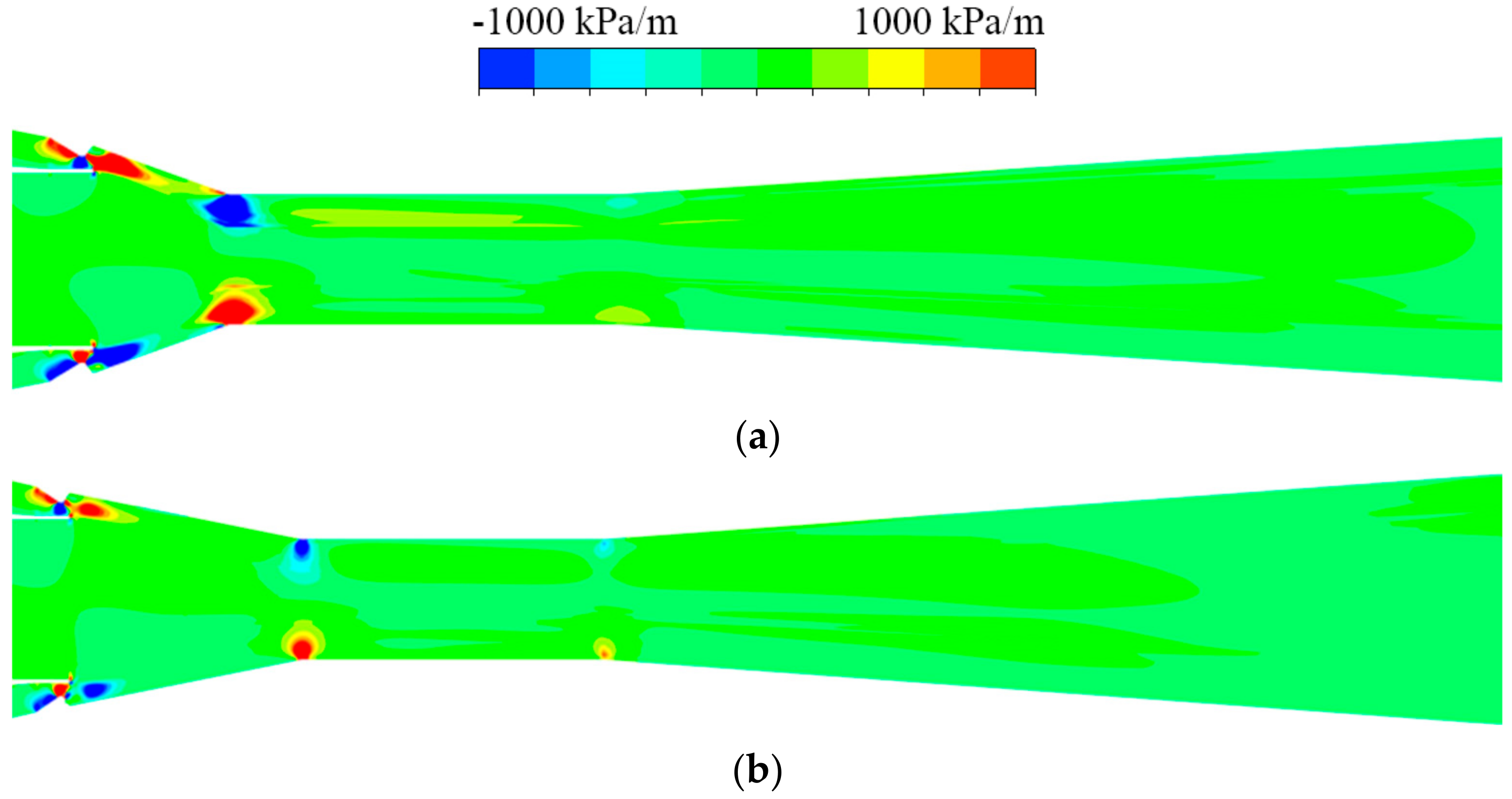
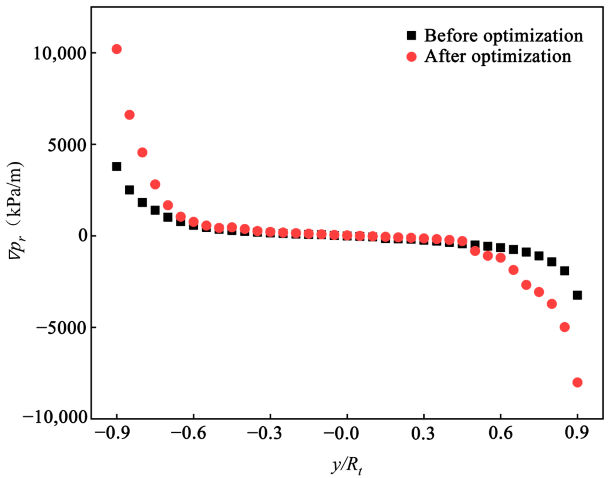
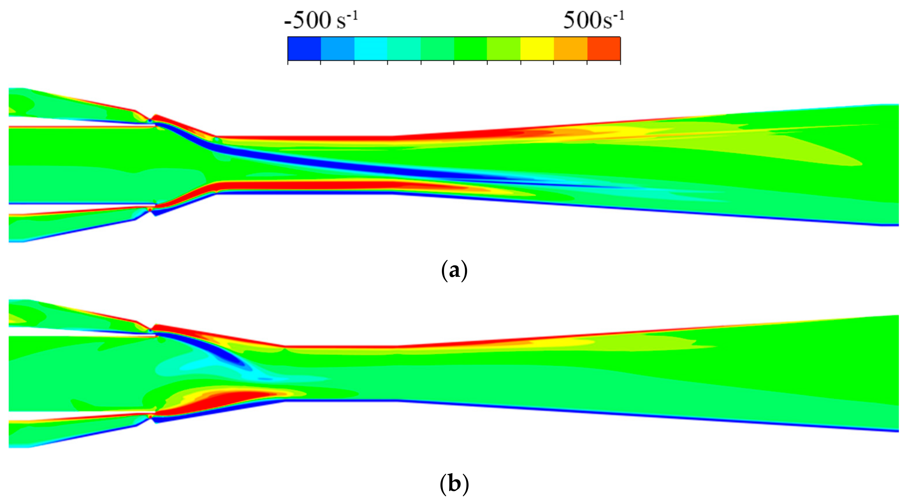
3.2. Analysis of Internal Flow Field before and after Optimization

The internal flow field with a high fitness value was numerically simulated. The simulation calculation settings were consistent with the flow field settings in Section 2.3.2. Then the simulation calculation results were compared with the predicted results and individual target values before NSGA-II multi-objective genetic optimization. The comparison results are shown in Table 6. According to the table, it can be seen that ∇pr and η inside the optimized jet fish pump were smaller than that in the initial structure. After multi-objective optimization, ∇pr at the throat inlet section y/Rt = 0.9 and e at the throat inlet section y/Rt = 0.75 were about 2/5 and 1/8 of the values in the initial jet fish pump, respectively. In addition, η was increased by 4.8%.
Figure 8 shows diagrams of ∇pr inside the jet fish pump before and after optimization by the NSGA-II multi-objective genetic algorithm. In this figure, the distribution areas where ∇pr was higher than 1000 kPa/m after optimization were similar to those before optimization. They were all distributed from the outlet of the annular nozzle to the front part of the suction chamber, at the end of the suction chamber and at the throat inlet section. Near the front wall surface of the shrinking chamber, the volume of ∇pr higher than 1000 kPa/m after optimization was about 1/3 of that before optimization. Before optimization, the region with high ∇pr accounted for about half of the inlet of the throat. After multi-objective genetic optimization, even though the high-pressure gradient region still appeared at the end of the suction chamber and the entrance of the throat, the range of this region was reduced. Therefore, the probability of fish being damaged by the pressure gradient was smaller than that before optimization.
As shown in Figure 9, ∇pr before and after optimization was further compared and analyzed. After NSGA-II multi-objective optimization, ∇pr distribution law of the jet fish pump at the inlet section of its throat was the same as before optimization. ∇pr near the centerline of the jet fish pump was small or even close to zero. As the radial position gradually approached the wall surface, ∇pr gradually increased and the magnitude of the increase was also more significant. Numerically, the difference in ∇pr near the centerline of the inlet section of the jet fish pump throat before and after optimization was relatively small. ∇pr, where the optimized radial position y/Rt was between 0.75 and 0.9 and between −0.9 and −0.75, was significantly different from ∇pr before optimization; ∇pr in this interval before optimization was about 2~2.5 times that after optimization. In addition, the corresponding force on fish gills and scales after optimization was only about 2/5 of that before optimization. Therefore, the risk of damage to fish due to ∇pr was also reduced.
The cloud diagram of the internal flow field of the jet fish pump optimized by the NSGA-II with e higher than 500 s−1 is shown in Figure 10. Similar to the distribution trend before optimization, e near the axis of the jet fish pump optimized by the multi-objective structure was relatively small. After optimization, there were still dangerous areas inside the jet fish pump due to shear flow. The scope of the dangerous area was significantly reduced compared to before optimization, and it was mainly distributed in the interior of the suction chamber and the area near the wall of the diffuser inlet. The dangerous area at the diffuser inlet of the optimized jet fish pump was slightly smaller than that of the initial model. Before the optimization, the dangerous area inside the throat was more extensive and existed in the entire throat. However, the dangerous area inside the optimized throat only existed at the entrance of the throat, and as the flow progressed, e gradually decreased. In addition, the area where e was higher than 500 s−1 was analyzed and calculated separately. Before optimization, the dangerous area was 4.5 × 10⁻⁴ m3, and the dangerous area after NSGA-II optimization was reduced to 2.5 × 10⁻⁴ m3. The scope of the dangerous area was reduced by nearly 1/2. Therefore, the probability of damage to the transported fish due to shear flow was relatively small.

4. Conclusions and Future Direction

Based on the numerical simulation method, this study calculated the flow characteristics of jet fish pumps with different structural parameters. According to numerical results and the fish injury threshold of typical hydraulic factors, the internal mapping between key structural parameters, including suction chamber inclination angle, area and throat length-diameter ratios, and fish injuries was established using a BP neural network. Then, this mapping relationship was solved by an NSGA-II multi-objective genetic algorithm. The main conclusions are summarized as follows:
(1)
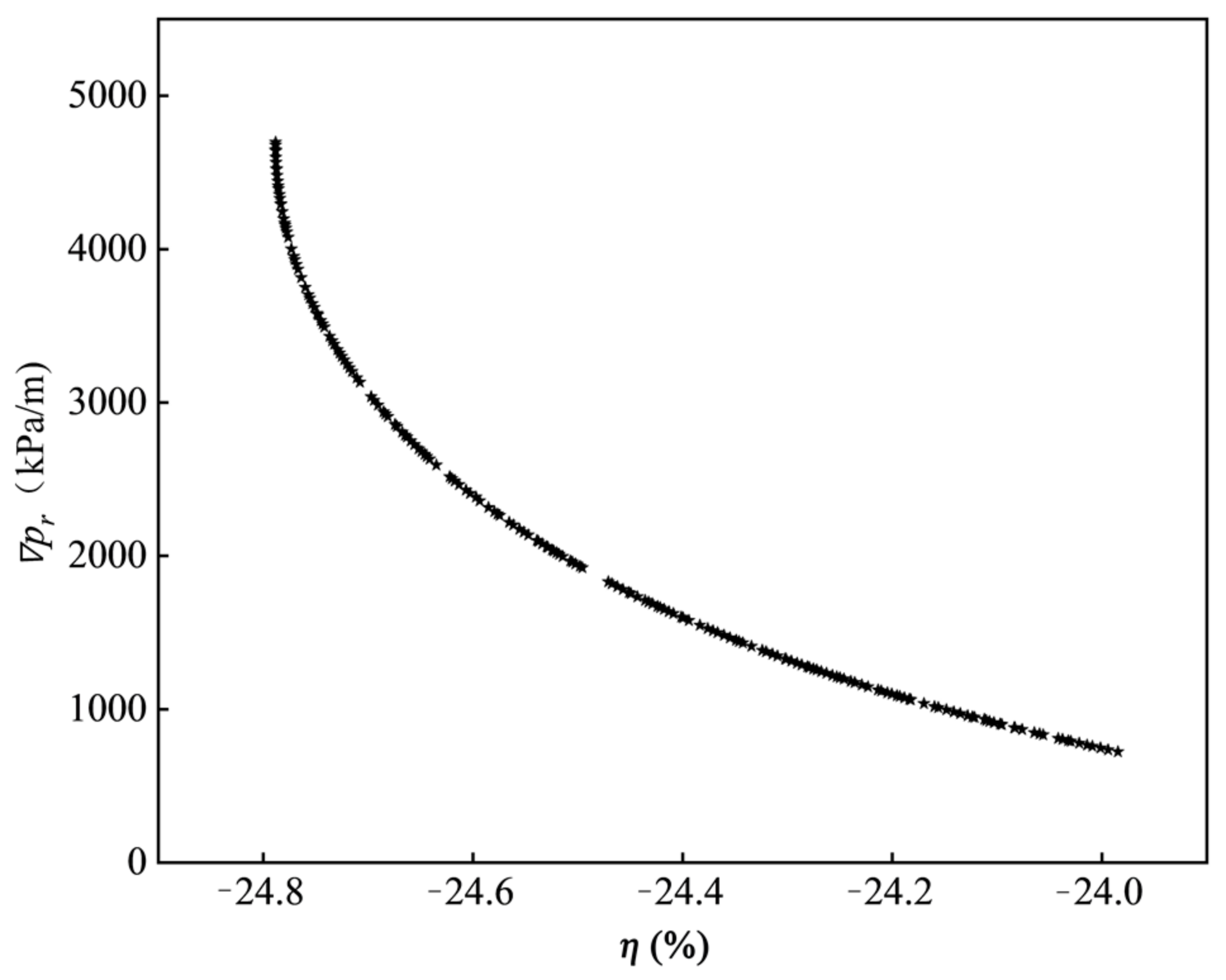
By comparing with Pareto solution sets, the reality of the NSGA-II multi-objective genetic algorithm is verified. This multi-objective genetic algorithm can optimize η and ∇pr as well as η and e of the internal structural parameters of the jet fish pump. The obtained ∇pr-η Pareto frontier and e-η Pareto front can reflect the excellent ability of the NSGA-II multi-objective genetic algorithm to search for Pareto non-dominated solutions.
(2)
According to optimization results, efficiency, radial pressure gradient and exposure strain rate cannot be optimal at the same time. The optimized structural parameters considering ∇pr-η are different from those considering e-η.
(3)
Aiming at high jet pump efficiency and low radial pressure gradient, the optimized structure combination is that m = 2.1, α = 20°and L/Dt = 2.2. The radial pressure gradient in the jet fish pump with this structure combination can be decreased to about 40% of that in the origin jet fish pump before optimization.
(4)
Aiming at high jet pump efficiency and low exposure strain rate, the optimized structure combination is that m = 1.5, α = 19.15° and L/Dt = 2.5. The exposure strain rate and dangerous area scope in the jet fish pump with this structure combination can be decreased at about 12.5% and 50% of that in the origin jet fish pump before optimization, respectively. In addition, the efficiency of this jet fish pump with optimized structure is increased by 4.8%.
Notwithstanding our present results on the jet fish pumps, there is still a lot of work needed in the future. Key issues include the following:
(1)
The motion of fish could affect the distribution of the flow field, which was ignored in this research. For further study, researchers could pay more attention to the swimming of fish and achieve a more optimized model of a jet fish pump.
(2)
Limited by computing resources, input samples of structural parameters are relatively few. For additional research, it is necessary to expand the range of structural parameters and increase the level of input variables to obtain a more accurate internal mapping relationship.
(3)
In the present research, two objectives of ∇pr-η and e-η were optimized by the NSGA-II genetic algorithm, respectively. For the following research, multi-objective optimization combining η with ∇pr and e could be carried out and provide a theoretical basis for high-efficiency and low fish-loss jet fish pump design.

Author Contributions

Conceptualization, M.X.; methodology, G.Z., D.W. and J.M.; validation, J.Z.; investigation, M.X.; writing—original draft preparation, M.X. and B.H.; writing—review and editing, M.X. and G.Z.; visualization, S.Z.; supervision, D.W.; project administration, Y.R.; funding acquisition, J.M. All authors have read and agreed to the published version of the manuscript.

Funding

This research was funded by National Natural Science Foundation of China (Project No. 51909235), Zhejiang Province Public Welfare Technology Application Research Project (Project Nos. LGG22E090001 and LGG21E090003) and Zhejiang Post-Doctoral Preferential Fund Project (Project No. ZJ2021115).

Data Availability Statement

Not applicable.

Conflicts of Interest

The authors declare no conflict of interest.

References

  1. FAO. The State of World Fisheries and Aquaculture 2020; FAO: Rome, Italy, 2020. [Google Scholar]
  2. Long, X.; Xu, M.; Qiao, L.; Zou, J. Impact of the internal flow in a jet fish pump on the fish. Ocean Eng. 2016, 126, 313–320. [Google Scholar] [CrossRef]
  3. Xiao, L.; Long, X.; Li, L.; Xu, M.; Wu, N.; Wang, Q. Movement characteristics of fish in a jet fish pump. Ocean Eng. 2015, 108, 480–492. [Google Scholar] [CrossRef]
  4. Long, X.; Xu, M.; Wang, J.; Zou, J.; Ji, B. An experimental study of cavitation damage on tissue of Carassius auratus in a jet fish pump. Ocean Eng. 2019, 174, 43–50. [Google Scholar] [CrossRef]
  5. Moses, D.; Colt, J. Impact of fish feed on airlift pumps in aquaculture systems. Aquacult. Eng. 2018, 80, 22–27. [Google Scholar] [CrossRef]
  6. Xu, M.; Ji, B.; Zou, J.; Long, X. Experimental investigation on the transport of different fish species in a jet fish pump. Aquacult Eng. 2017, 79, 42–48. [Google Scholar] [CrossRef]
  7. Huang, X.; Guo, G.; Tao, Q. Research on key technology and design for jet fish pump. SCFS 2007, 3, 41–46. (In Chinese) [Google Scholar]
  8. Wu, N.; Li, L.; Hou, J.; Long, X.; Xu, M.; Su, Y.; Lin, W. Stress reponse of grass carp after passing the jet fish pump. J. Huazhong Agricult. Univ. 2016, 35, 75–83. (In Chinese) [Google Scholar]
  9. Xu, M.; Long, X.; Mou, J.; Ji, B.; Ren, Y. Impact of fish locomotion on the internal flow in a jet fish pump. Ocean Eng. 2019, 187, 106227. [Google Scholar] [CrossRef]
  10. Neitzel, D.A.; Richmond, M.C.; Dauble, D.D.; Mueller, R.P.; Moursund, R.A.; Abernethy, C.S.; Guensch, G.R. Laboratory Studies on the Effects of Shear on Fish; Pacific Northwest National Laboratory: Richland, WA, USA, 2000.
  11. Neitzel, D.A.; Dauble, D.D.; Čada, G.F.; Richmond, M.C.; Guensch, G.R.; Mueller, R.P.; Amidan, B. Survival estimates for juvenile fish subjected to a laboratory-generated shear environment. Trans. Am. Fish. Soc. 2004, 133, 447–454. [Google Scholar] [CrossRef]
  12. Guensch, G.R.; Mueller, R.P.; McKinstry, C.A.; Dauble, D.D. Evaluation of Fish-Injury Mechanisms during Exposure to a High-Velocity Jet; Pacific Northwest National Laboratory: Richland, WA, USA, 2003.
  13. Pribyl, A.L.; Kent, M.L.; Parker, S.J.; Schreck, C.B. The response to forced decompression in six species of pacific rockfish. Trans. Am. Fish. Soc. 2011, 140, 374–383. [Google Scholar] [CrossRef]
  14. Hannah, R.W.; Parker, S.J.; Matteson, K.M. Escaping the surface: The effect of capture depth on submergence success of surface-released Pacific rockfish. N. Am. J. Fish Manag. 2008, 28, 694–700. [Google Scholar] [CrossRef]
  15. Hannah, R.W.; Rankin, P.S.; Penny, A.N.; Parker, S.J. Physical model of the development of external signs of barotrauma in Pacific rockfish. Aquat. Biol. 2008, 3, 291–296. [Google Scholar] [CrossRef]
  16. Xu, M.; Long, X.; Mou, J.; Wu, D.; Zhou, P.; Gu, Y. Impact of pressure gradients on fish scales in a jet fish pump. Biosyst. Eng. 2020, 191, 27–34. [Google Scholar] [CrossRef]
  17. Xu, M.; Mou, J.; Wu, D.; Zhou, P.; Gu, Y.; Zheng, S. Probability evaluation of hydrodynamic shear damage for fish passing through jet fish pumps. Int. J. Fluid Mach. Syst. 2020, 13, 536–542. [Google Scholar] [CrossRef]
  18. Wong, B.K.; Lai, V.S.; Lam, J. A bibliography of neural network business applications research: 1994–1998. Comput. Oper. Res. 2000, 27, 1045–1076. [Google Scholar] [CrossRef]
  19. He, C.; Gu, Y.; Zhang, J.; Ma, L.; Yan, M.; Mou, J.; Ren, Y. Preparation and modification technology analysis of ionic Polymer-Metal Composites (IPMCs). Int. J. Mol. Sci. 2022, 23, 3522. [Google Scholar] [CrossRef]
  20. Zhou, Y.; Cao, S.; Kosonen, R.; Hamdy, M. Multi-objective optimisation of an interactive buildings-vehicles energy sharing network with high energy flexibility using the Pareto archive NSGA-II algorithm. Energy Convers. Manag. 2020, 218, 113017. [Google Scholar] [CrossRef]
  21. Luo, H.; Zhou, P.; Shu, L.; Mou, J.; Zheng, H.; Jiang, C.; Wang, Y. Energy performance curves prediction of centrifugal pumps based on constrained PSO-SVR model. Energies 2022, 15, 3309. [Google Scholar] [CrossRef]
  22. Yang, D.; Zhou, X.; Yang, Z.; Jiang, Q.; Feng, W. Multi-objective optimization model for flexible job shop scheduling problem considering transportation constraints: A comparative study. In Proceedings of the 2020 IEEE Congress on Evolutionary Computation (CEC), Glasgow, UK, 19 July 2020; pp. 1–8. [Google Scholar]
  23. Elger, D.F.; Taylor, S.J.; Liou, C.P. Recirculation in an annular-type jet pump. J. Fluid Eng. T ASME 1994, 116, 735–740. [Google Scholar] [CrossRef]
  24. Yang, X.; Long, X.; Kang, Y.; Xiao, L. Application of constant rate of velocity or pressure change method to improve annular jet pump performance. Int. J. Fluid Mach. Syst. 2013, 6, 137–143. [Google Scholar] [CrossRef] [Green Version]
  25. Xiao, L.; Long, X.; Lyu, Q.; Hu, Y.; Wang, Q. Numerical investigation on the cavitating flow in annular jet pump under different flow rate ratio. In IOP Conference Series: Earth and Environmental Science; IOP Publishing: Bristol, UK, 2014; p. 052001. [Google Scholar]
  26. Fang, K.; Liu, M.-Q.; Qin, H.; Zhou, Y. Theory and Application of Uniform Experimental Designs; Springer: Berlin/Heidelberg, Germany, 2018; p. 221. [Google Scholar]
  27. Qi, S.; Jin, K.; Li, B.; Qian, Y. The exploration of internet finance by using neural network. J. Comput. Appl. Math. 2020, 369, 112630. [Google Scholar] [CrossRef]
  28. Chang, L.; Xu, X.; Liu, Z.; Qian, B.; Xu, X.; Chen, Y. BRB prediction with customized attributes weights and tradeoff analysis for concurrent fault diagnosis. IEEE Syst. J. 2020, 15, 1179–1190. [Google Scholar] [CrossRef]
  29. Liu, J.; Chen, X. An improved NSGA-II algorithm based on crowding distance elimination strategy. Int. J. Comput. Int. Sys. 2019, 12, 513. [Google Scholar] [CrossRef] [Green Version]
  30. Gao, X.; Chen, B.; He, X.; Qiu, T.; Li, J.; Wang, C.; Zhang, L. Multi-objective optimization for the periodic operation of the naphtha pyrolysis process using a new parallel hybrid algorithm combining NSGA-II with SQP. Comput. Chem. Eng. 2008, 32, 2801–2811. [Google Scholar] [CrossRef]
Figure 1. Sketch of jet fish pump structure. 1-suction duct; 2-primary duct; 3-suction chamber; 4-annular nozzle; 5-throat; 6-diffuser.
Energies 15 04104 g001
Figure 2. Computational domain model of jet fish pump.
Energies 15 04104 g002
Figure 3. Schematic diagram of local grid refinement. 1-annular nozzle; 2-suction chambers; 3-throat; 4-diffuser.
Energies 15 04104 g003
Figure 4. Sum squared error of BP neural network (η) in different hidden layer nodes.
Energies 15 04104 g004
Figure 5. Test function comparison diagram. (a) ZDT1; (b) ZDT2; (c) ZDT3.
Energies 15 04104 g005aEnergies 15 04104 g005b
Figure 6. Pareto solution set (∇pr-η).
Energies 15 04104 g006
Figure 7. Pareto solution set (e-η).
Energies 15 04104 g007
Figure 8. Internal radial pressure gradient before and after optimization. (a) Before optimization; (b) After optimization.
Energies 15 04104 g008
Figure 9. Internal radial pressure gradient before and after optimization (at inlet section of throat).
Energies 15 04104 g009
Figure 10. Internal exposure strain rate before and after optimization. (a) Before optimization; (b) After optimization.
Energies 15 04104 g010
Table 1. Structural parameters of jet fish pump.
ParameterDs(mm)Dp(mm)Dt(mm)Dd(mm)α(°)β(°)
Size8010060125397
Table 2. Sample space of multi-objective optimization.
NO.α/(°)mL/Dtpr/(kPa/m)e/(s−1)η/(%)
1193.253.475340942.54516.99
219.81.752.8428,115914.34918.75
320.64.1252.215410987.52816.90
421.42.6253.755570998.60716.92
522.21.1253.1258901097.28018.41
6233.52.4991331358.62016.66
723.824.0351871002.74019.24
824.64.3753.412,9001815.04014.41
925.42.8752.7782851512.28019.35
1026.21.3752.146086965.49816.81
11273.753.6813,6621892.40015.59
1227.82.253.0556821301.14022.12
1328.64.6252.4218,4772289.66013.02
1429.43.1253.9611,2871707.77018.19
1530.21.6253.3357341076.14020.76
163143.8915,7651085.12034.57
1731.82.53.4788961663.19021.87
1832.613.614614432.4141.85
1933.43.3752.9816,5001950.46017.21
2034.21.8752.3565581521.68023.88
21354.252.0723,9442276.48013.52
2235.82.753.2613,0592063.72021.08
2336.61.252.12556951081.48218.30
2437.43.625220,6662201.54016.31
2538.22.1253.5419,3131875.48023.56
26394.52.9128,2792403.17013.13
2739.832.2817,7162069.19019.39
2840.61.53.8273791098.20017.40
2941.43.8753.1927,1382437.37015.14
3042.22.3752.5613,4372015.68023.61
Table 3. Sample space of multi-objective optimization after data normalization.
NO.α/(°)mL/Dtpr/(kPa/m)e/(s−1)η/(%)
10.00000.62070.72410.09650.09650.4627
20.03450.20690.41380.99350.99350.5165
30.06900.86210.10340.09930.09930.4600
40.10340.44830.86210.10560.10560.4606
50.13790.03450.55170.00000.00000.5061
60.17240.68970.24140.24590.24590.4526
70.20690.27591.00000.05110.05110.5315
80.24140.93100.68970.39430.39430.3839
90.27590.51720.37930.21250.21250.5348
100.31030.10340.06900.04710.04710.4572
110.34480.75860.82760.42430.42430.4199
120.37930.34480.51720.11000.11000.6195
130.41381.00000.20690.61390.61390.3414
140.44830.58620.96550.33070.33070.4994
150.48280.17240.65520.07260.07260.5779
160.51720.82760.93100.50710.50711.0000
170.55170.41380.72410.23660.23660.6119
180.58620.00000.79310.06790.06790.0000
190.62070.65520.48280.53610.53610.4694
200.65520.24140.17240.14450.14450.6733
210.68970.89660.03450.82930.82930.3567
220.72410.48280.62070.40050.40050.5877
230.75860.06900.06160.11050.11050.5028
240.79310.72410.00000.70010.70010.4419
250.82760.31030.75860.64690.64690.6635
260.86210.96550.44831.00001.00000.3447
270.89660.55170.13790.58400.58400.5361
280.93100.13790.89660.17680.17680.4752
290.96550.79310.58620.95510.95510.4062
301.00000.37930.27590.41540.41540.6650
Table 4. Specific information of optimized Pareto solution (∇pr-η).
NO.α/(°)mL/Dtpr(kPa/m)η/(%)Fitness
10.041350.2891100.0912703618.7624.750.0414
20.039820.2917320.0803833343.8824.720.0385
30.041190.3236660.0953243159.6724.700.0325
40.042110.3105890.0857143379.5824.730.0314
50.040260.3292140.0835423202.4124.710.0276
Table 5. Specific information of optimized Pareto solution (e-η).
NO.α/(°)mL/Dtpr(kPa/m)η/(%)Fitness
10.0066120.1474480.248935212.6726.150.0654
20.0059050.1483080.247737257.1426.280.0416
30.0069460.1642640.238342218.6326.180.0363
40.0070370.1530770.244936220.2026.190.0342
50.0068750.1677780.239856203.7926.100.0327
Table 6. Comparison of optimization results (∇pr-η and e-η).
Valuepr/(kPa/m)η/(%)e/(s−1)η/(%)
Initial value10,20023.831572.1923.83
Predictive value3618.7624.75212.6726.15
Analog value3787.7323.98205.9425.03
Publisher’s Note: MDPI stays neutral with regard to jurisdictional claims in published maps and institutional affiliations.

