
Improved Prediction of Aerodynamic Loss Propagation as Entropy Rise in Wind Turbines Using Multifidelity Analysis


Abstract
:
1. Introduction
2. Methodology
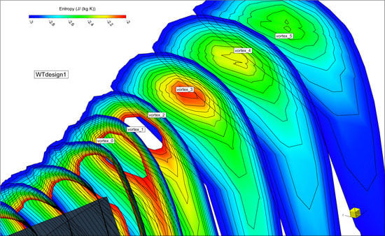
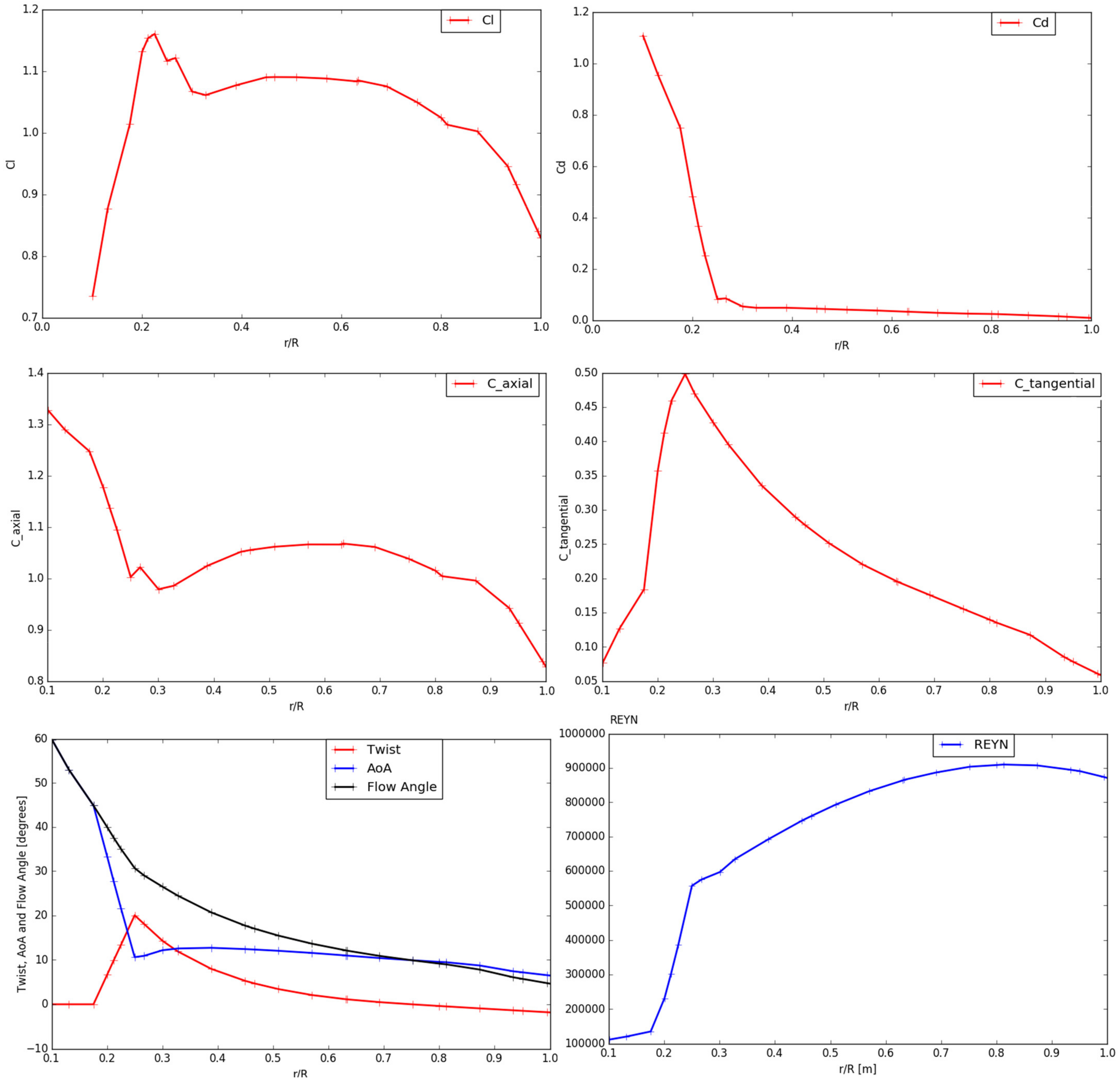
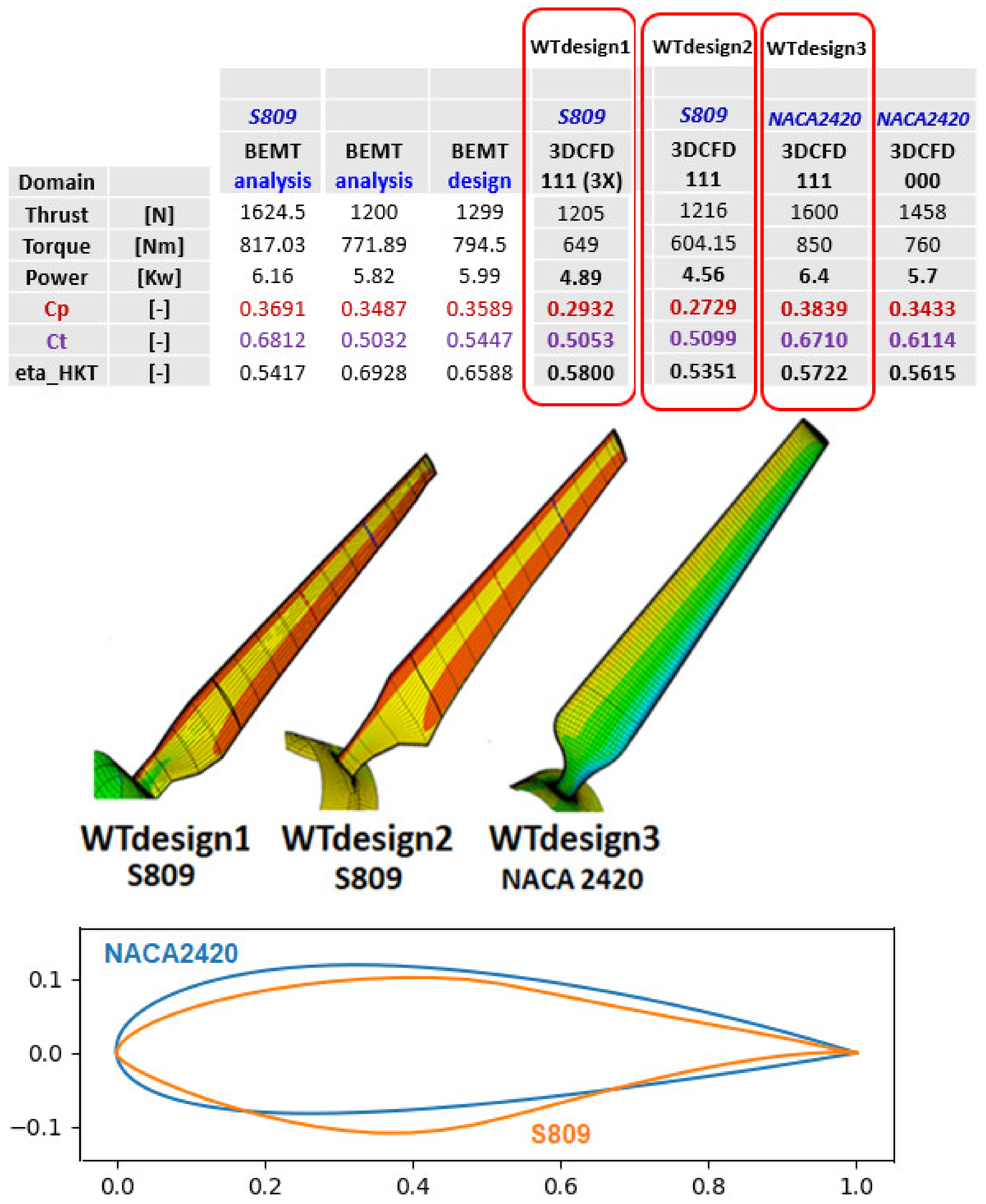
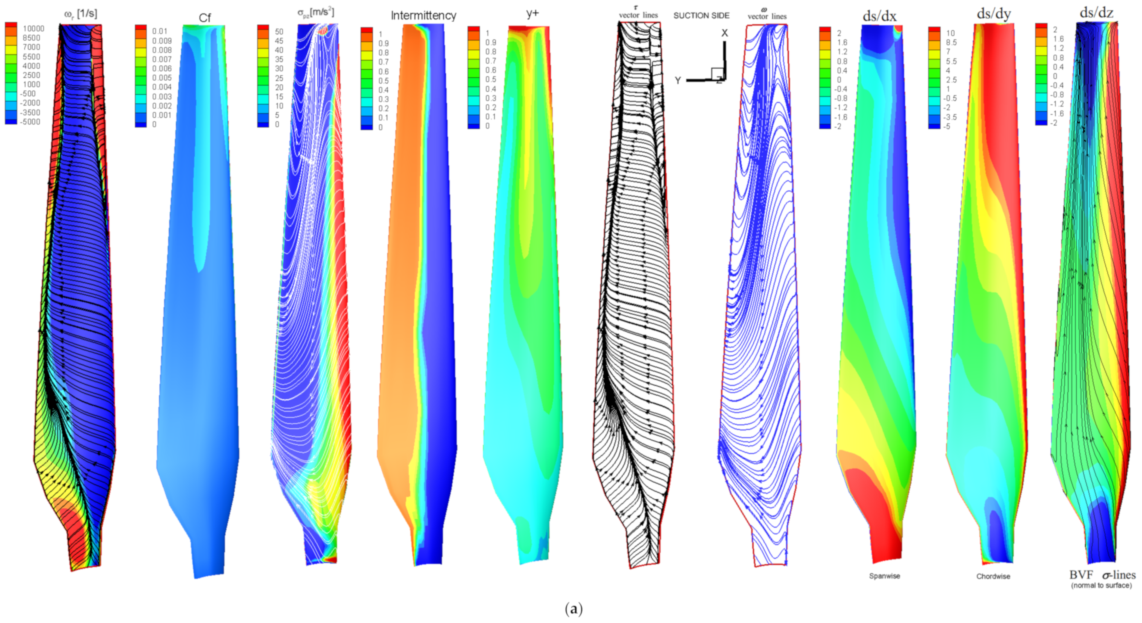
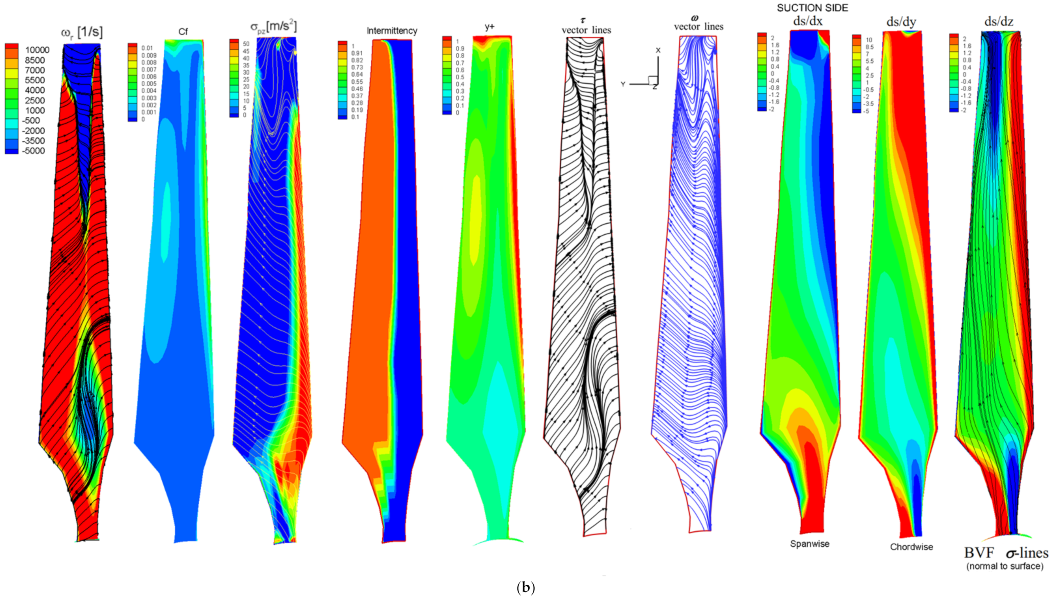
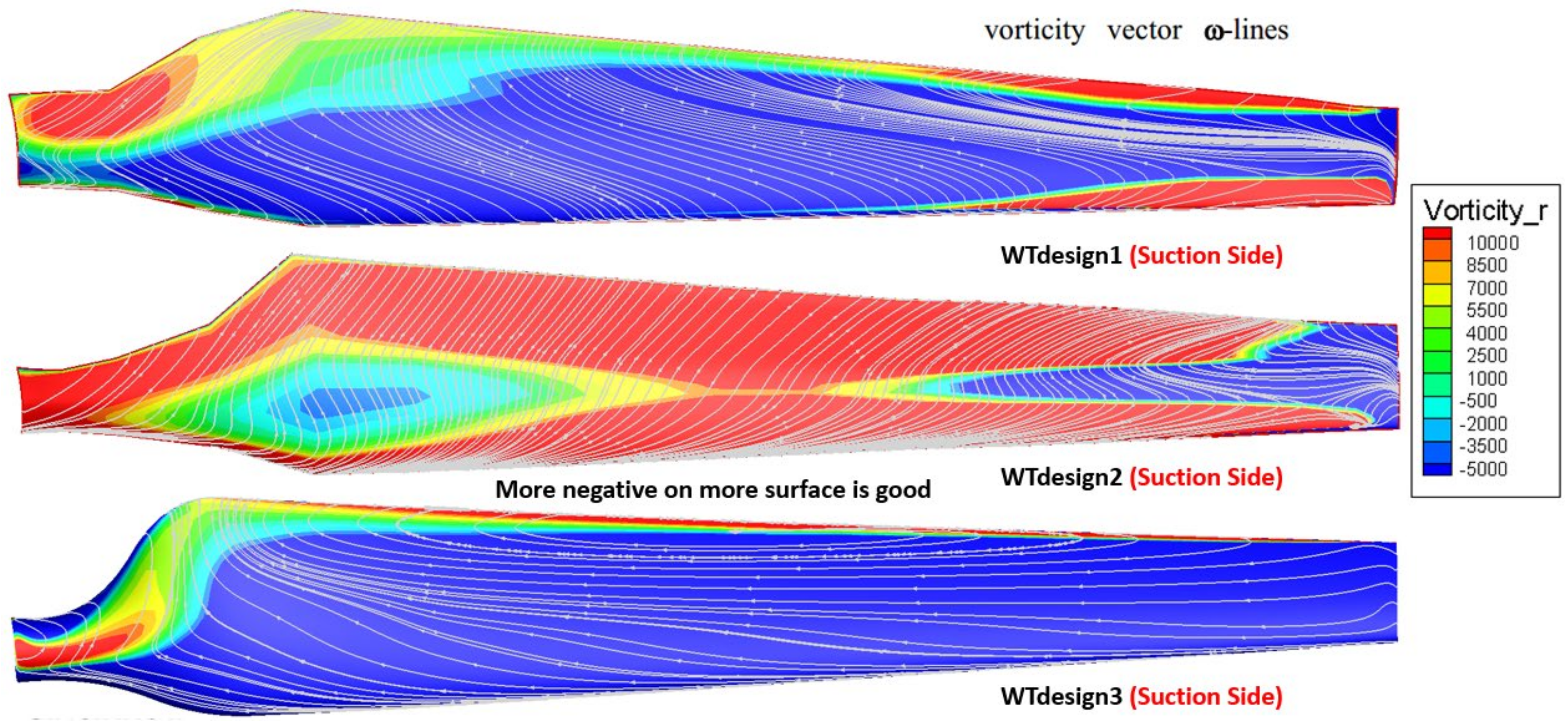
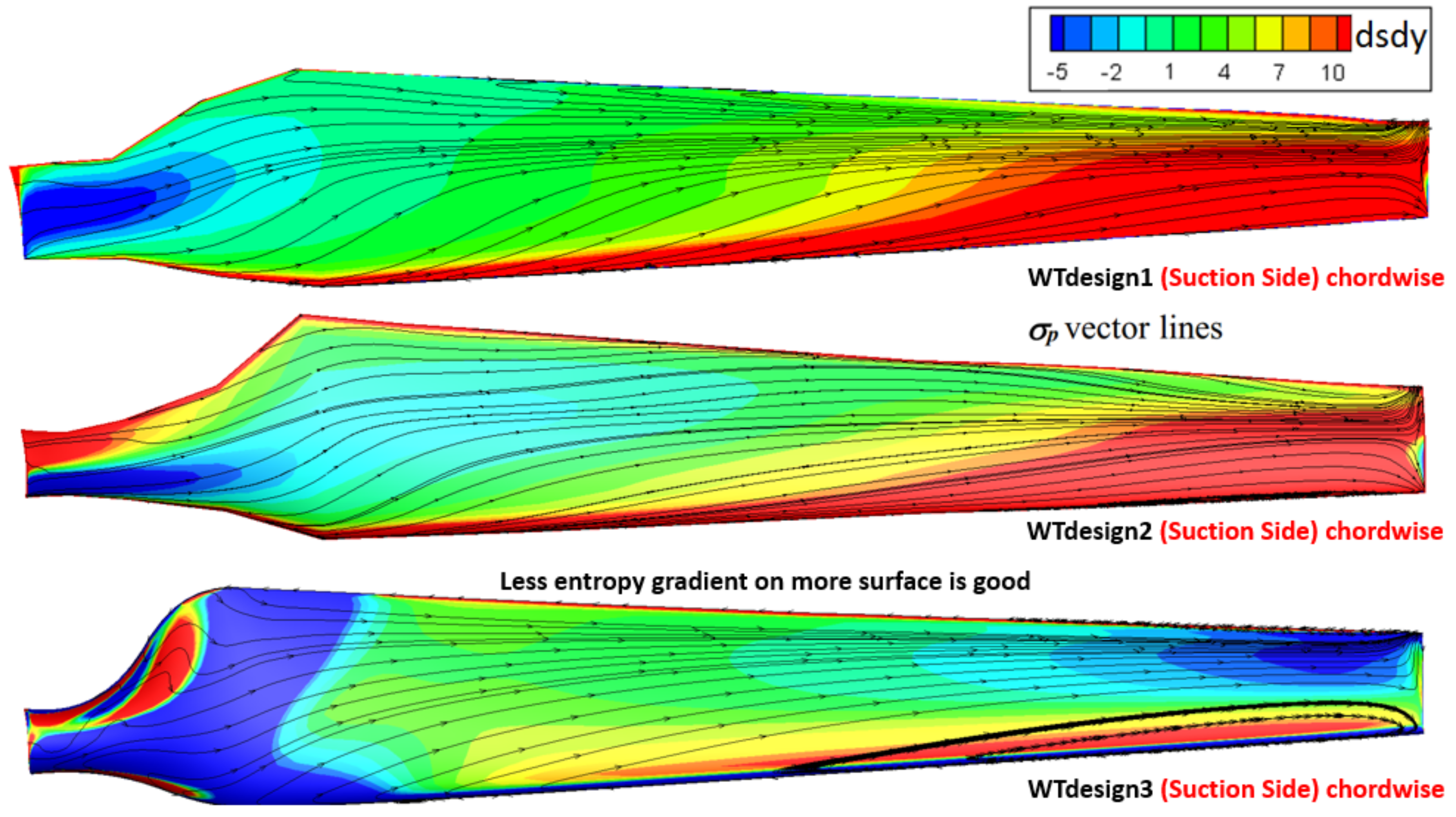
- WTdesign1: constant AoA of 8 degrees spanwise with S809 airfoil with properties from py_BEM calculation.
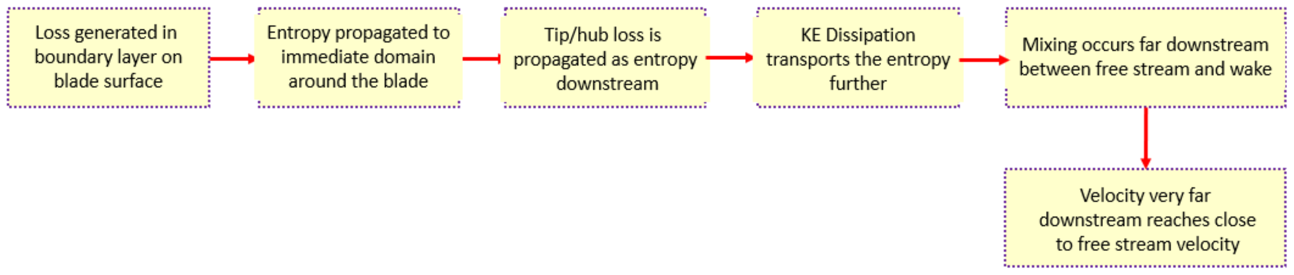
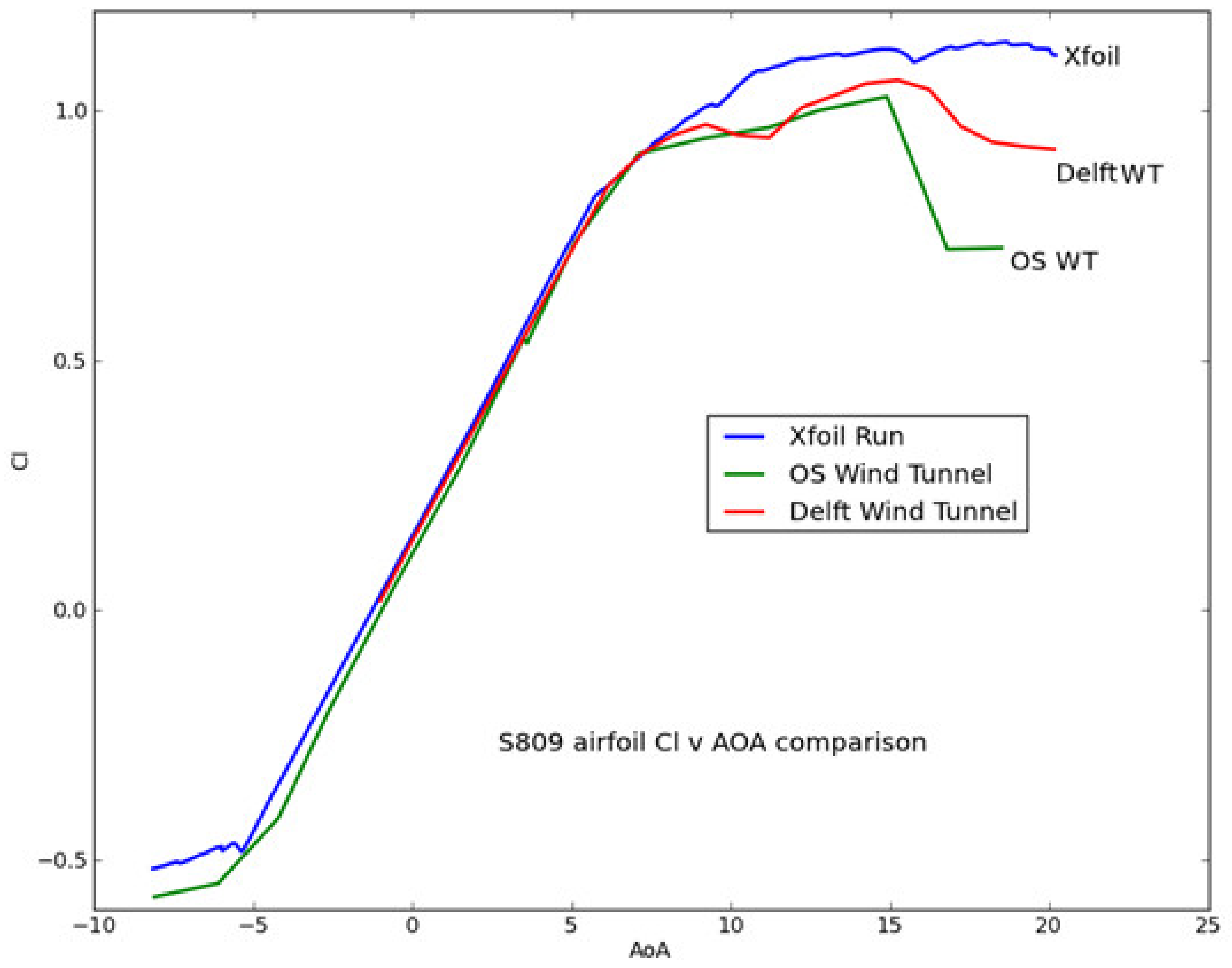
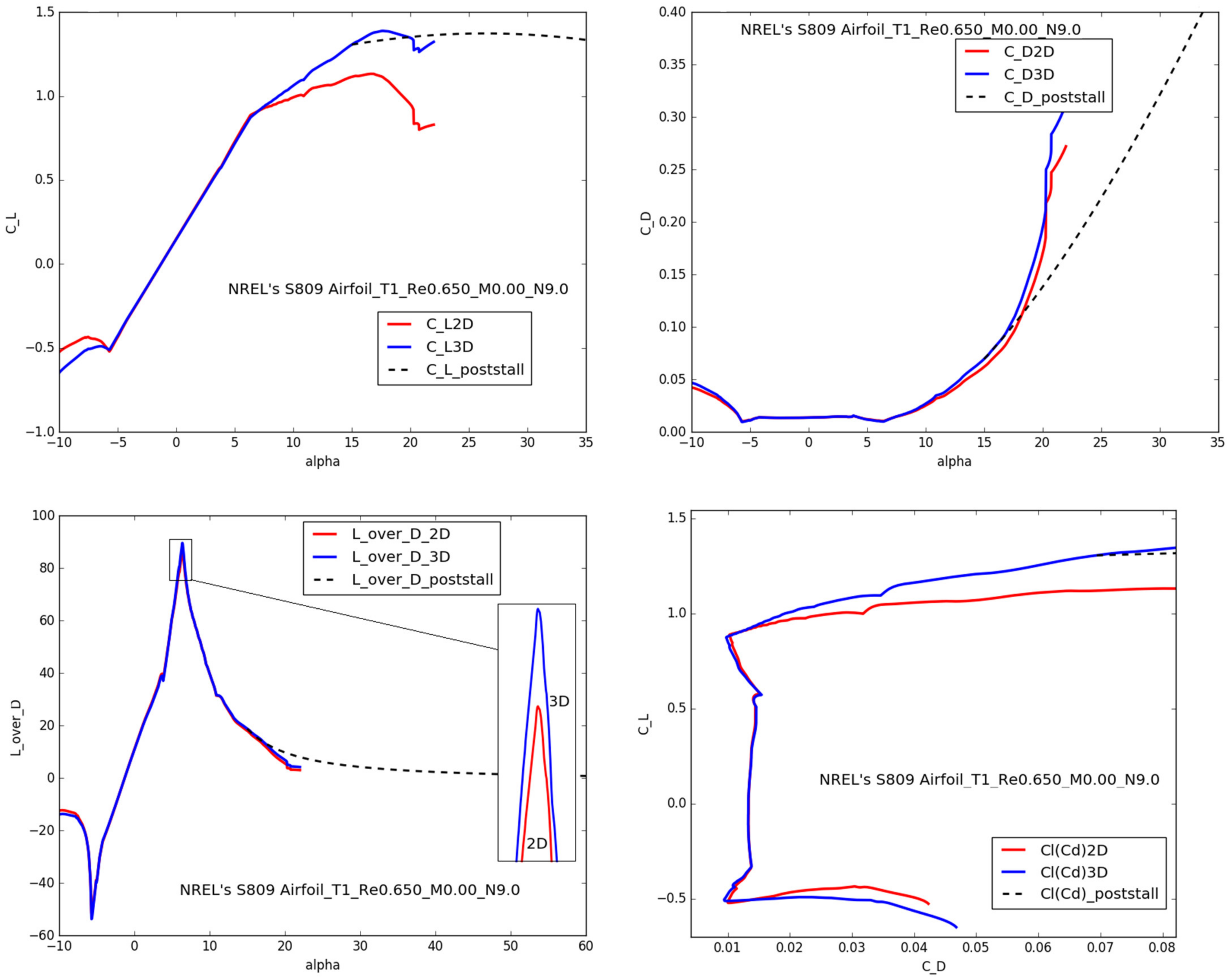
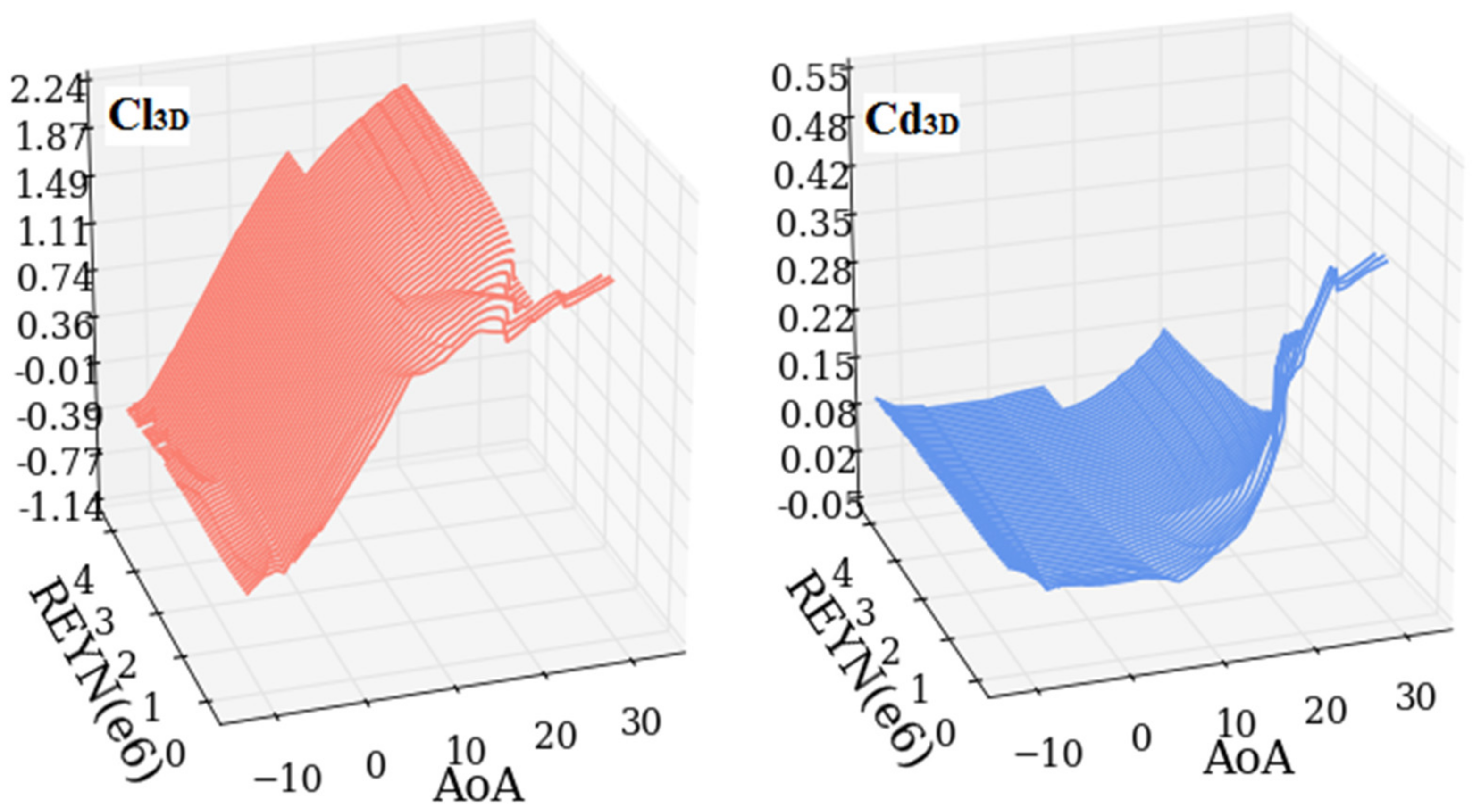
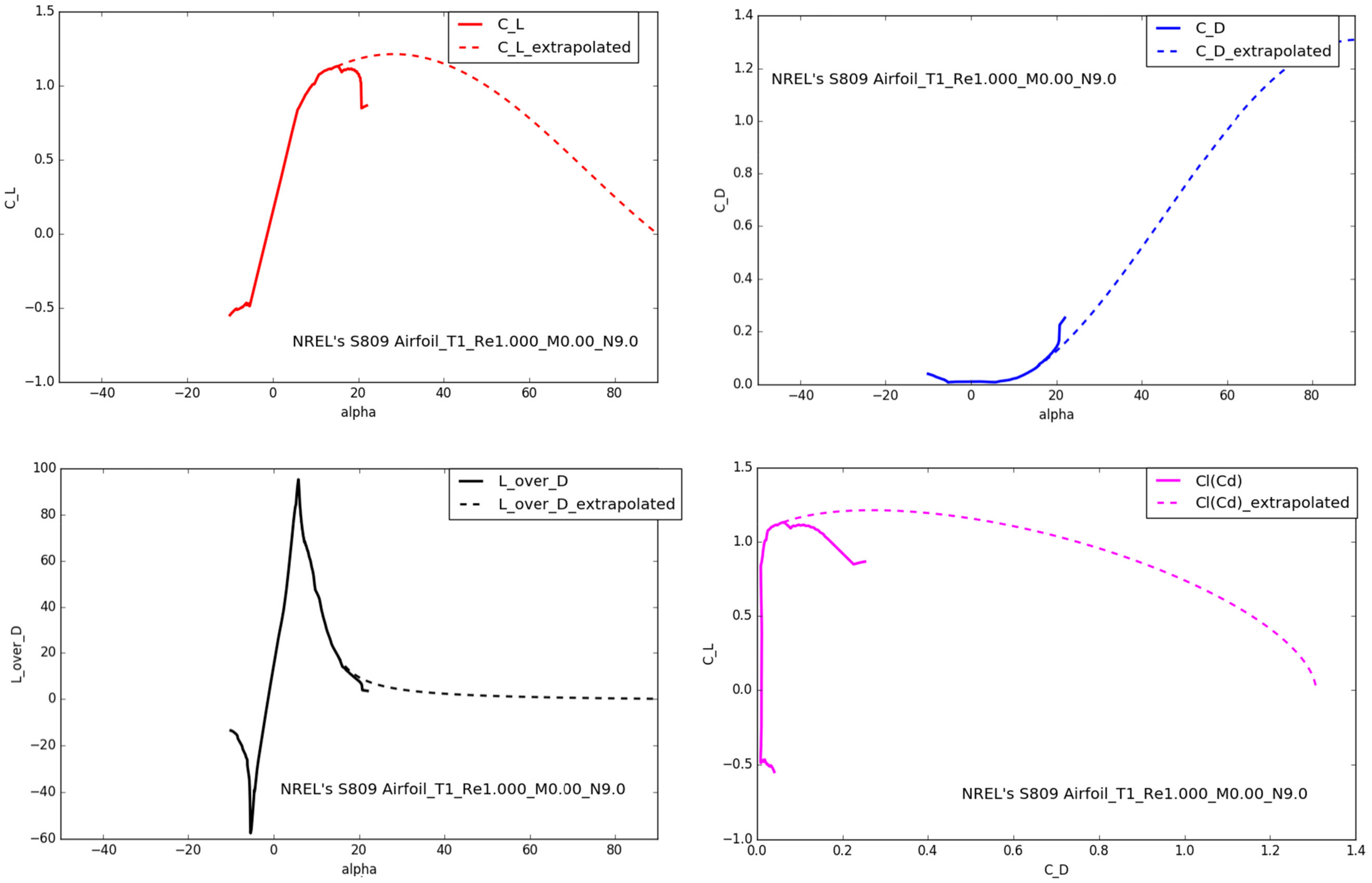
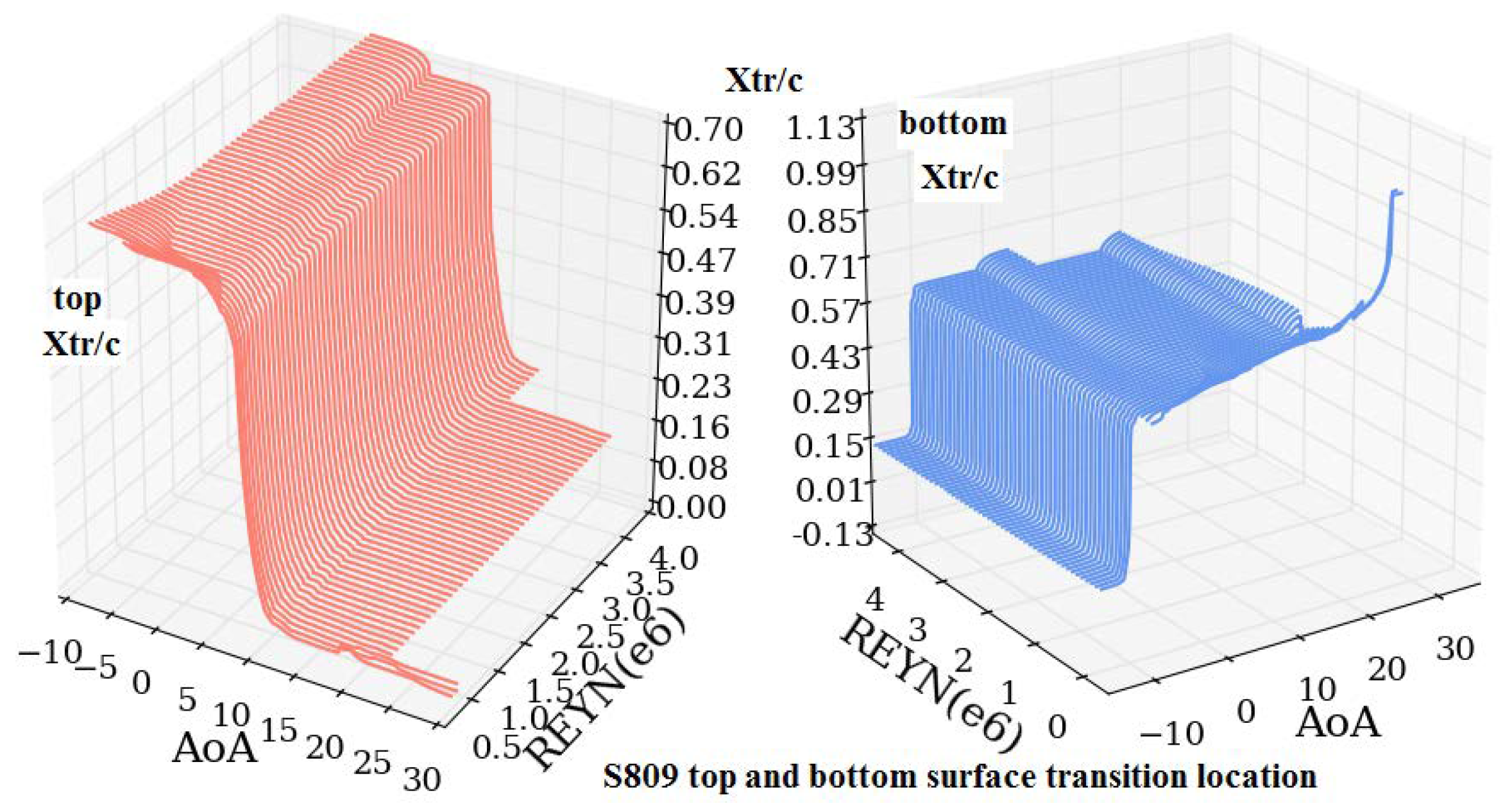
2.1. Airfoil Properties with Corrections at Low Fidelity
2.2. Low-Fidelity Design, Off-Design and Validation Using BEMT Tool
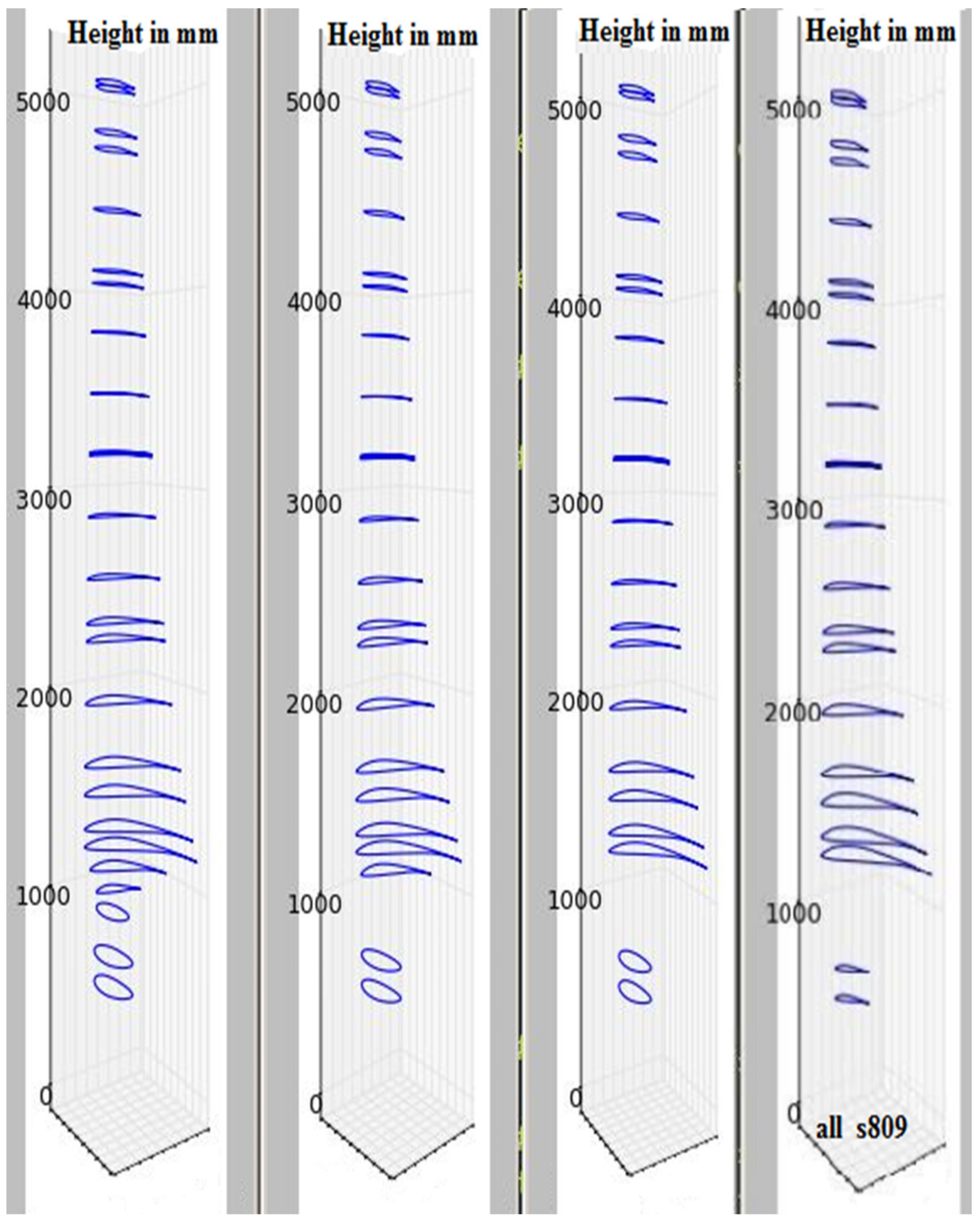
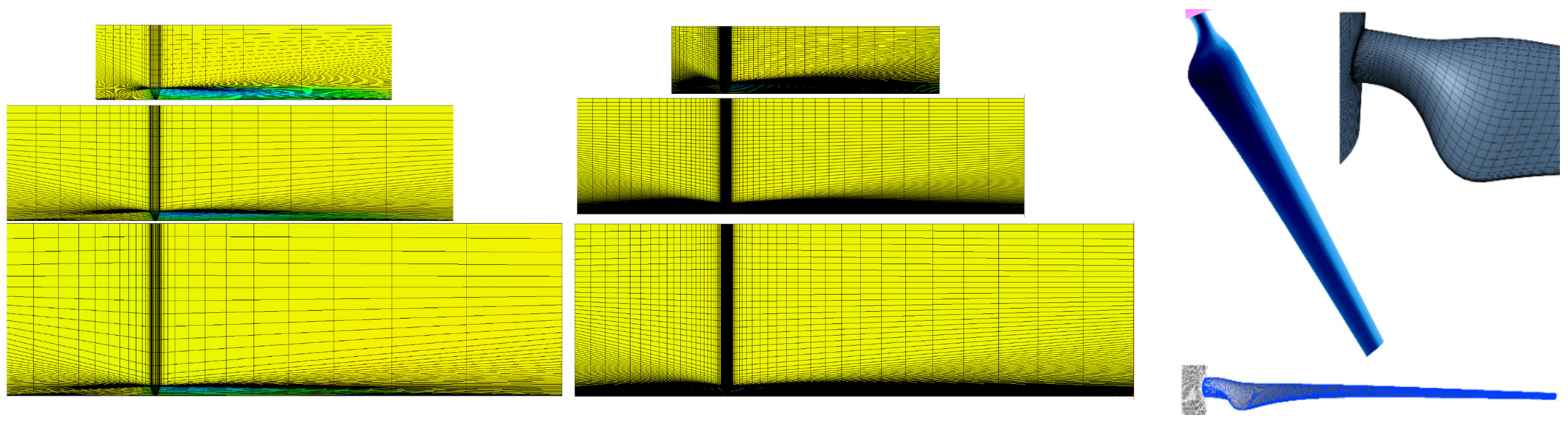
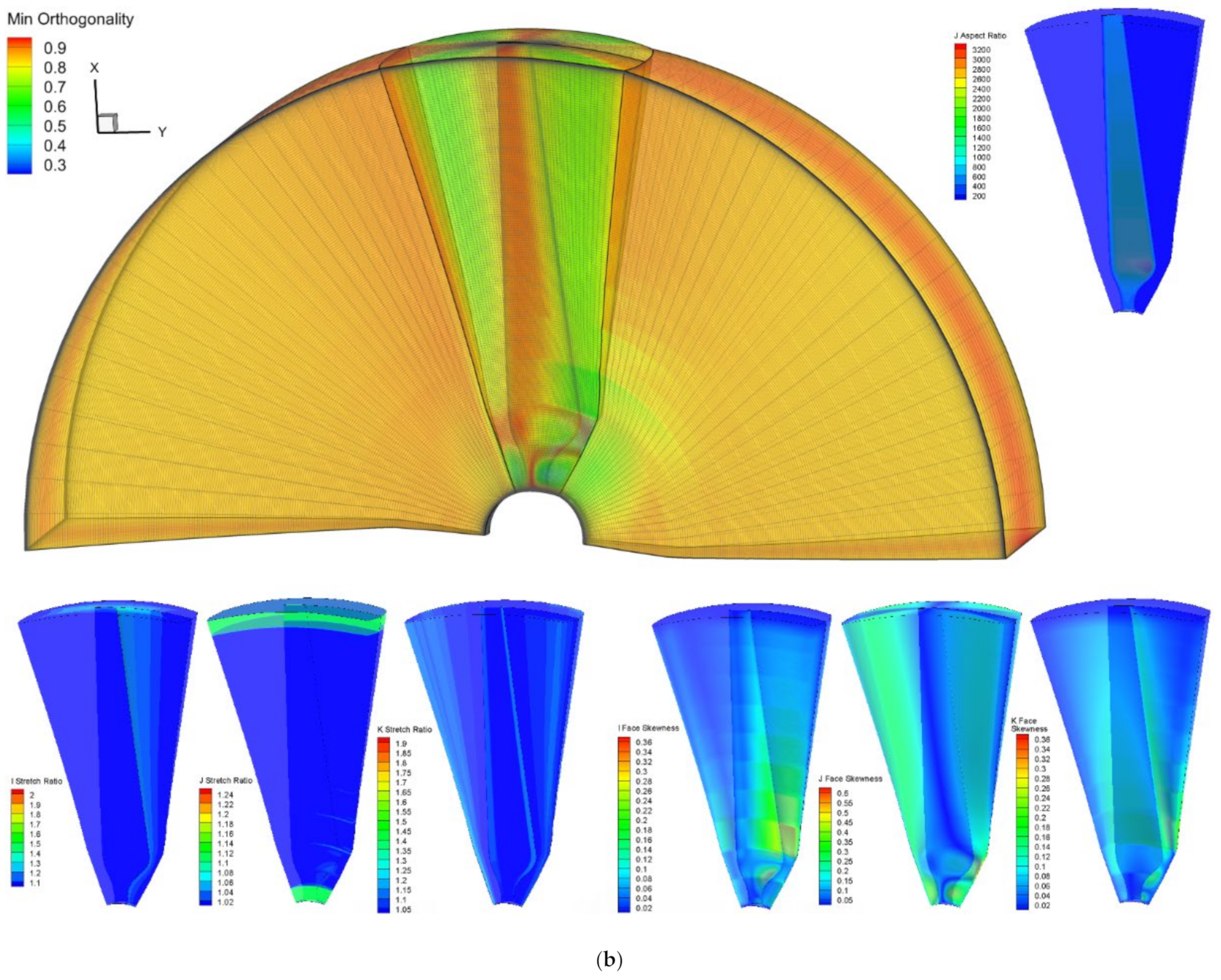
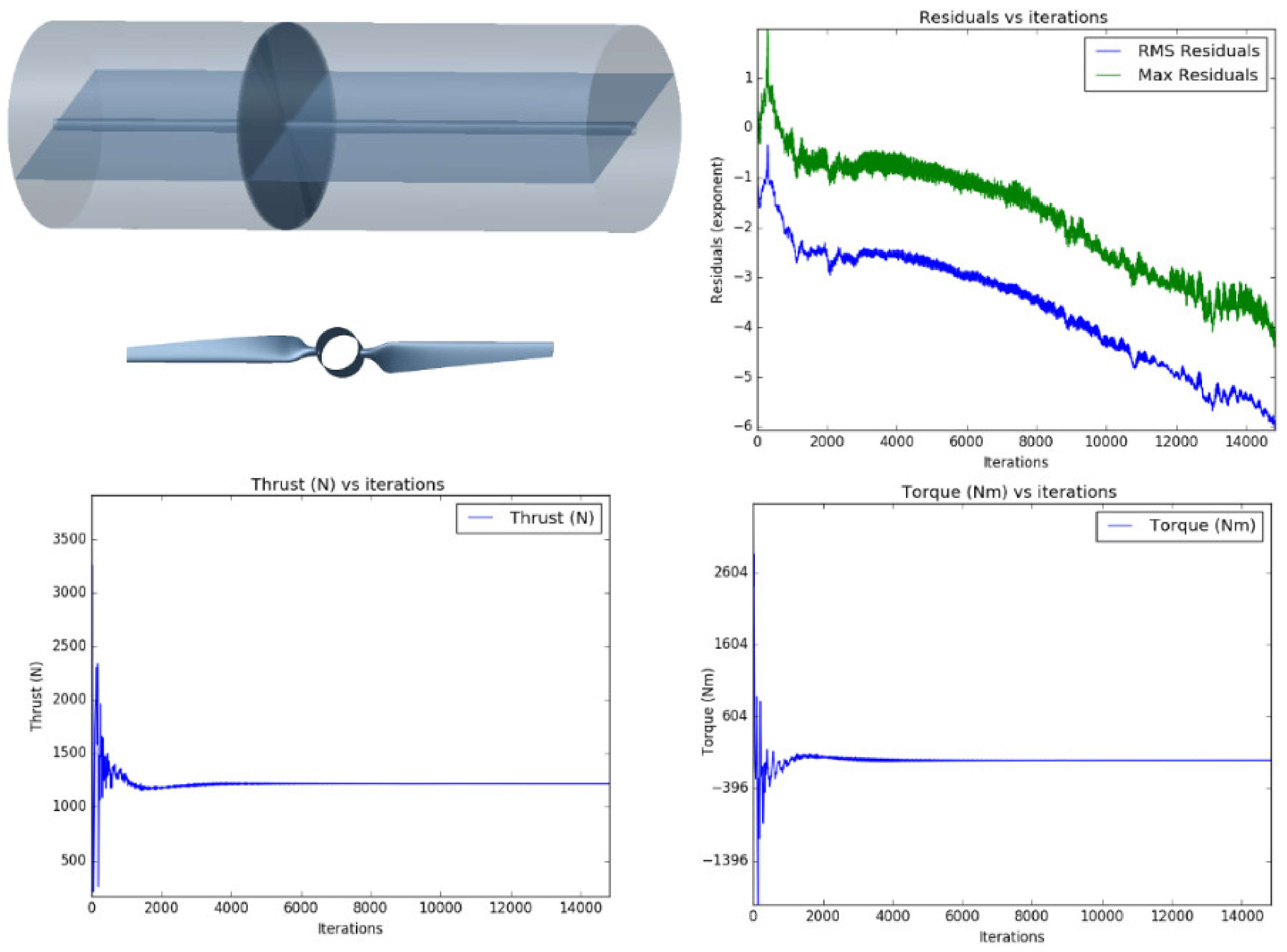
2.3. 3D Geometry and 3D Simulation Setup
3. Results
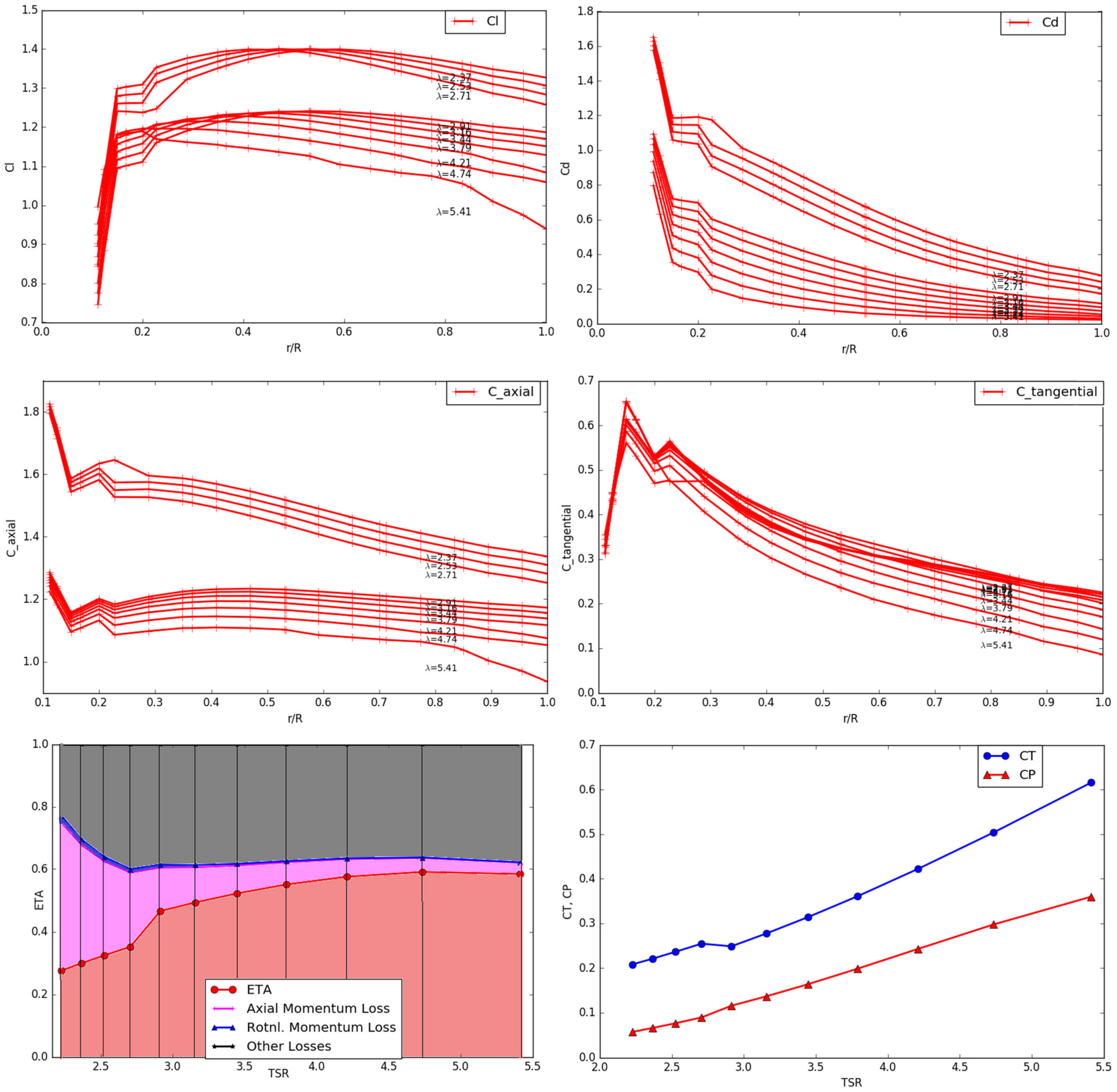
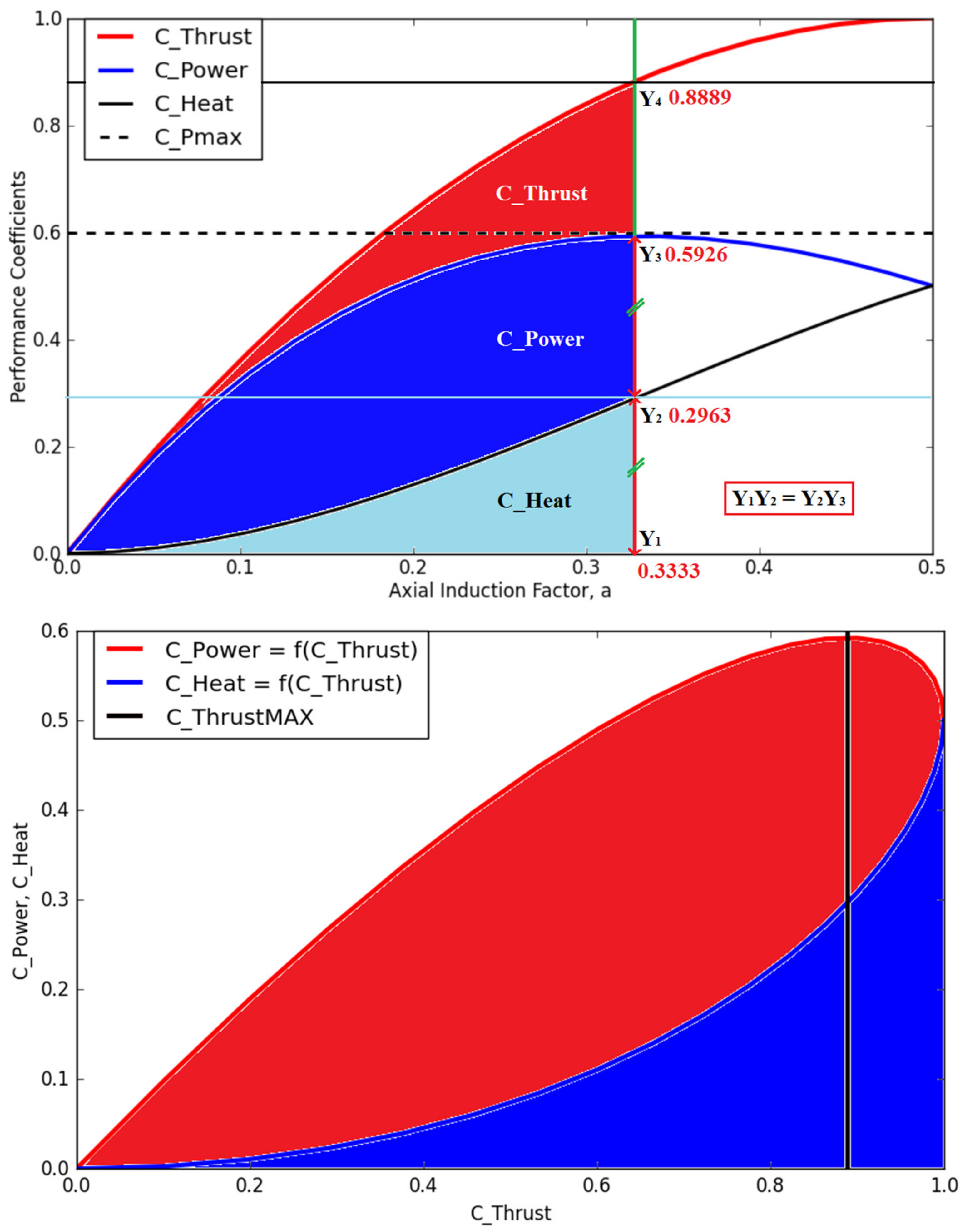
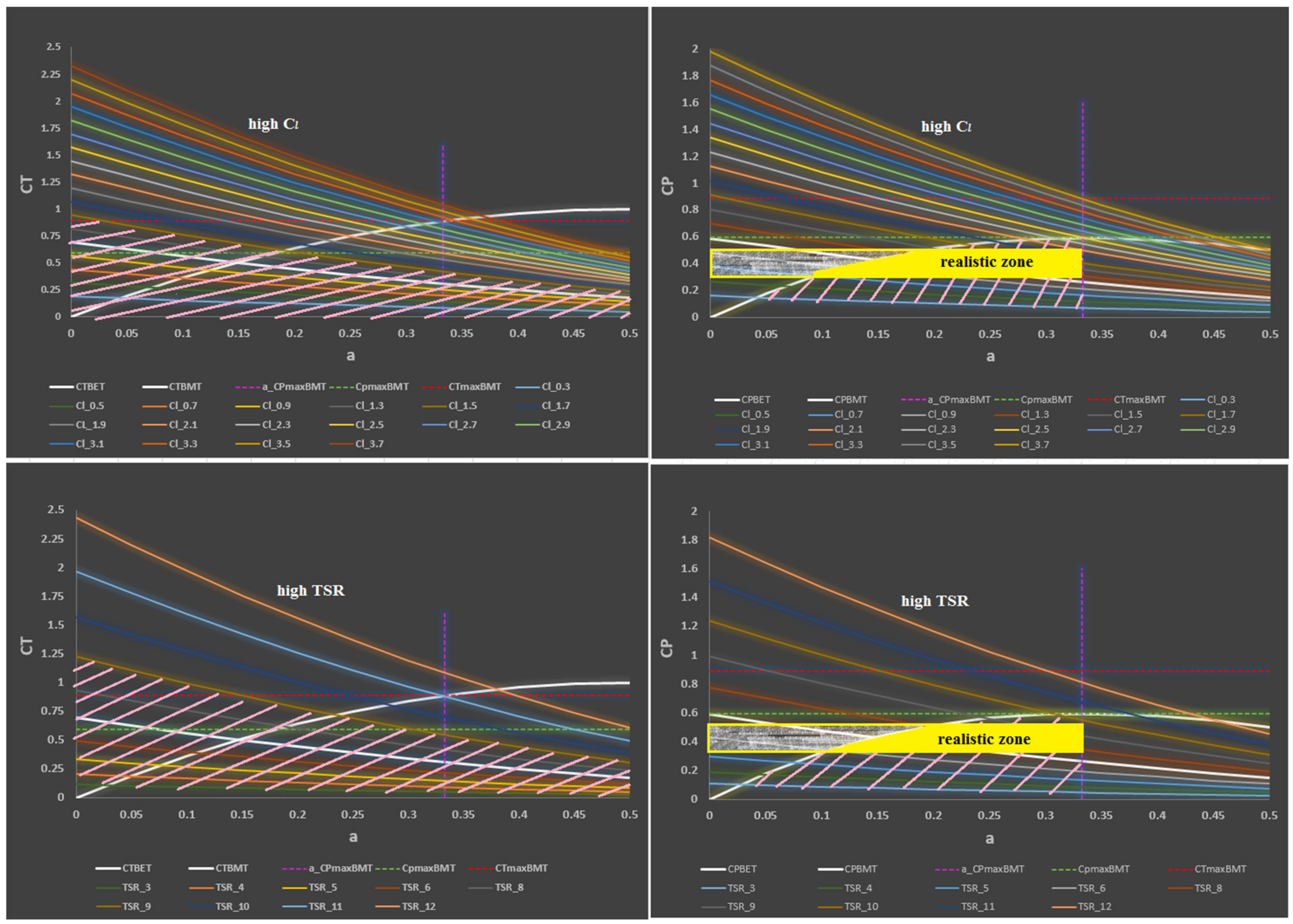
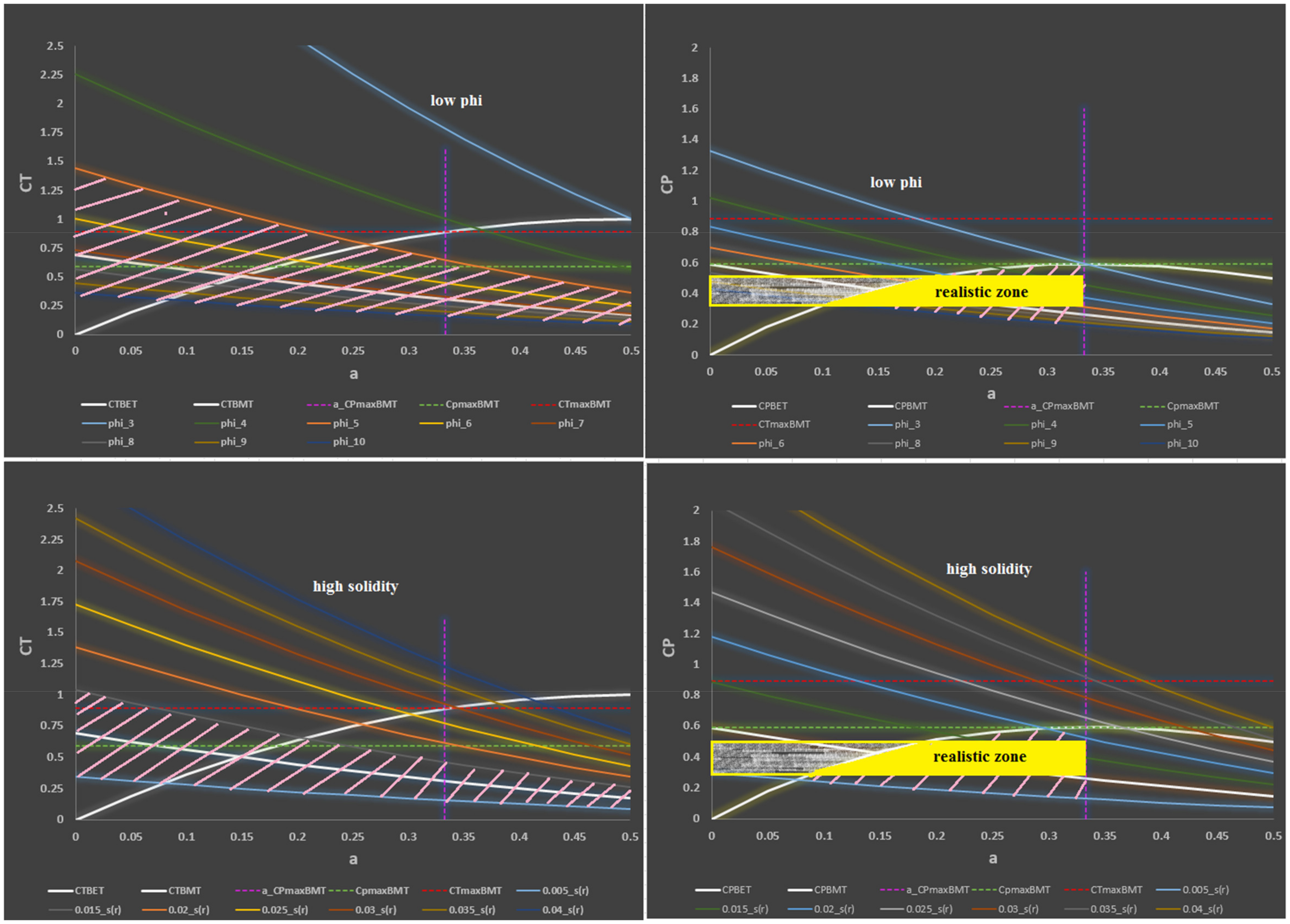
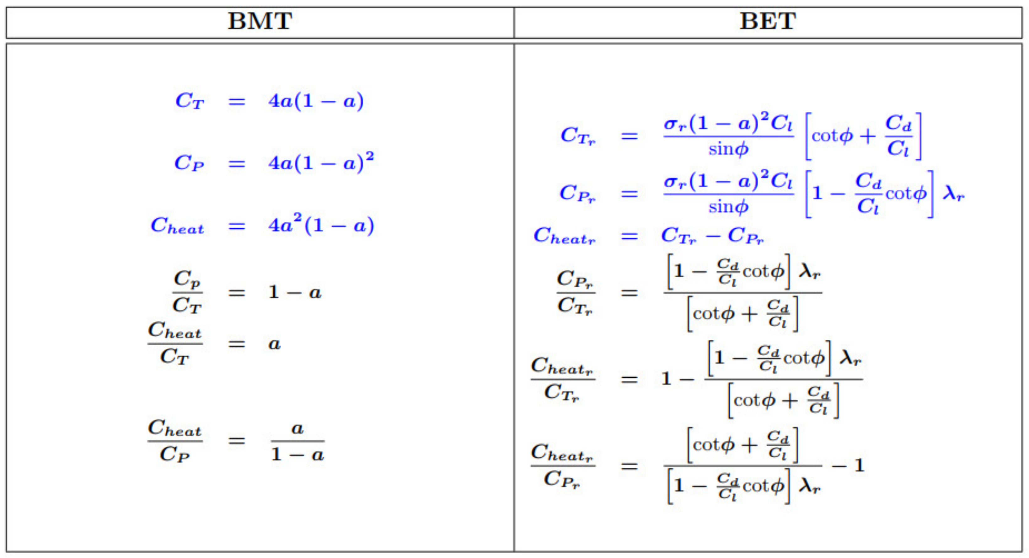
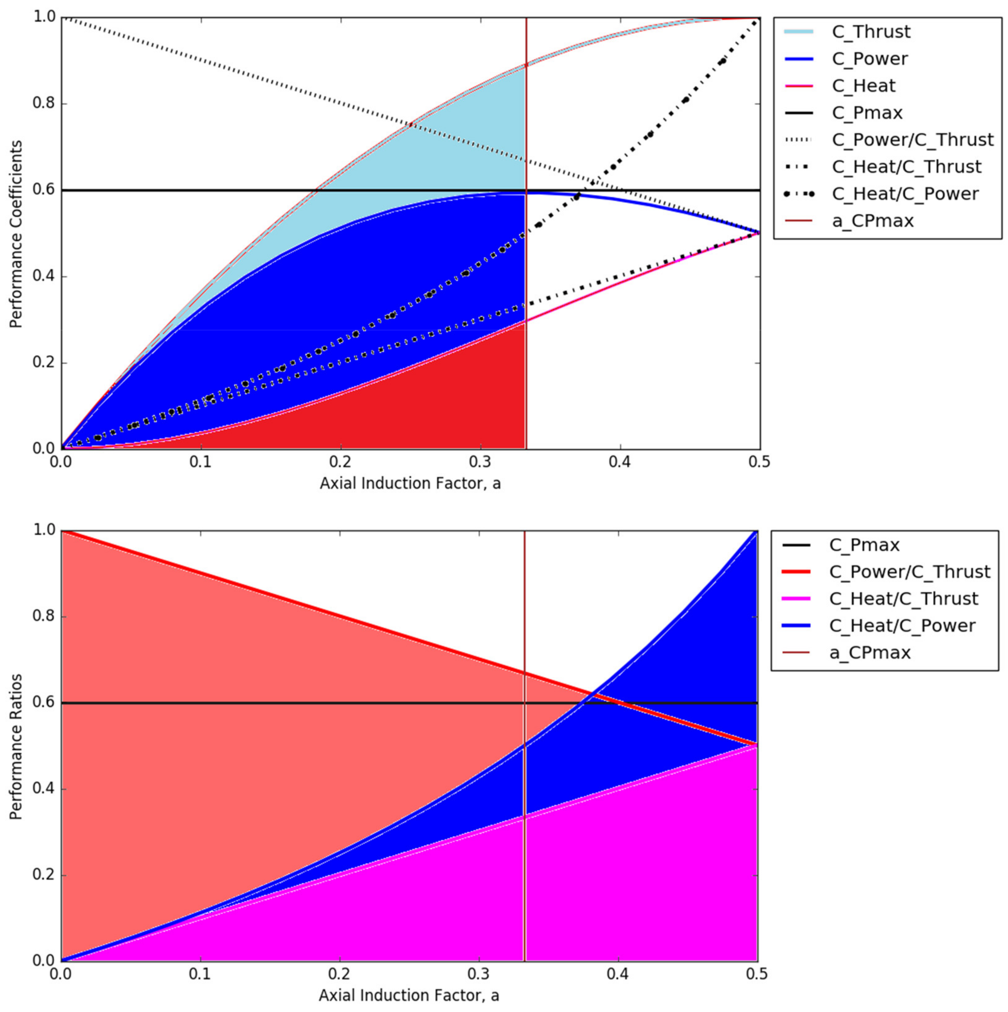
3.1. Realistic Coefficients of Thrust and Power
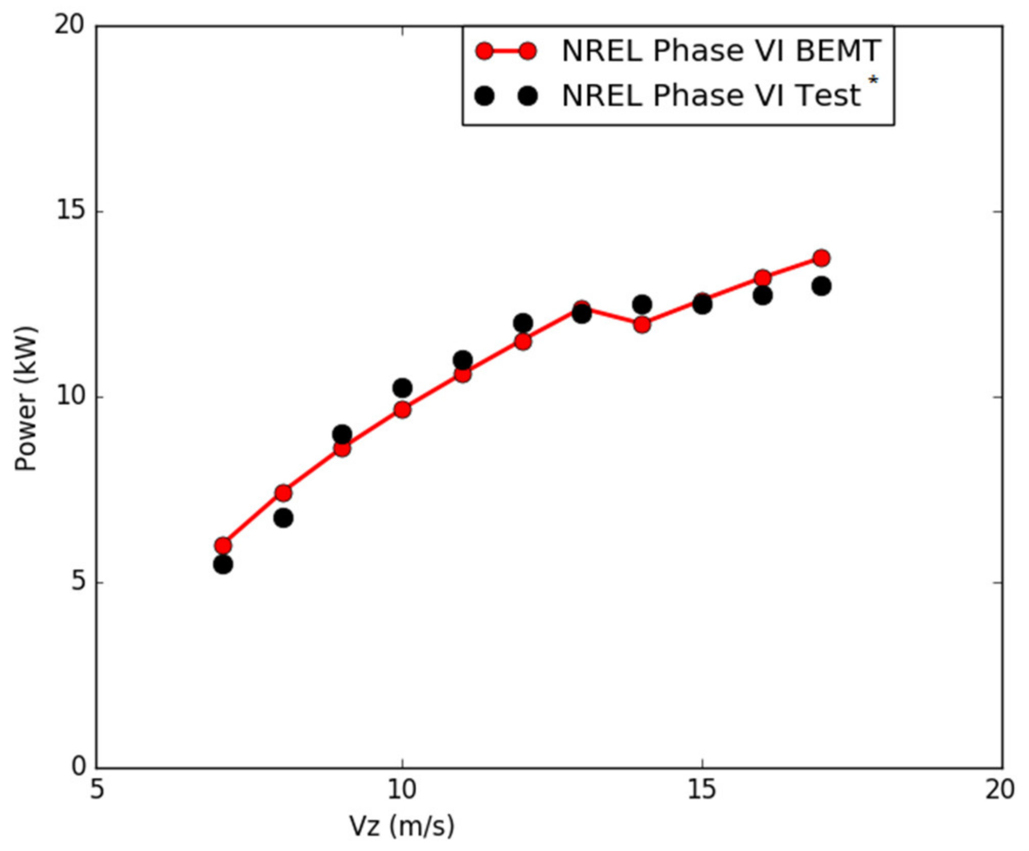
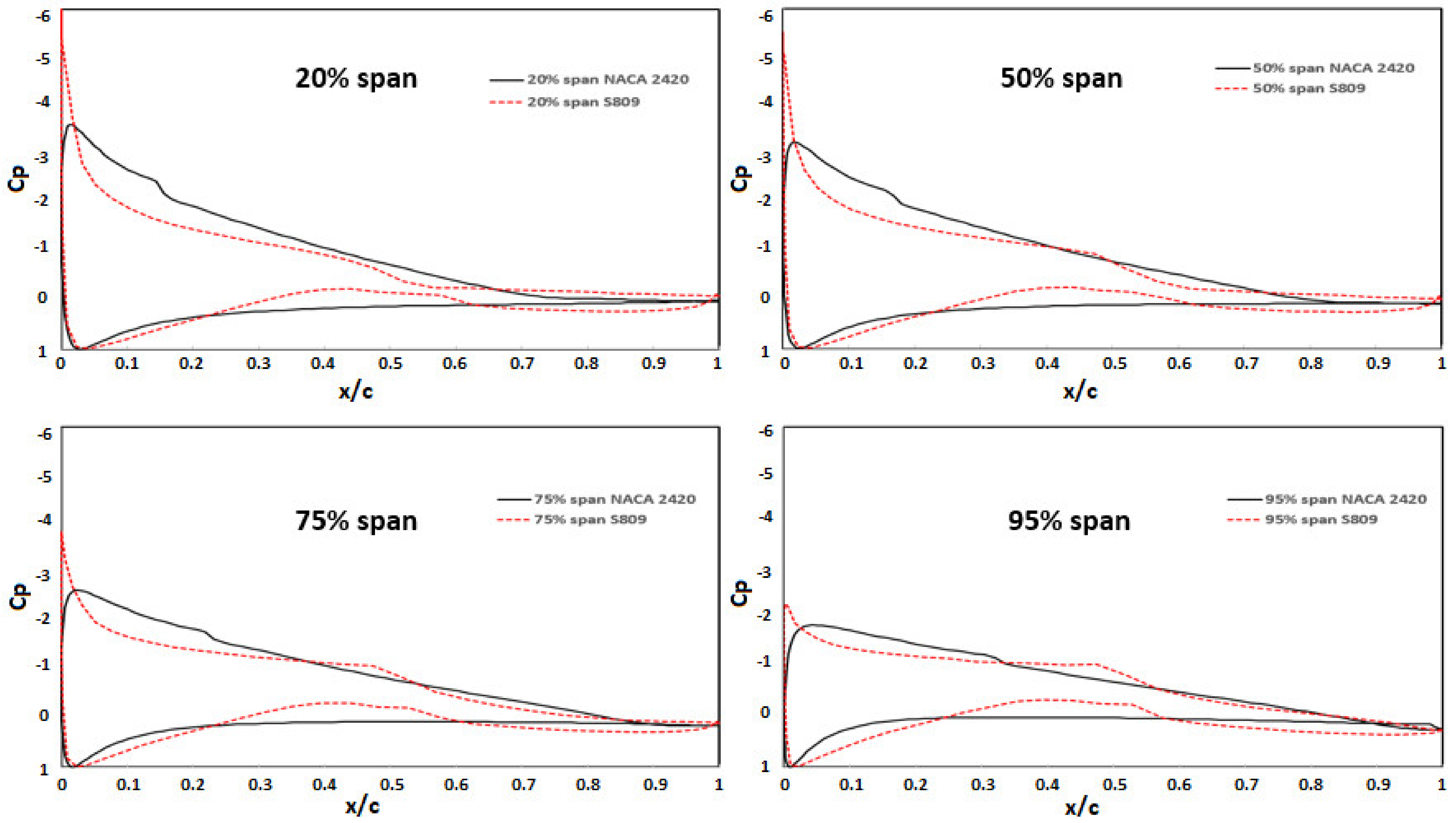
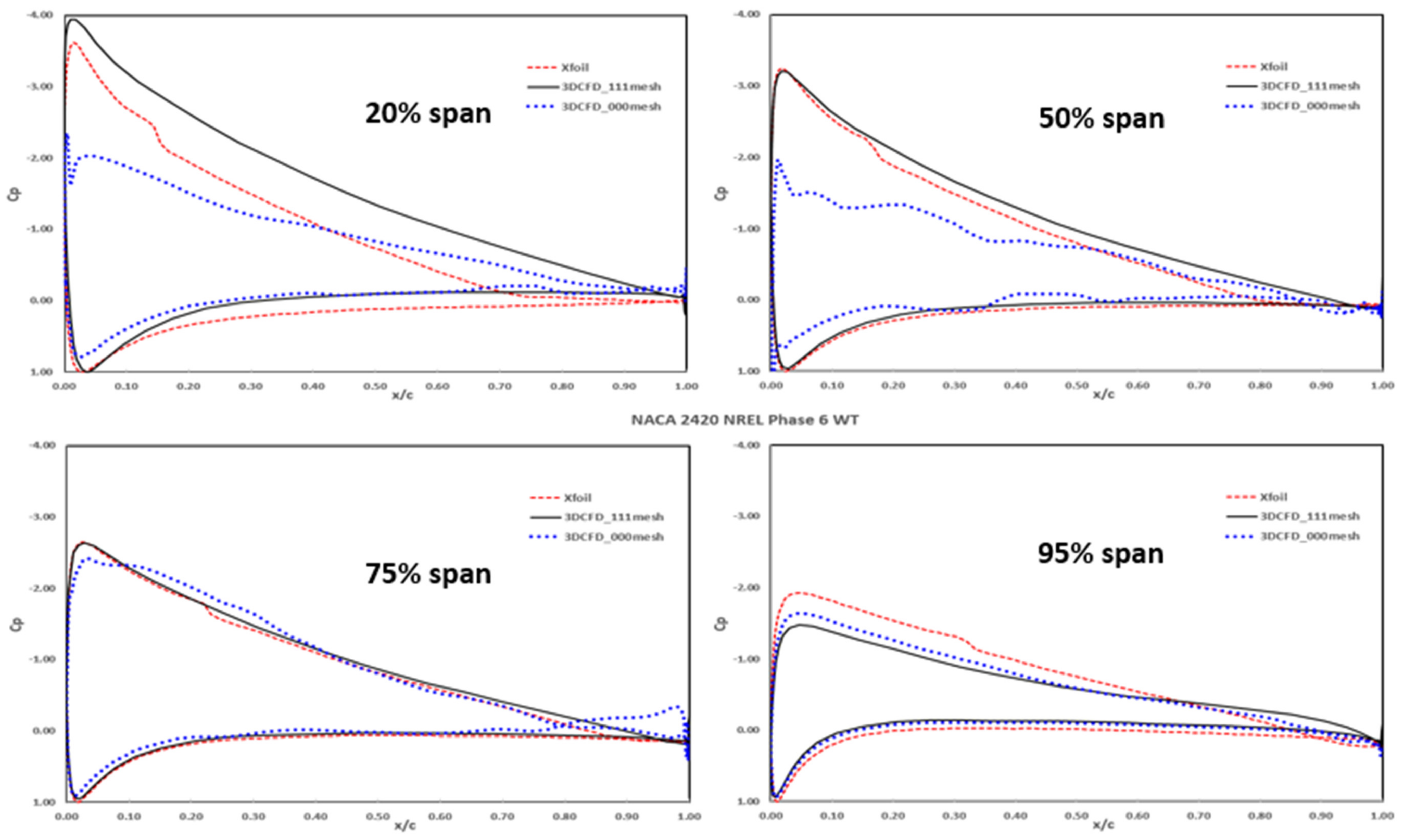
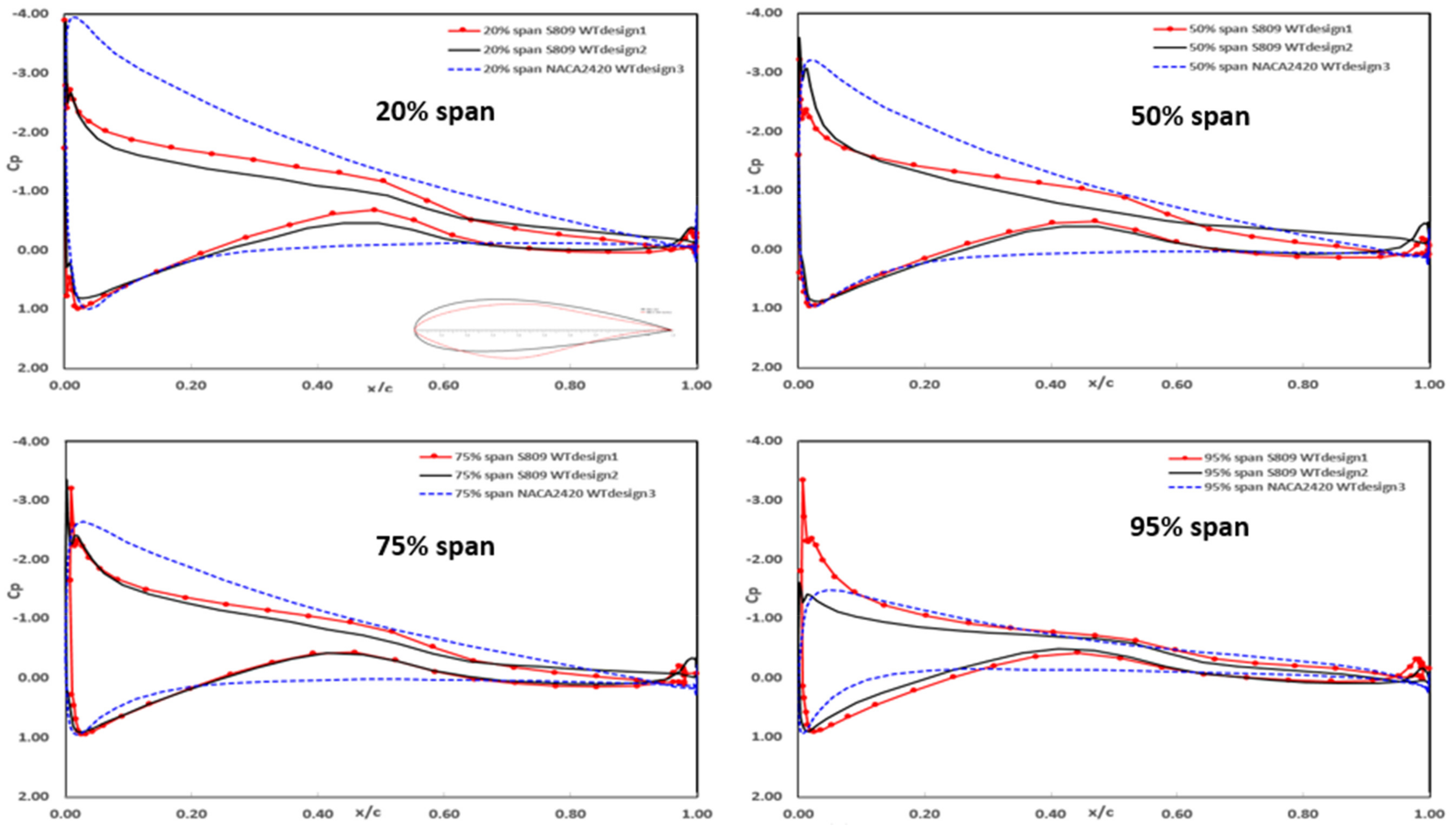
3.2. Comparison between Low and High Fidelity
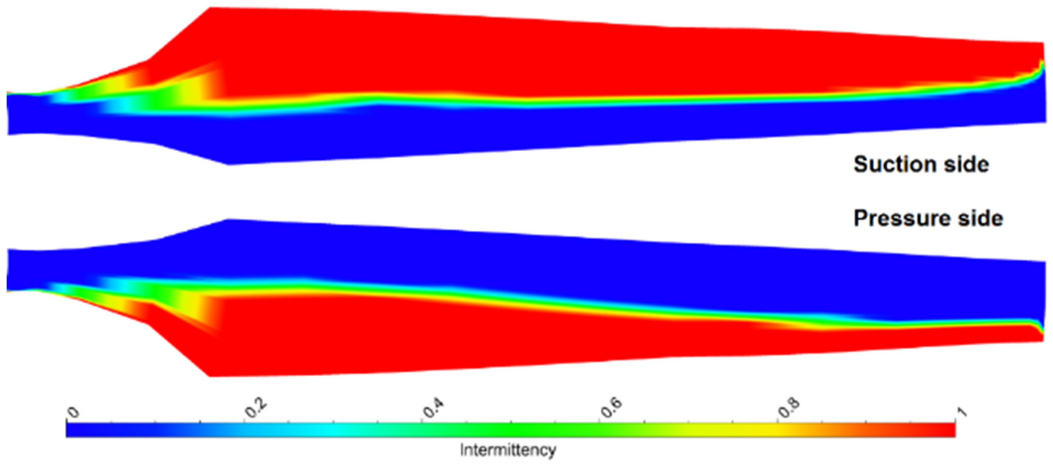
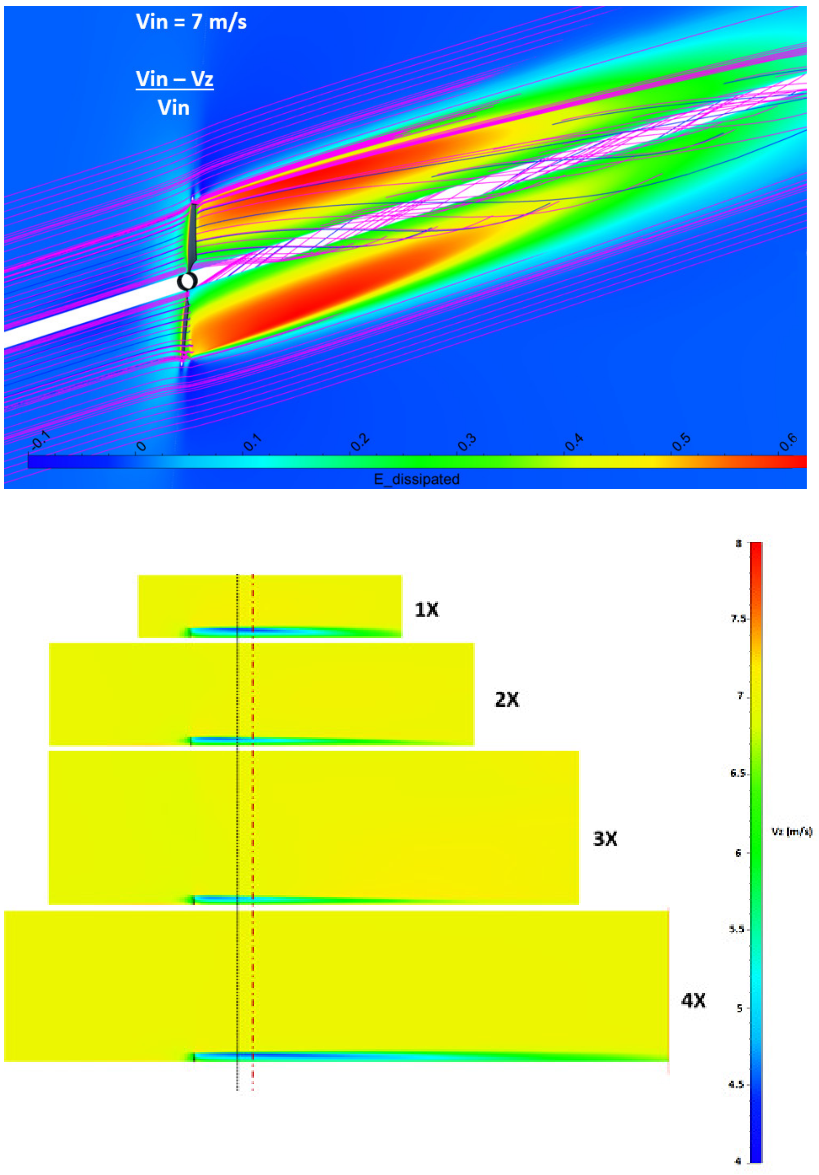
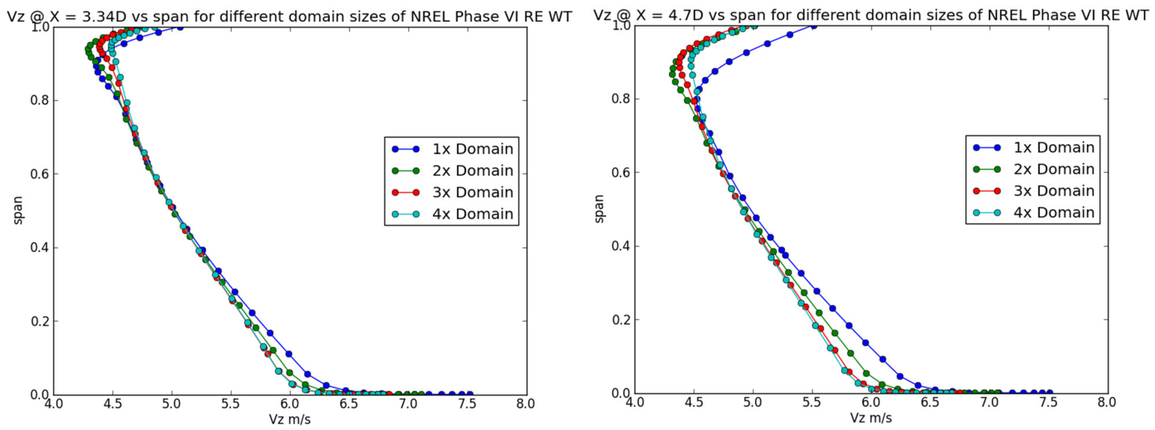
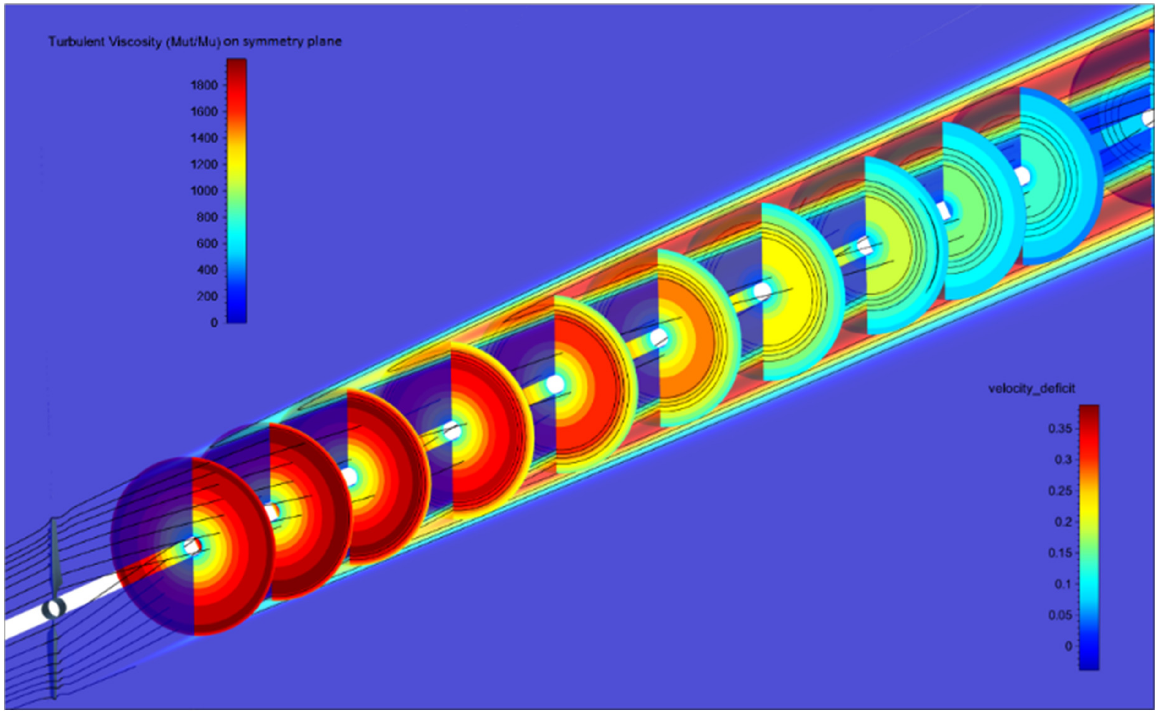
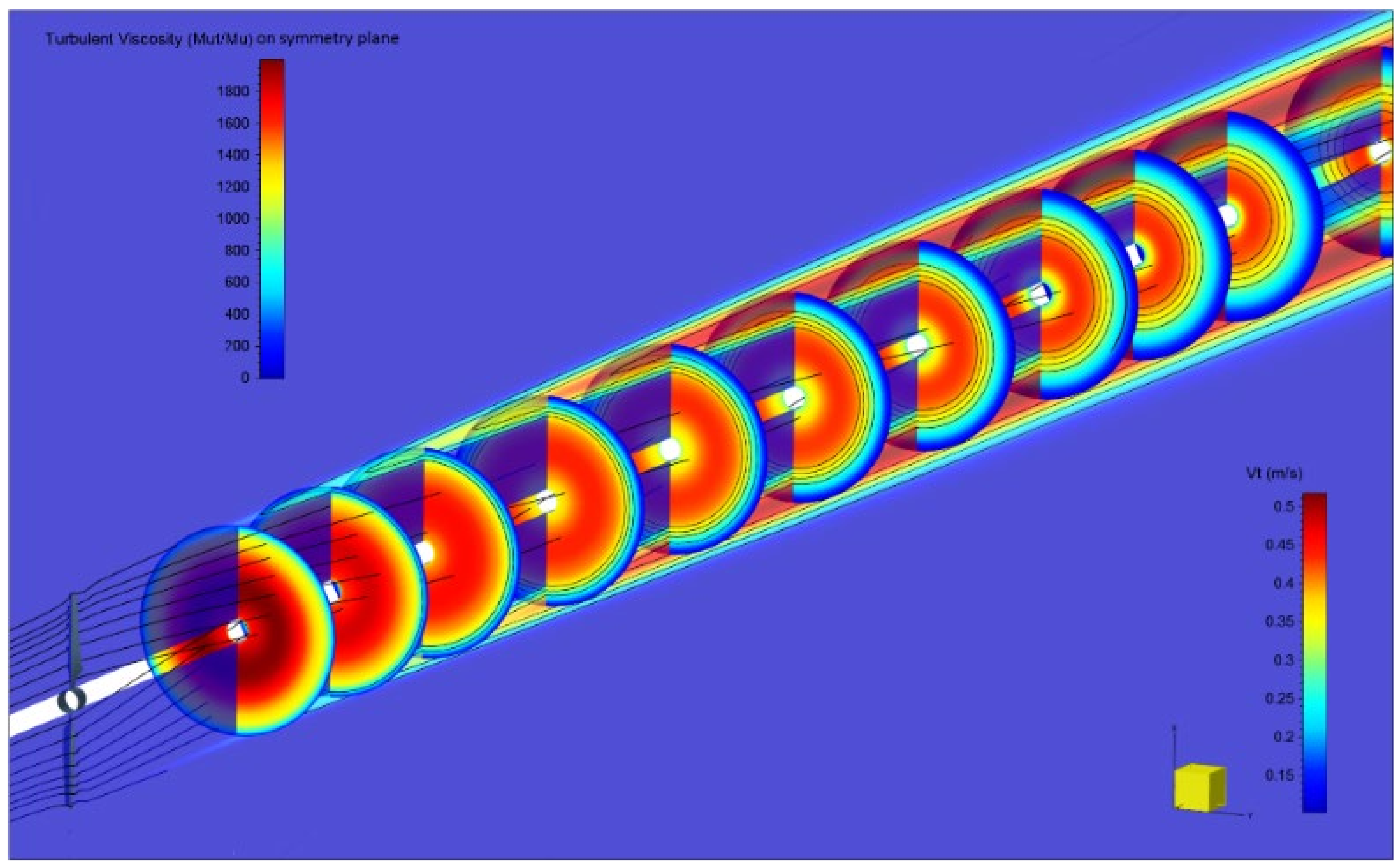
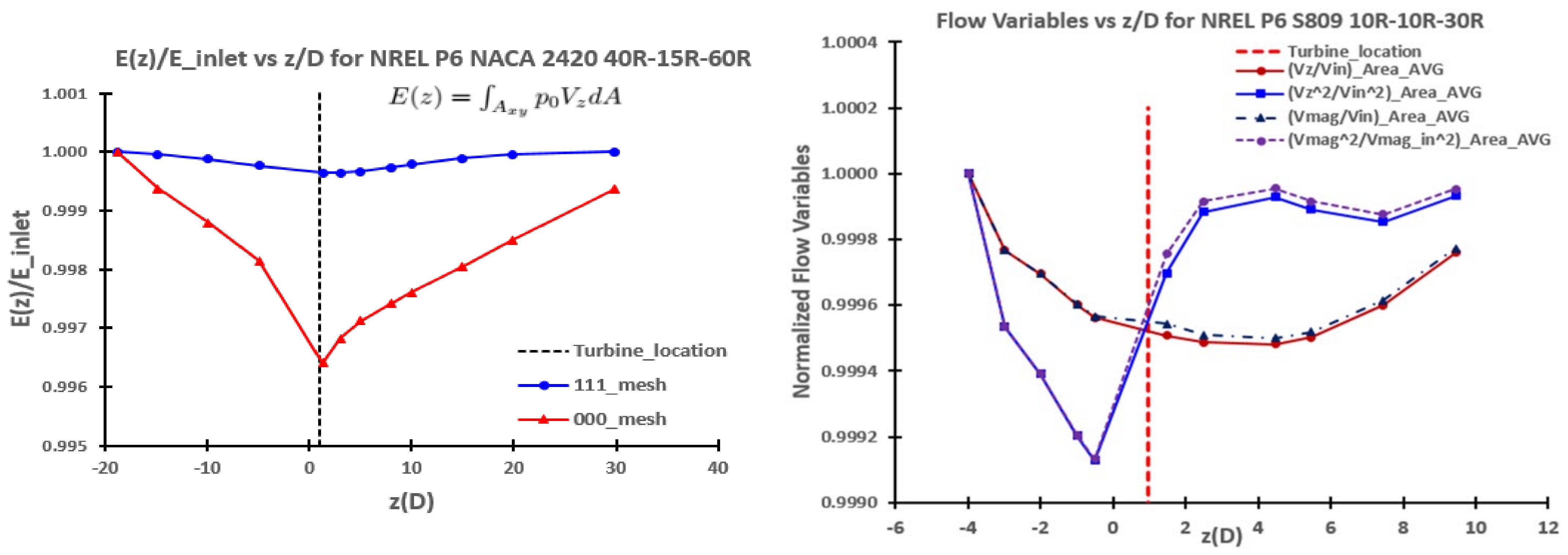
3.3. Momentum Transport and Wake Analysis
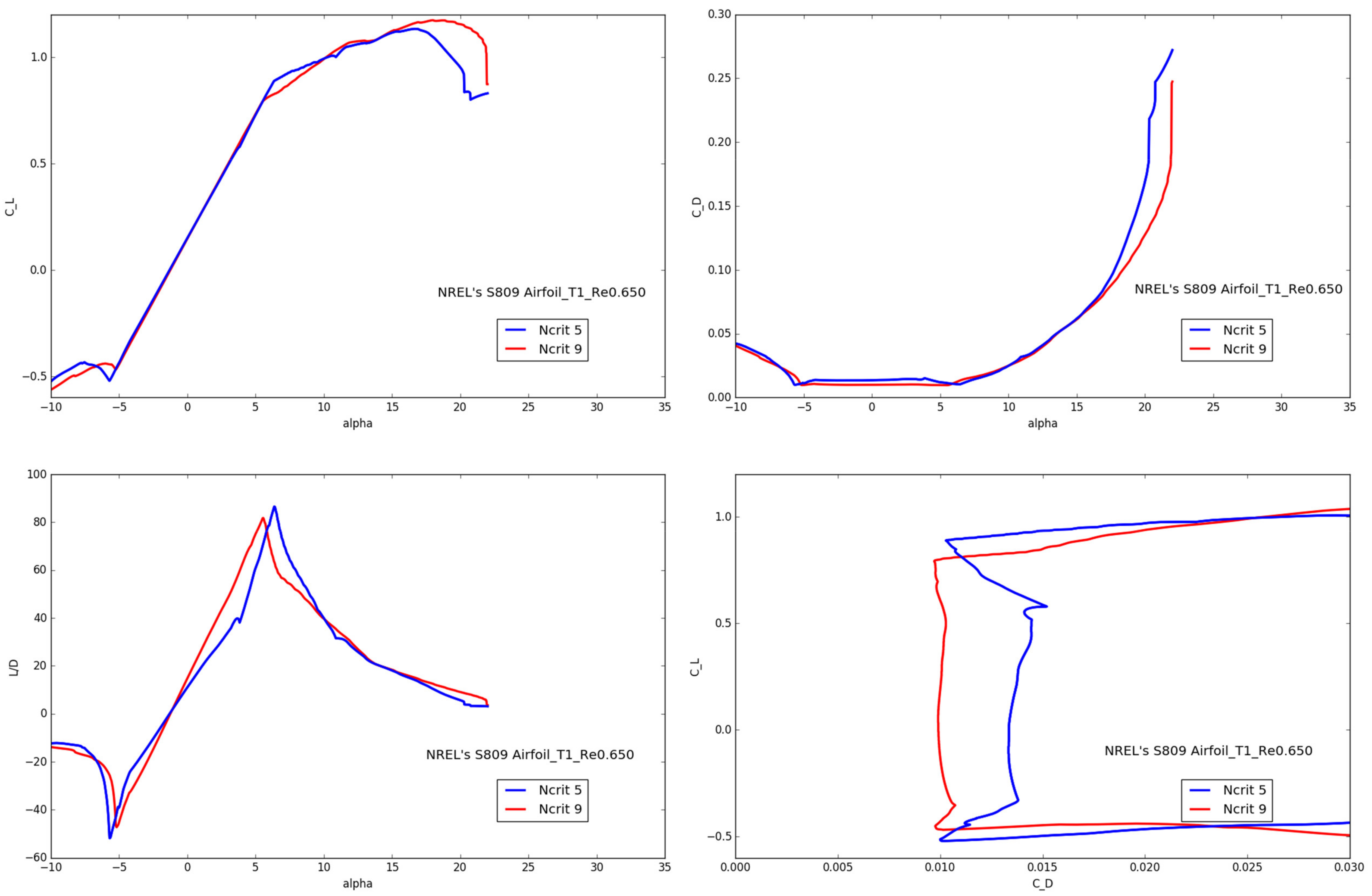
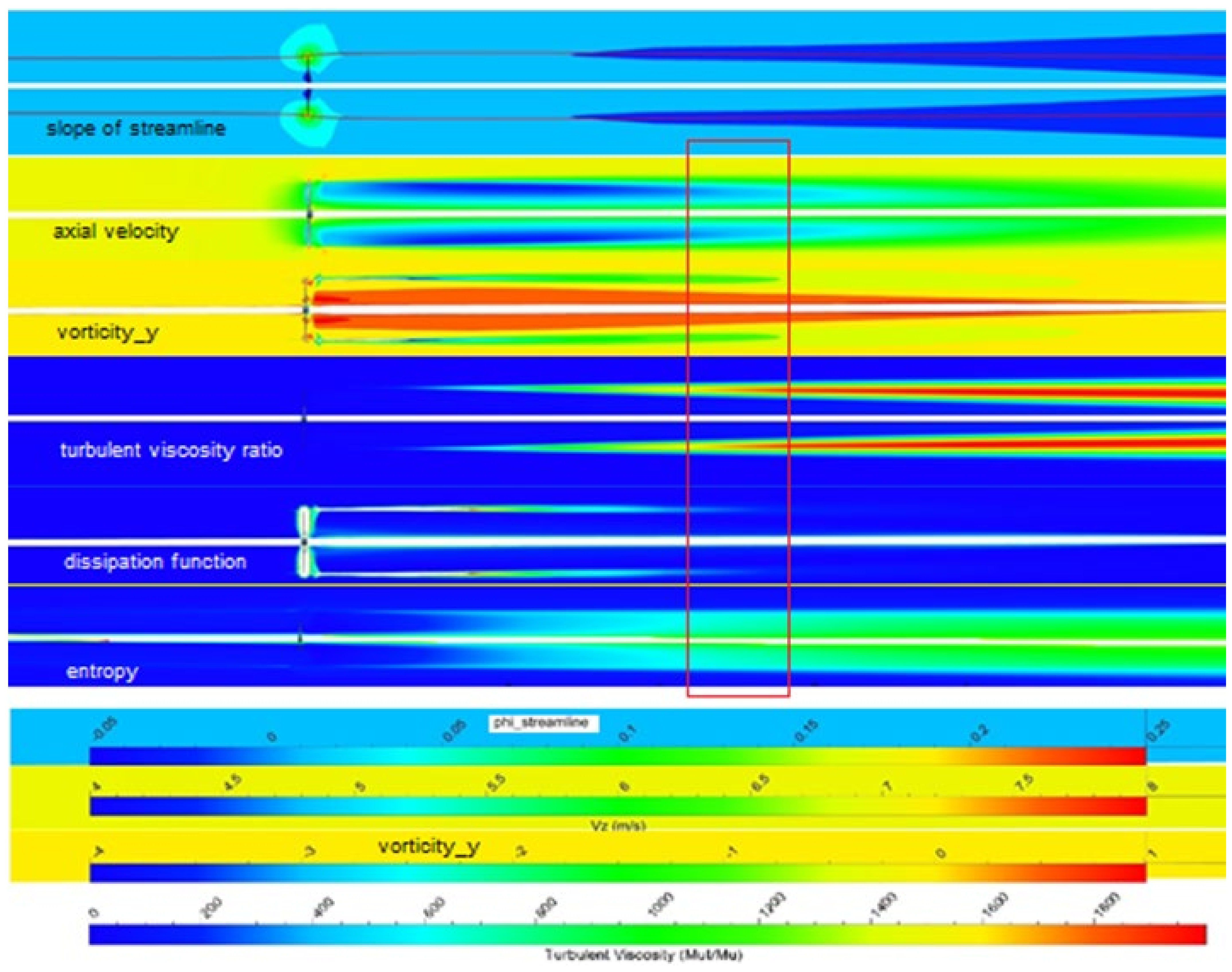
3.4. Vorticity Dynamics and Entropy Increase
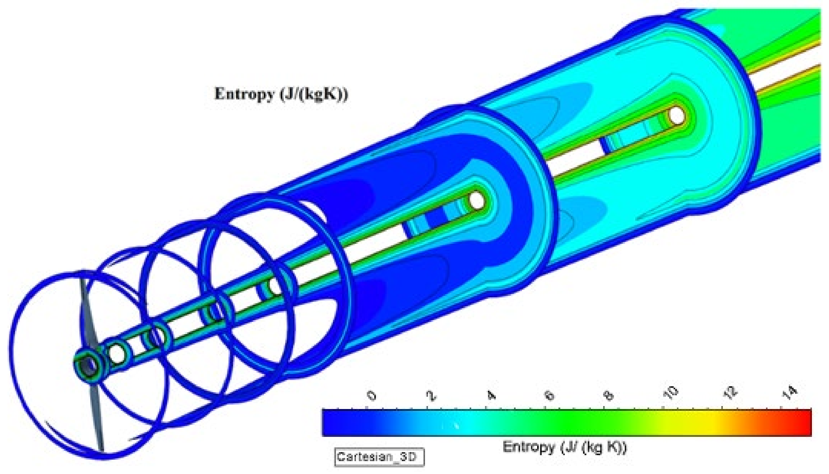
3.5. Kinetic Energy Dissipation as Entropy Rise
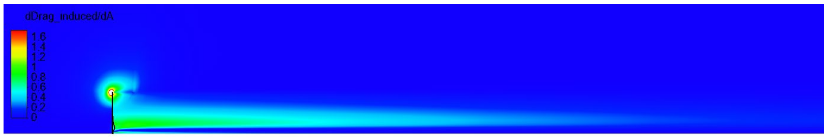
3.6. Drag as a Form of Entropy
3.7. Rothalpy and Viscous Power Loss
4. Conclusions
Author Contributions
Funding
Institutional Review Board Statement
Informed Consent Statement
Acknowledgments
Conflicts of Interest
Nomenclature
| a, a′ | Axial and angular induction factors |
| Cl, Cd | Coefficient of lift and drag |
| CT, CP | Coefficient of thrust and power |
| dF, D, L | Elemental force, drag, lift |
| f | Frictional |
| h | Enthalpy |
| I | Rothalpy |
| m | Mass flow |
| p, P | Pressure, Power |
| U | Rotational Velocity |
| V | Absolute Velocity |
| W | Relative Velocity |
| s | Entropy |
| y+ | Non-dimensional wall distance |
| α | Angle of Attack |
| μ | Dynamic viscosity |
| υ | Kinematic viscosity |
| Ω | Rotational speed of the rotor |
| ω | Vorticity vector, angular velocity |
| φ, Φ | Flow angle, streamline slope, dissipation function |
| ρ | Fluid Density |
| σ | Boundary vorticity flux |
| τ | Skin friction vector |
| θ | Twist angle, tangential direction |
References
- Wilson, R.E.; Lissaman, P.B.S. Applied Aerodynamics of Wind-Power Machines; NTIS: Alexandra, VI, USA, 1974. [Google Scholar]
- Manwell, J.F.; McGowan, J.G.; Rogers, A.L. Wind Energy Explained: Theory, Design and Application, 1st ed.; J.W & Sons, Inc.: Middle River, MD, USA, 2002. [Google Scholar]
- Gundtoft, S. Wind Turbines; University College of Aarhus: Aarhus, Denmark, 2009. [Google Scholar]
- Masters, I.; Chapman, J.C.; Wills, M.R.; Orme, J. A robust blade element momentum theory model for tidal stream turbines including tip and hub loss corrections. J. Mar. Eng. Technol. 2011, 10, 25–35. [Google Scholar] [CrossRef] [Green Version]
- Masters, I.; Chapman, J.C.; Orme, J.; Wills, M.R. Modelling high axial induction flows in tidal stream turbines with a corrected blade element model. In Proceedings of the 3rd International Conference on Ocean Energy, Bilbao, Spain, 6–9 October 2010. [Google Scholar]
- Ingram, G. Wind Turbine Blade Analysis Using the Blade Element Momentum Method Version 1.1; Durham University: Durham, UK, 2011. [Google Scholar]
- Liu, S.; Janajreh, I. Development and application of an improved blade element momentum method model on horizontal axis wind turbines. Int. J. Energy Environ. Eng. 2012, 3, 30. [Google Scholar] [CrossRef] [Green Version]
- Stępień, M.; Kulak, M.; Jóźwik, K. “Fast Track” Analysis of Small Wind Turbine Blade Performance. Energies 2020, 13, 5767. [Google Scholar] [CrossRef]
- Abedi, H. Aerodynamic Loads on Rotor Blades. Master’s Thesis, Chalmers University of Technology, Gothenburg, Sweden, 2011. [Google Scholar]
- Moriarty, P.J.; Hansen, A.C. AeroDyn Theory Manual; NREL/TP-500-36881; National Renewable Energy Laboratory: Golden, CO, USA, 2005. [Google Scholar]
- Marten, D.; Wendler, J.; Pechlivanoglou, G.; Nayeri, C.N.; Paschereit, C.O. Qblade: An open source tool for design and simulation of horizontal and vertical axis wind turbines. Int. J. Emerg. Technol. Adv. Eng. 2013, 3, 264–269. [Google Scholar]
- Drela, M. Xfoil. Available online: https://web.mit.edu/drela/public/web/xfoil/ (accessed on 25 December 2013).
- Sant, T.; Kuik, G.; Bussel, G.J.W. Estimating the angle of attack from blade pressure measurements on the NREL Phase VI rotor using a free wake vortex model: Axial conditions. Wind Energy 2006, 9, 549–577. [Google Scholar] [CrossRef]
- Sant, T. Improving BEM-Based Aerodynamic Models in Wind Turbine Design Codes. Ph.D. Thesis, DUWIND Delft University Wind Energy Research Institute, Delft, The Netherlands, 2007. [Google Scholar]
- Merrill, R.S. Nonlinear Aerodynamic Corrections to Blade Element Momentum Module with Validation Experiments. Master’s Thesis, Utah State University, Logan, UT, USA, 2011. [Google Scholar]
- Dumitrescu, H.; Cardos, V. Rotational Effects on the Boundary-Layer Flow in Wind Turbines. AIAA J. 2004, 42, 408–411. [Google Scholar] [CrossRef]
- Carcangiu, C.E.; Sorensen, J.N.; Cambuli, F.; Mandas, N. CFD RANS analysis of the rotational effects on the boundary layer of wind turbine blades. J. Phys. Conf. Ser. 2007, 75, 012031. [Google Scholar] [CrossRef]
- Breton, S.P.; Coton, F.N.; Moe, G. A study on rotational effects and different stall delay models using a prescribed wake vortex scheme and NREL phase VI experiment data. Wind Energy 2008, 11, 459–482. [Google Scholar] [CrossRef]
- Herraez, I.; Stoevesandt, B.; Peinke, J. Insight into Rotational Effects on a Wind Turbine Blade Using Navier Stokes Computations. Energies 2014, 7, 6798–6822. [Google Scholar] [CrossRef] [Green Version]
- Zhong, W.; Shen, W.Z.; Wang, T.G.; Zhu, W.J. A New Method of Determination of the Angle of Attack on Rotating Wind Turbine Blades. Energies 2019, 12, 4012. [Google Scholar] [CrossRef] [Green Version]
- Revaz, T.; Lin, M.; Porté-Agel, F. Numerical Framework for Aerodynamic Characterization of Wind Turbine Airfoils: Ap-plication to Miniature Wind Turbine WiRE-01. Energies 2020, 13, 5612. [Google Scholar] [CrossRef]
- Ge, M.; Fang, L.; Tian, D. Influence of Reynolds Number on Multi-Objective Aerodynamic Design of a Wind Turbine Blade. PLoS ONE 2015, 10, e0141848. [Google Scholar] [CrossRef] [PubMed]
- Koh, W.X.M.; Ng, E.Y.K. Effects of Reynolds number and different tip loss models on the accuracy of BEM applied to tidal turbines as compared to experiments. Ocean Eng. 2016, 111, 104–115. [Google Scholar] [CrossRef]
- McCrink, M.H.; Gregory, J.W. Blade Element Momentum Modeling of Low Reynolds Electric Propulsion Systems. J. Aircr. 2017, 54, 163–176. [Google Scholar] [CrossRef]
- Shen, W.Z.; Mikkelsen, R.; Sorensen, J.N.; Bak, C. Tip loss corrections for wind turbine computations. Wind Energy 2005, 8, 457–475. [Google Scholar] [CrossRef]
- Masters, I.; Williams, A.; Croft, T.; Togneri, M.; Edmunds, M.; Zangiabadi, E.; Fairley, I.; Karunarathna, H. A Comparison of Numerical Modelling Techniques for Tidal Stream Turbine Analysis. Energies 2015, 8, 7833–7853. [Google Scholar] [CrossRef] [Green Version]
- Wood, D. Wake Expansion and the Finite Blade Functions for Horizontal-Axis Wind Turbines. Energies 2021, 14, 7653. [Google Scholar] [CrossRef]
- Wei, X.; Huang, B.; Liu, P.; Kanemoto, T. Performance Research of Counter-rotating Tidal Stream Power Unit. Int. J. Fluid Machin. Syst. 2016, 9, 129–136. [Google Scholar] [CrossRef] [Green Version]
- Belloni, C. Hydrodynamics of Ducted and Open-centre Tidal Turbines. Ph.D. Thesis, Balliol College, University of Oxford, Oxford, UK, 2013. [Google Scholar]
- Heidarpoor, V.; Rosen, M.A.; Mirzaee, I. Numerical investigation of local entropy generation for laminar flow in rotating-disk systems. J. Heat Transf. 2010, 132, 091701. [Google Scholar]
- Stickle, W.G.; Crigler, J.L. Propeller Analysis from Experimental Data; Technical Report No. 712; Langley Memorial Aeronautical Laboratory, NACA: Hampton, VI, USA, 1941. [Google Scholar]
- Denton, J.D. Loss mechanisms in turbomachines. J. Turbomach. 1993, 115, 621–656. [Google Scholar] [CrossRef]
- Lawson, M.J.; Li, Y.; Sale, D.C. Development and verification of a computational fluid dynamics model of a horizontal-axis tidal current turbine. In Proceedings of the 30th International Conference on Ocean, Offshore and Arctic Engineering (OMAE), online, 21–31 July 2011. [Google Scholar]
- Aranake, A.; Lakshminarayan, V.; Duraisamy, K. Assessment of Transition Model and CFD Methodology for Wind Turbine Flows; American Institute of Aeronautics and Astronautics: Reston, VI, USA, 2012. [Google Scholar]
- Rui, Z.; Jili, R.; Haibo, L.; Fang, R. Definition of turbulent boundary-layer with entropy concept. In Proceedings of the MATEC Web of Conferences (ICMMR), Chongqing, China, 15–17 June 2016. [Google Scholar]
- Martini, F.; Montoya, L.T.C.; Ilinca, A. Review of Wind Turbine Icing Modelling Approaches. Energies 2021, 14, 5207. [Google Scholar] [CrossRef]
- Siddiqui, M.S.; Khalid, M.H.; Badar, A.W.; Saeed, M.; Asim, T. Parametric Analysis Using CFD to Study the Impact of Geometric and Numerical Modeling on the Performance of a Small Scale Horizontal Axis Wind Turbine. Energies 2022, 15, 505. [Google Scholar] [CrossRef]
- Michna, J.; Rogowski, K.; Bangga, G.; Hansen, M.O.L. Accuracy of the gamma re-theta transition model for simulating the DU-91-W2-250 airfoil at high Reynolds numbers. Energies 2021, 14, 8224. [Google Scholar] [CrossRef]
- McCroskey, W.J. Measurements of Boundary Layer Transition, Separation and Streamline Direction on Rotating Blades; Technical Report NASA TN D-6321; Ames Research Center, U.S. Army Air Mobility R&D Laboratory: Moffett Field, CA, USA, 1971. [Google Scholar]
- Lee, K.; Roy, S.; Huque, Z.; Kommalapati, R.; Han, S. Effect on Torque and Thrust of the Pointed Tip Shape of a Wind Turbine Blade. Energies 2017, 10, 79. [Google Scholar] [CrossRef] [Green Version]
- Slew, K.L. A Numerical Investigation of Dual-Rotor Horizontal Axis Wind Turbines Using an In-House Vortex Filament Code (dr hawt). Master’s Thesis, Carleton University, Ottawa, ON, Canada, 2017. [Google Scholar]
- Simms, D.A.; Robinson, M.C.; Hand, M.M.; Fingersh, L.J. A comparison of baseline aerodynamics performance of optimally twisted versus non-twisted HAWT blades. In Proceedings of the Fifteenth ASME Wind Energy Symposium, Houston, TX, USA, 28 January–2 February 1996. number NREL/TP-442-20281. [Google Scholar]
- Somers, D.M. Design and Experimental Results for the s809 Airfoil; Technical Report NREL/SR-440-6918; Airfoils Incorporated, Pennsylvania State College: University Park, PA, USA, 1997. [Google Scholar]
- Xu, G.; Sankar, L. Application of a Viscous Flow Methodology to the NREL Phase VI Rotor; American Institute of Aeronautics and Astronautics: Reston, VI, USA, 2002. [Google Scholar]
- Esfahanian, V.; Pour, A.S.; Harsini, I.; Haghani, A.; Pasandeh, R.; Shahbazi, A.; Ahmadi, G. Numerical analysis of flow field around NREL Phase II wind turbine by a hybrid CFD/BEM method. J. Wind Eng. Ind. Aerodyn. 2013, 120, 29–36. [Google Scholar] [CrossRef]
- Duque, E.; Dam, C.; Hughes, S. Navier-Stokes Simulations of the NREL Combined Experiment Phase II Rotor; American Institute of Aeronautics and Astronautics: Reston, VI, USA, 1999. [Google Scholar]
- Pierce, W.T. Evaluation and Performance Prediction of a Wind Turbine Blade. Master’s Thesis, University of Stellenbosch, Stellenbosch, South Africa, 2008. [Google Scholar]
- Siddappaji, K. Parametric 3d Blade Geometry Modeling Tool for Turbomachinery Systems. Master’s Thesis, University of Cincinnati, Cincinnati, OH, USA, 2012. [Google Scholar]
- Siddappaji, K. On the Entropy Rise in General Unducted Rotors Using Momentum, Vorticity and Energy Transport. Ph.D. Thesis, University of Cincinnati, Cincinnati, OH, USA, 2018. [Google Scholar]
- Du, Z.; Selig, M.S. The effect of rotation on the boundary layer of a wind turbine blade. Renew. Energy 1999, 20, 167–181. [Google Scholar] [CrossRef]
- Nemnem, A.F.; Turner, M.G.; Siddappaji, K.; Gannon, A.J. An automated 3d turbomachinery design and optimization system. J. Multidiscip. Eng. Sci. Technol. 2015, 2, 3345–3359. [Google Scholar]
- Balasubramanian, K.; Turner, M.G.; Siddappaji, K. Novel curvature-based airfoil parameterization for wind turbine application and optimization. In Proceedings of the ASME Turbo Expo 2017, Charlotte, NC, USA, 26–30 June 2017. GT2017-65153. [Google Scholar]
- Vince, J. Mathematics for Computer Graphics, 2nd ed.; Springer: Stone Harbor, NJ, USA, 2006. [Google Scholar]
- Fineturbo/Autogrid5, Numeca. Available online: http://www.numeca.com/en/products/finetmturbo (accessed on 25 December 2013).
- Corten, G.P. Heat generation by a wind turbine. In Proceedings of the 14th IEA Symposium on the Aerodynamics of Wind Turbines, Boulder, CO, USA, 4 December 2000. NREL, ECN-RX-01-001. [Google Scholar]
- Betz, A. Windenergie und Ihre Ausnutzung Durch Wind-Muhlen:Vandenhoeckund Ruprecht, Vandenhoeck & Ruprecht; Technical Report; Scientific Research: Gottingen, Germany, 1926. [Google Scholar]
- Ragheb, M.; Ragheb, A.M. Wind Turbines Theory-The Betz Equation and Optimal TSR, Fundamental and Advanced Topics in Wind Power; Intech: London, UK, 2011. [Google Scholar]
- Chen, H.; Turner, M.G.; Siddappaji, K.; Mahmood, S.M.Z. Vorticity dynamics based flow diagnosis for a 1.5-stage high pressure compressor with an optimized transonic rotor. In Proceedings of the ASME Turbo Expo 2016, Seoul, Korea, 13–17 June 2016. [Google Scholar]
- Lyman, F.A. On the Conservation of Rothalpy in Turbomachines. J. Turbomach. 1993, 115, 520–525. [Google Scholar] [CrossRef]


| Properties | Units | Specifications |
|---|---|---|
| Airfoil | (-) | S809 |
| Hub diameter | (m) | 1.016 |
| Tip diameter | (m) | 10.058 |
| Axial velocity | (m/s) | 7.0 |
| Blade count | (-) | 2 |
| Tip speed ratio (TSR) | (-) | 5.42 |
| RPM | (-) | 72 |
| Chord | (m) | Specified |
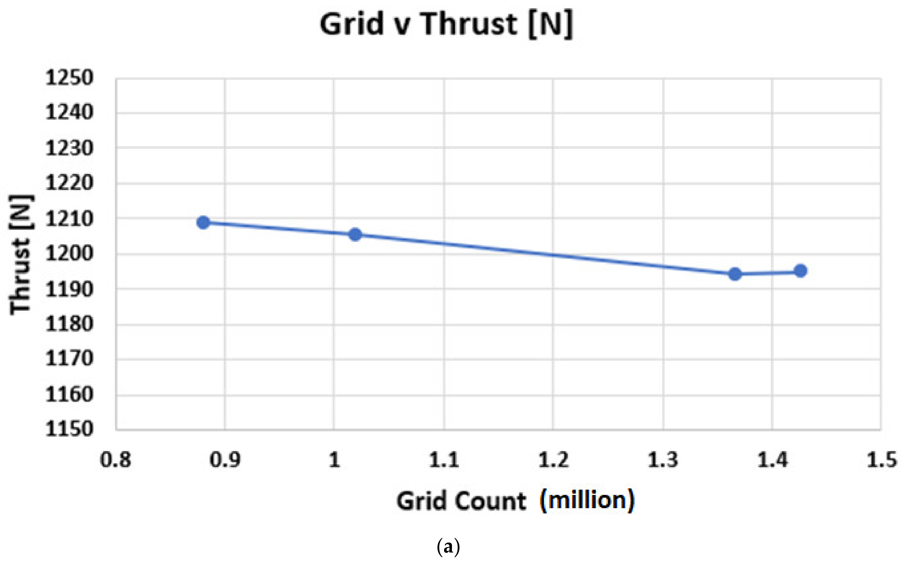
| Type | L_Up | H_Far | H_Down | Grid (×106) | Thrust (N) | Torque (Nm) | Power (kW) | CT | CP |
|---|---|---|---|---|---|---|---|---|---|
| py_BEM | 1299 | 795 | 5.90 | 0.5447 | 0.3589 | ||||
| 1X CFD domain | 5R | 5R | 25R | 0.88 | 1214 | 659 | 4.97 | 0.5091 | 0.2979 |
| 2X CFD domain | 10R | 10R | 30R | 1.10 | 1207 | 650 | 4.90 | 0.5062 | 0.2936 |
| 3X CFD domain | 15R | 15R | 40R | 1.22 | 1205 | 649 | 4.89 | 0.5053 | 0.2932 |
| 4X CFD domain | 20R | 15R | 60R | 1.46 | 1205 | 649 | 4.89 | 0.5053 | 0.2931 |
Publisher’s Note: MDPI stays neutral with regard to jurisdictional claims in published maps and institutional affiliations. |
© 2022 by the authors. Licensee MDPI, Basel, Switzerland. This article is an open access article distributed under the terms and conditions of the Creative Commons Attribution (CC BY) license (https://creativecommons.org/licenses/by/4.0/).
Share and Cite
Siddappaji, K.; Turner, M. Improved Prediction of Aerodynamic Loss Propagation as Entropy Rise in Wind Turbines Using Multifidelity Analysis. Energies 2022, 15, 3935. https://doi.org/10.3390/en15113935
Siddappaji K, Turner M. Improved Prediction of Aerodynamic Loss Propagation as Entropy Rise in Wind Turbines Using Multifidelity Analysis. Energies. 2022; 15(11):3935. https://doi.org/10.3390/en15113935
Chicago/Turabian StyleSiddappaji, Kiran, and Mark Turner. 2022. "Improved Prediction of Aerodynamic Loss Propagation as Entropy Rise in Wind Turbines Using Multifidelity Analysis" Energies 15, no. 11: 3935. https://doi.org/10.3390/en15113935
APA StyleSiddappaji, K., & Turner, M. (2022). Improved Prediction of Aerodynamic Loss Propagation as Entropy Rise in Wind Turbines Using Multifidelity Analysis. Energies, 15(11), 3935. https://doi.org/10.3390/en15113935