
CFD Modeling of Thermoacoustic Energy Conversion: A Review


Abstract
1. Introduction
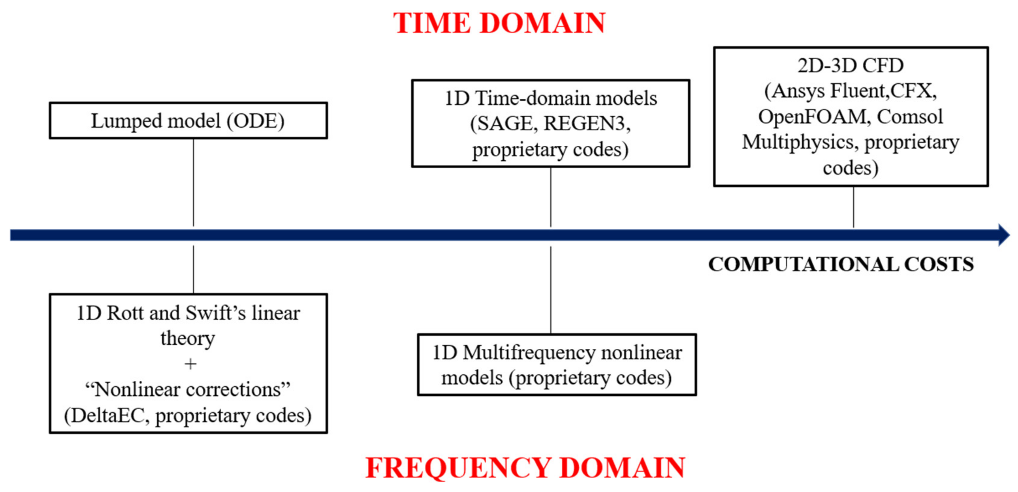
2. Thermoacoustic (TA) Modeling Approaches
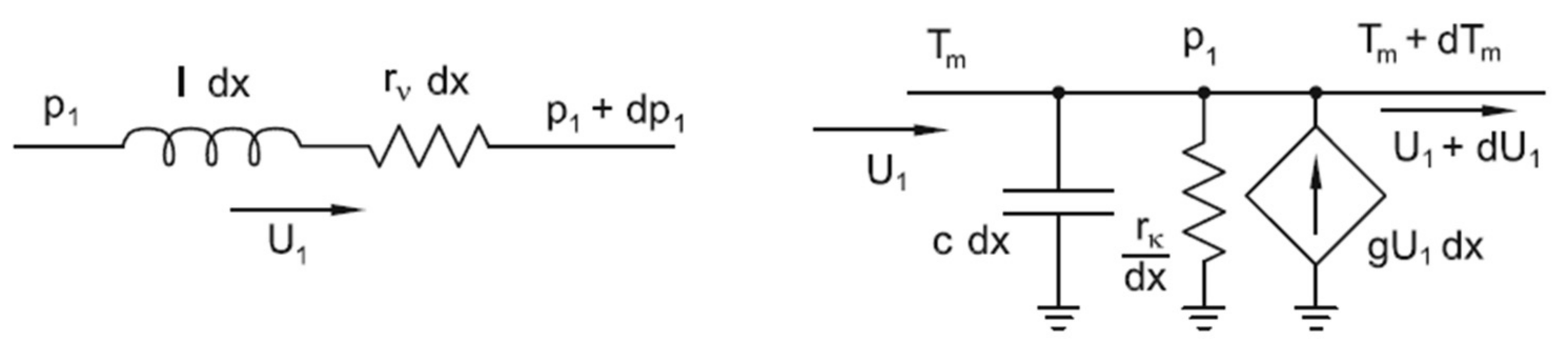
2.1. Linear Thermoacoustic Theory (LTT)
2.2. Two-Dimensional Model in Frequency Domain
2.3. Multi-Frequency Domain Approach
2.4. Lumped and 1D Time-Domain Models
2.5. CFD-Based Approach
3. Nonlinear Phenomena in Thermoacoustics
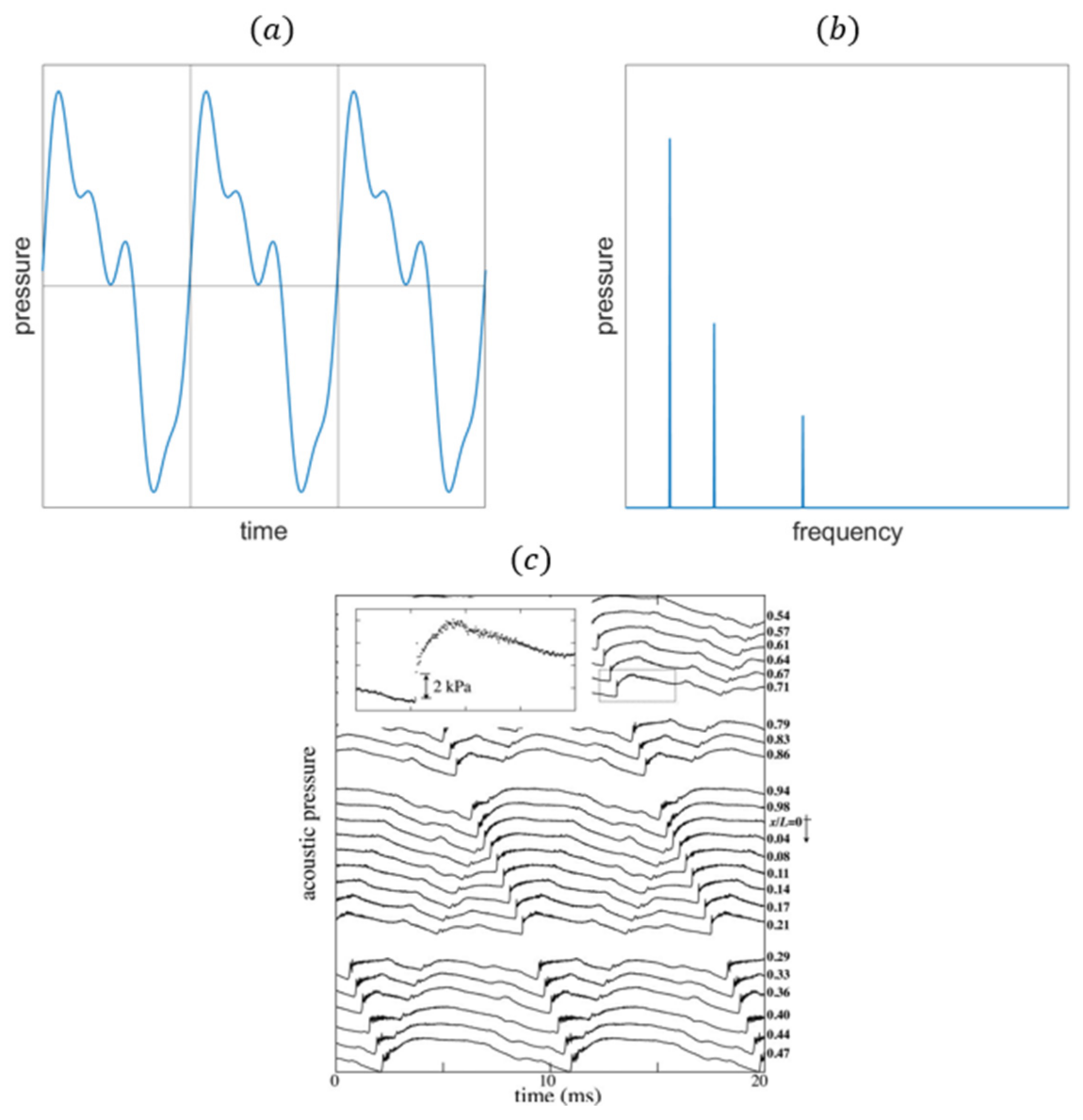
3.1. Acoustic
3.1.1. Harmonics
3.1.2. Shock Waves

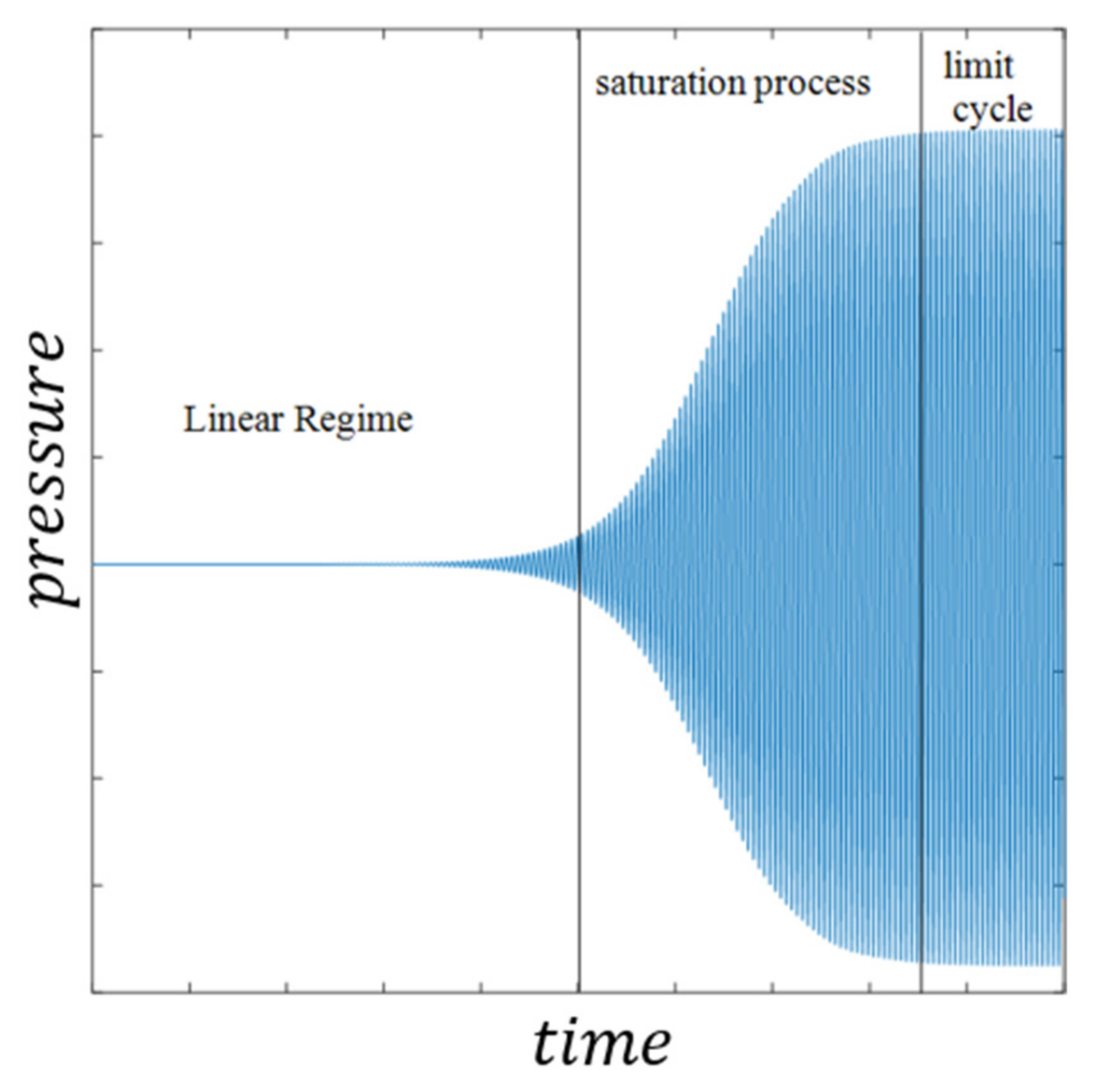
3.2. Dynamic
3.3. Hydrodynamic
3.3.1. Turbulence
3.3.2. Mass Streaming
- Gedeon streaming
- Rayleigh streaming
- Jet-driven convection
- Streaming with a regenerator or stack
3.3.3. Minor Losses
4. CFD-Based Models
4.1. Single TAC
4.2. Full Device Models
4.2.1. Microscopic Models
4.2.2. Macroscopic Models
4.2.3. General Numerical Aspects
5. Conclusions and Future Outlook
- While a traveling-wave thermoacoustic engine works at a low operating frequency and steady-state correlation for porous media can be applied, a standing-wave thermoacoustic engine, working at higher frequencies, requires specific nonlinear correlations in oscillating flows to describe the phase shift between the pressure gradient and velocity, studies on which are currently lacking in the literature.
- Heat transfer in oscillating flows between the two media in the stack of a standing-wave thermoacoustic engine is irreversible, and a local thermal non-equilibrium model is required.
- The geometries of regenerators, compared to those of stacks, are irregular and their characteristic lengths are significantly smaller and therefore difficult to be fully modeled without impacting the computational costs.
Author Contributions
Funding
Conflicts of Interest
References
- JWSB Rayleigh. The Theory of Sound; Macmillan and Co., Ltd.: New York, NY, USA, 1896. [Google Scholar]
- Abubakar, Z.; Mokheimer, E.M.A.; Kamal, M.M. A Review on Combustion Instabilities in Energy Generating Devices Utilizing Oxyfuel Combustion. Int. J. Energy Res. 2021, 45, 17461–17479. [Google Scholar] [CrossRef]
- Juniper, M.P.; Sujith, R.I. Sensitivity and Nonlinearity of Thermoacoustic Oscillations. Annu. Rev. Fluid Mech. 2018, 50, 661–689. [Google Scholar] [CrossRef]
- Timmer, M.A.G.; De Blok, K.; Van Der Meer, T.H. Review on the Conversion of Thermoacoustic Power into Electricity. Cit. J. Acoust. Soc. Am. 2018, 143, 841. [Google Scholar] [CrossRef] [PubMed]
- Wang, K.; Sanders, S.R.; Dubey, S.; Choo, F.H.; Duan, F. Stirling Cycle Engines for Recovering Low and Moderate Temperature Heat: A Review. Renew. Sustain. Energy Rev. 2016, 62, 89–108. [Google Scholar] [CrossRef]
- Jin, T.; Huang, J.; Feng, Y.; Yang, R.; Tang, K.; Radebaugh, R. Thermoacoustic Prime Movers and Refrigerators: Thermally Powered Engines without Moving Components. Energy 2015, 93, 828–853. [Google Scholar] [CrossRef]
- Steiner, T.W.; Hoy, M.; Antonelli, K.B.; Malekian, M.; Archibald, G.D.S.; Kanemaru, T.; Aitchison, W.; de Chardon, B.; Gottfried, K.T.; Elferink, M.; et al. High-Efficiency Natural Gas Fired 1 KWe Thermoacoustic Engine. Appl. Therm. Eng. 2021, 199, 117548. [Google Scholar] [CrossRef]
- Swift, G.W. Thermoacoustics: A Unifying Perspective for Some Engines and Refrigerators, 2nd ed.; Springer: Berlin/Heidelberg, Germany, 2017; ISBN 9783319669328. [Google Scholar]
- Avent, A.W.; Bowen, C.R. Principles of Thermoacoustic Energy Harvesting. Eur. Phys. J. Spec. Top. 2015, 224, 2967–2992. [Google Scholar] [CrossRef]
- Pillai, M.A.; Deenadayalan, E. A Review of Acoustic Energy Harvesting. Int. J. Precis. Eng. Manuf. 2014, 15, 949–965. [Google Scholar] [CrossRef]
- Chen, G.; Tang, L.; Mace, B.; Yu, Z. Multi-Physics Coupling in Thermoacoustic Devices: A Review. Renew. Sustain. Energy Rev. 2021, 146, 111170. [Google Scholar] [CrossRef]
- Iniesta, C.; Olazagoitia, J.L.; Vinolas, J.; Aranceta, J. Review of Travelling-Wave Thermoacoustic Electric-Generator Technology. Proc. Inst. Mech. Eng. Part A J. Power Energy 2018, 232, 940–957. [Google Scholar] [CrossRef]
- Zolpakar, N.A.; Mohd-Ghazali, N.; Hassan El-Fawal, M. Performance Analysis of the Standing Wave Thermoacoustic Refrigerator: A Review. Renew. Sustain. Energy Rev. 2016, 54, 626–634. [Google Scholar] [CrossRef]
- Clark, J.P.; Ward, W.C.; Swift, G.W. Design Environment for Low-Amplitude Thermoacoustic Energy Conversion (DeltaEC). J. Acoust. Soc. Am. 2007, 122, 3014. [Google Scholar] [CrossRef]
- Rott, N. Thermoacoustics. Adv. Appl. Mech. 1980, 20, 135–175. [Google Scholar]
- Swift, G.W. Thermoacoustic Engines. J. Acoust. Soc. Am. 1988, 84, 1145–1180. [Google Scholar] [CrossRef]
- Chen, G.; Tang, L.; Mace, B.R. Theoretical and Experimental Investigation of the Dynamic Behaviour of a Standing-Wave Thermoacoustic Engine with Various Boundary Conditions. Int. J. Heat Mass Transf. 2018, 123, 367–381. [Google Scholar] [CrossRef]
- Chen, G.; Tang, L.; Mace, B.R. Modelling and Analysis of a Thermoacoustic-Piezoelectric Energy Harvester. Appl. Therm. Eng. 2019, 150, 532–544. [Google Scholar] [CrossRef]
- Di Meglio, A.; Di Giulio, E.; Dragonetti, R.; Massarotti, N. Analysis of Heat Capacity Ratio on Porous Media in Oscillating Flow. Int. J. Heat Mass Transf. 2021, 179, 121724. [Google Scholar] [CrossRef]
- Swift, G.W. Analysis and Performance of a Large Thermoacoustic Engine. J. Acoust. Soc. Am. 1992, 92, 1551–1563. [Google Scholar] [CrossRef]
- Guedra, M.; Penelet, G. On the Use of a Complex Frequency for the Description of Thermoacoustic Engines. Acta Acust. united with Acust. 2012, 98, 232–241. [Google Scholar] [CrossRef]
- Dan, Z.; Guan, Y. Characterizing Modal Exponential Growth Behaviors of Self-Excited Transverse and Longitudinal Thermoacoustic Instabilities. Phys. Fluids 2022, 34, 024109. [Google Scholar] [CrossRef]
- De Jong, J.A.; Wijnant, Y.H.; De Boer, A. Finite Element Simulation of a Two-Dimensional Standing Wave Thermoacoustic Engine. Proc. Meet. Acoust. 2013, 19, 030002. [Google Scholar] [CrossRef]
- Muralidhar, K.; Suzuki, K. Analysis of Flow and Heat Transfer in a Regenerator Mesh Using a Non-Darcy Thermally Non-Equilibrium Model. Int. J. Heat Mass Transf. 2001, 44, 2493–2504. [Google Scholar] [CrossRef]
- Vafai, K. Handbook of Porous Media, 2nd ed.; CRC Press: Boca Raton, FL, USA, 2005; ISBN 9780415876384. [Google Scholar]
- Gheisari, R.; Jafarian, A.; Ansari, M.R. Analytical Investigation of Compressible Oscillating Flow in a Porous Media: A Second-Order Successive Approximation Technique. Int. J. Refrig. 2012, 35, 1789–1799. [Google Scholar] [CrossRef]
- Tanaka, M.; Yamashita, I.; Chisaka, F. Flow and Heat Transfer Characteristics of the Stirling Engine Regenerator in an Oscillating Flow. JSME Int. J. 1990, 33, 283–289. [Google Scholar] [CrossRef]
- De Jong, J.A.; Wijnant, J.H.; Wilcox, D.; de Boer, A. Modeling of Thermoacoustic Systems Using the Nonlinear Frequency Domain Method. J. Acoust. Soc. Am. 2015, 138, 1241. [Google Scholar] [CrossRef]
- Yuan, H.; Karpov, S.; Prosperetti, A. A Simplified Model for Linear and Nonlinear Processes in Thermoacoustic Prime Movers. Part II. Nonlinear Oscillations. J. Acoust. Soc. Am. 1997, 102, 3497–3506. [Google Scholar] [CrossRef]
- Watanabe, M.; Prosperetti, A.; Yuan, H. A Simplified Model for Linear and Nonlinear Processes in Thermoacoustic Prime Movers. Part I. Model and Linear Theory. J. Acoust. Soc. Am. 1997, 102, 3484–3496. [Google Scholar] [CrossRef]
- Karpov, S.; Prosperetti, A. A Nonlinear Model of Thermoacoustic Devices. J. Acoust. Soc. Am. 2002, 112, 1431–1444. [Google Scholar] [CrossRef]
- Karpov, S.; Prosperetti, A. Linear Thermoacoustic Instability in the Time Domain. J. Acoust. Soc. Am. 2014, 103, 3309–3317. [Google Scholar] [CrossRef]
- Karpov, S.; Prosperetti, A. Nonlinear Saturation of the Thermoacoustic Instability. J. Acoust. Soc. Am. 2000, 24, 3130–3147. [Google Scholar] [CrossRef]
- Wang, K.; Sun, D.M.; Zhang, J.; Zou, J.; Wu, K.; Qiu, L.M.; Huang, Z.Y. Numerical Simulation on Onset Characteristics of Traveling-Wave Thermoacoustic Engines Based on a Time-Domain Network Model. Int. J. Therm. Sci. 2015, 94, 61–71. [Google Scholar] [CrossRef]
- Swift, G.W.; Ward, W.C. Simple Harmonic Analysis of Regenerators. J. Thermophys. Heat Transf. 1996, 10, 652–662. [Google Scholar] [CrossRef]
- Penelet, G.; Guedra, M.; Gusev, V.; Devaux, T. Simplified Account of Rayleigh Streaming for the Description of Nonlinear Processes Leading to Steady State Sound in Thermoacoustic Engines. Int. J. Heat Mass Transf. 2012, 55, 6042–6053. [Google Scholar] [CrossRef]
- Zare, S.; Tavakolpour-Saleh, A.R. Modeling, Construction, and Testing of a Diaphragm Thermoacoustic Stirling Engine. Energy Convers. Manag. 2021, 243, 114394. [Google Scholar] [CrossRef]
- Matveev, K.I. Unsteady Model for Standing-Wave Thermoacoustic Engines. J. Non-Equilibrium Thermodyn. 2010, 35, 85–96. [Google Scholar] [CrossRef]
- Penelet, G.; Gusev, V.; Lotton, P.; Bruneau, M. Experimental and Theoretical Study of Processes Leading to Steady-State Sound in Annular Thermoacoustic Engines. Phys. Rev. E - Stat. Nonlinear, Soft Matter Phys. 2005, 72, 1–13. [Google Scholar] [CrossRef]
- Guedra, M.; Penelet, G.; Lotton, P. Experimental and Theoretical Study of the Dynamics of Self-Sustained Oscillations in a Standing Wave Thermoacoustic Engine. J. Appl. Phys. 2014, 115, 024504. [Google Scholar] [CrossRef]
- Boroujerdi, A.A.; Ziabasharhagh, M. Investigation of a High Frequency Pulse Tube Cryocooler Driven by a Standing Wave Thermoacoustic Engine. Energy Convers. Manag. 2014, 86, 194–203. [Google Scholar] [CrossRef]
- Sun, D.; Luo, K.; Zhang, J.; Yu, Y.S.W.; Pan, H. A Novel Non-Linear One-Dimensional Unsteady Model for Thermoacoustic Engine and Its Application on a Looped Traveling-Wave Thermoacoustic Engine. Appl. Acoust. 2021, 181, 108136. [Google Scholar] [CrossRef]
- Luo, K.; Zhang, L.; Hu, J.; Luo, E.; Wu, Z.; Sun, Y.; Zhou, Y. Numerical Investigation on a Heat-Driven Free-Piston Thermoacoustic-Stirling Refrigeration System with a Unique Configuration for Recovering Low-to-Medium Grade Waste Heat. Int. J. Refrig. 2021, 130, 140–149. [Google Scholar] [CrossRef]
- Gedeon, D. Sage User’s Guide; Sage Accpac International, Inc.: Pleasanton, CA, USA, 2021. [Google Scholar]
- Li, X.; Liu, B.; Yu, G.; Dai, W.; Hu, J.; Luo, E.; Li, H. Experimental Validation and Numeric Optimization of a Resonance Tube-Coupled Duplex Stirling Cooler. Appl. Energy 2017, 207, 604–612. [Google Scholar] [CrossRef]
- Gary, J.; O’Gallagher, A.; Radebaugh, R. A Numerical Model for Regenerator Performance; Technical Report; NIST: Boulder, CO, USA, 1994. [Google Scholar]
- Li, Z.F.; Qiu, L.M.; Liu, G.J.; Wang, B.; Hu, J.-Q. Simulation and Experimental Study of Pulse Tube Cooler Driven by Thermoacoustic Engine. J. Zhejiang Univ. 2009, 43, 1458–1462. [Google Scholar]
- Marx, D.; Blanc-Benon, P. Computation of the Temperature Distortion in the Stack of a Standing-Wave Thermoacoustic Refrigerator. J. Acoust. Soc. Am. 2005, 118, 2993–2999. [Google Scholar] [CrossRef]
- Gusev, V.; Hélène, B.; Pierrick, L.; Stéphane, J.; Bruneau, M. Enhancement of the Q of a Nonlinear Acoustic Resonator by Active Suppression of Harmonics. J. Acoust. Soc. Am. 1998, 12, 177–179. [Google Scholar] [CrossRef]
- Gupta, P.; Lodato, G.; Scalo, C. Numerical Investigation and Modeling of Thermoacoustic Shock Waves. In Proceedings of the AIAA SciTech Forum-55th AIAA Aerospace Scinces Meeting, Grapevine, TX, USA, 9–13 January 2017. [Google Scholar] [CrossRef]
- Gupta, P.; Lodato, G.; Scalo, C. Spectral Energy Cascade in Thermoacoustic Shock Waves. J. Fluid Mech. 2017, 831, 358–393. [Google Scholar] [CrossRef]
- Olivier, C.; Penelet, G.; Poignand, G.; Gilbert, J.; Lotton, P. Weakly Nonlinear Propagation in Thermoacoustic Engines: A Numerical Study of Higher Harmonics Generation up to the Appearance of Shock Waves. Acta Acust. United Acust. 2015, 101, 941–949. [Google Scholar] [CrossRef]
- Biwa, T.; Takahashi, T.; Yazaki, T. Observation of Traveling Thermoacoustic Shock Waves (L). J. Acoust. Soc. Am. 2011, 130, 3558–3561. [Google Scholar] [CrossRef]
- Hantschk, C.C.; Vortmeyer, D. Numerical Simulation of Self-Excited Thermoacoustic Instabilities in a Rijke Tube. J. Sound Vib. 1999, 227, 511–522. [Google Scholar] [CrossRef]
- Chen, G.; Tang, L.; Yu, Z. Underlying Physics of Limit-Cycle, Beating and Quasi-Periodic Oscillations in Thermoacoustic Devices. J. Phys. D Appl. Phys. 2020, 53, 215502. [Google Scholar] [CrossRef]
- Delage, R.; Takayama, Y.; Hyodo, H.; Biwa, T. Observation of Thermoacoustic Chaotic Oscillations in a Looped Tube. Chaos 2019, 29, 093108. [Google Scholar] [CrossRef]
- Chen, G.; Tang, L.; Yu, Z.; Mace, B. Mode Transition in a Standing-Wave Thermoacoustic Engine: A Numerical Study. J. Sound Vib. 2021, 504, 116119. [Google Scholar] [CrossRef]
- Chen, G.; Tang, L.; Mace, B.R. Bistability and Triggering in a Thermoacoustic Engine: A Numerical Study. Int. J. Heat Mass Transf. 2020, 157, 119951. [Google Scholar] [CrossRef]
- Chen, M.; Ju, Y.L. Experimental Study of Quasi-Periodic on-off Phenomena in a Small-Scale Traveling Wave Thermoacoustic Heat Engine. Cryogenics 2017, 85, 23–29. [Google Scholar] [CrossRef]
- Yu, Z.; Jaworski, A.J.; Abduljalil, A.S. Fishbone-like Instability in a Looped-Tube Thermoacoustic Engine. J. Acoust. Soc. Am. 2010, 128, EL188–EL194. [Google Scholar] [CrossRef] [PubMed]
- Feldmann, D.; Wagner, C. Direct Numerical Simulation of Fully Developed Turbulent and Oscillatory Pipe Flows at Reτ = 1440. J. Turbul. 2012, 13, 1–28. [Google Scholar] [CrossRef]
- Hino, M.; Sawamoto, M.; Takasu, S. Experiments on Transition to Turbulence in an Oscillatory Pipe Flow. J. Fluid Mech. 1976, 75, 193–207. [Google Scholar] [CrossRef]
- Seume, J.; Friedman, G.; Simon, T.W. Fluid Mechanics Experiments in Oscillatory Flow; Technical report NASA CR-189127; NASA: Washington, DC, USA, 1992. [Google Scholar]
- Simon, T.W.; Ibrahim, M.; Kannapareddy, M.; Johnson, T.; Friedman, G. Transition of Oscillatory Flow in Tubes: An Empirical Model for Application to Stirling Engines. SAE Tech. Pap. 1992. [Google Scholar] [CrossRef]
- Mohd Saat, F.A.Z.; Jaworski, A.J. Numerical Predictions of Early Stage Turbulence in Oscillatory Flow across Parallel-Plate Heat Exchangers of a Thermoacoustic System. Appl. Sci. 2017, 7, 673. [Google Scholar] [CrossRef]
- Huang, H.; Jaworski, A. Numerical Simulation of the Effect of Plate Spacing on Heat Transfer Characteristics within a Parallel-Plate Heat Exchanger in a Standing Wave Thermoacoustic System. E3S Web Conf. 2019, 116, 00028. [Google Scholar] [CrossRef]
- Ramadan, I.; Essawey, A.H.I.; Abdel-rahman, E. Transition to Turbulence in Oscillating Flow. In Proceedings of the 24th International Congress on Sound and Vibration, London, UK, 23–27 July 2017. [Google Scholar]
- Merkli, P.; Thomann, H. Transition to Turbulence in Oscillating Pipe Flow. J. Fluid Mech. 1975, 68, 567–576. [Google Scholar] [CrossRef]
- Scalo, C.; Lele, S.K.; Hesselink, L. Linear and Nonlinear Modelling of a Theoretical Travelling-Wave Thermoacoustic Heat Engine. J. Fluid Mech. 2015, 766, 368–404. [Google Scholar] [CrossRef]
- Lin, J.; Scalo, C.; Hesselink, L. High-Fidelity Simulation of a Standing-Wave Thermoacoustic-Piezoelectric Engine. J. Fluid Mech. 2016, 808, 19–60. [Google Scholar] [CrossRef]
- Mahdaoui, M.; Bennacer, R.; Kouidri, S.; Martaj, N. Numerical Investigation of Thermoacoustic Engine Using Implicit Large Eddy Simulation. In Proceedings of the 7th European Congress on Computational Methods in Applied Sciences and Engineering, Crete Island, Greece, 5–10 June 2016; Volume 4, pp. 7609–7619. [Google Scholar] [CrossRef]
- Ali, M.M.; Martaj, N.; Laaouatni, A.; Savarese, S.; Bennacer, R.; Kouidri, S. 2D Simulation of the Oscillating Flow in the Thermoacoustic Engine Swift Backhaus. In Proceedings of the International Renewable and Sustainable Energy Conference (IRSEC), Marrakech, Morocco, 14–17 November 2016; pp. 862–865. [Google Scholar] [CrossRef]
- Ahn, K.H.; Ibrahim, M.B. Laminar/Turbulent Oscillating Flow in Circular Pipes. Int. J. Heat Fluid Flow 1992, 13, 340–346. [Google Scholar] [CrossRef]
- Chen, G.; Wang, Y.; Tang, L.; Wang, K.; Yu, Z. Large Eddy Simulation of Thermally Induced Oscillatory Flow in a Thermoacoustic Engine. Appl. Energy 2020, 276, 115458. [Google Scholar] [CrossRef]
- Jaworski, A.J.; Mao, X.; Mao, X.; Yu, Z. Entrance Effects in the Channels of the Parallel Plate Stack in Oscillatory Flow Conditions. Exp. Therm. Fluid Sci. 2009, 33, 495–502. [Google Scholar] [CrossRef]
- Lixian, G.; Dan, Z.; Sid, B. Temperature Difference and Stack Plate Spacing Effects on Thermodynamic Performances of Standing-Wave Thermoacoustic Engines Driven by Cryogenic Liquids and Waste Heat. J. Therm. Sci. 2022, 31, 1–18. [Google Scholar]
- Spalart, P.R. Detached-Eddy Simulation. Annu. Rev. Fluid Mech. 2009, 41, 181–202. [Google Scholar] [CrossRef]
- Boluriaan, S.; Morris, P.J. Acoustic Streaming: From Rayleigh to Today. Int. J. Aeroacoustics 2003, 2, 255–292. [Google Scholar] [CrossRef]
- Oosterhuis, J.P.; Bühler, S.; Wilcox, D.; Van Der Meer, T.H. Computational Fluid Dynamics Simulation of Rayleigh Streaming in a Vibrating Resonator. Proc. Meet. Acoust. 2013, 19, 030008. [Google Scholar] [CrossRef]
- Chen, G.; Krishan, G.; Yang, Y.; Tang, L.; Mace, B. Numerical Investigation of Synthetic Jets Driven by Thermoacoustic Standing Waves. Int. J. Heat Mass Transf. 2020, 146, 118859. [Google Scholar] [CrossRef]
- Shi, L.; Yu, Z.; Jaworski, A.J. Vortex Shedding Flow Patterns and Their Transitions in Oscillatory Flows Past Parallel-Plate Thermoacoustic Stacks. Exp. Therm. Fluid Sci. 2010, 34, 954–965. [Google Scholar] [CrossRef]
- Olson, J.R.; Swift, G.W. Energy Dissipation in Oscillating Flow through Straight and Coiled Pipes. J. Acoust. Soc. Am. 1996, 100, 2123–2131. [Google Scholar] [CrossRef]
- Yiyi, M.; Xiujuan, X.; Shaoqi, Y.; Qing, L. Study on Minor Losses around the Thermoacoustic Parallel Stack in the Oscillatory Flow Conditions. Phys. Procedia 2015, 67, 485–490. [Google Scholar] [CrossRef][Green Version]
- Lycklama À Nijeholt, J.A.; Tijani, M.E.H.; Spoelstra, S.; Loginov, M.S.; Kuczaj, A.K. CFD Modeling of Streaming Phenomena in a Torus-Shaped Thermoacoustic Engine. In Proceedings of the 19th International Congress on Sound and Vibration, ICSV 2012, Vilnius, Lithuania, 8–12 July 2012; Volume 3, pp. 2024–2031. [Google Scholar]
- Yu, G.Y.; Luo, E.C.; Dai, W.; Hu, J.Y. Study of Nonlinear Processes of a Large Experimental Thermoacoustic- Stirling Heat Engine by Using Computational Fluid Dynamics. J. Appl. Phys. 2007, 102, 074901. [Google Scholar] [CrossRef]
- Yang, P.; Chen, H.; Liu, Y. Numerical Investigation on Nonlinear Effect and Vortex Formation of Oscillatory Flow throughout a Short Tube in a Thermoacoustic Stirling Engine. J. Appl. Phys. 2017, 121, 214902. [Google Scholar] [CrossRef]
- Backhaus, S.; Swift, G.W. A Thermoacoustic-Stirling Heat Engine: Detailed Study. J. Acoust. Soc. Am. 2000, 107, 3148–3166. [Google Scholar] [CrossRef]
- Boluriaan, S.; Morris, P.J. Suppression of Traveling Wave Streaming Using a Jet Pump. In Proceedings of the 41st Aerospace Sciences Meeting and Exhibit, Reno, NV, USA, 6–9 January 2003. [Google Scholar]
- Oosterhuis, J.P.; Bühler, S.; van der Meer, T.H.; Wilcox, D. A Numerical Investigation on the Vortex Formation and Flow Separation of the Oscillatory Flow in Jet Pumps. J. Acoust. Soc. Am. 2015, 137, 1722–1731. [Google Scholar] [CrossRef]
- Timmer, M.A.G.; Oosterhuis, J.P.; Bühler, S.; Wilcox, D.; van der Meer, T.H. Characterization and Reduction of Flow Separation in Jet Pumps for Laminar Oscillatory Flows. J. Acoust. Soc. Am. 2016, 139, 193–203. [Google Scholar] [CrossRef]
- Oosterhuis, J.P.; Verbeek, A.A.; Bühler, S.; Wilcox, D.; van der Meer, T.H. Flow Separation and Turbulence in Jet Pumps for Thermoacoustic Applications. Flow, Turbul. Combust. 2017, 98, 311–326. [Google Scholar] [CrossRef]
- Ohmi, M.; Iguchi, M. Critical Reynolds Number in an Oscillating Pipe Flow. Bull. JSME 1982, 25, 165–172. [Google Scholar] [CrossRef]
- Rahpeima, R.; Ebrahimi, R. Numerical Investigation of the Effect of Stack Geometrical Parameters and Thermo-Physical Properties on Performance of a Standing Wave Thermoacoustic Refrigerator. Appl. Therm. Eng. 2019, 149, 1203–1214. [Google Scholar] [CrossRef]
- Mergen, S.; Yıldırım, E.; Turkoglu, H. Numerical Study on Effects of Computational Domain Length on Flow Field in Standing Wave Thermoacoustic Couple. Cryogenics 2019, 98, 139–147. [Google Scholar] [CrossRef]
- Marx, D.; Blanc-Benon, P. Numerical Calculation of the Temperature Difference between the Extremities of a Thermoacoustic Stack Plate. Cryogenics 2005, 45, 163–172. [Google Scholar] [CrossRef]
- Worlikar, A.S.; Knio, O.M.; Klein, R. Numerical Simulation of a Thermoacoustic Refrigerator. J. Comput. Phys. 1998, 144, 299–324. [Google Scholar] [CrossRef]
- Marx, D.; Blanc-Benon, P. Numerical Simulation of Stack-Heat Exchangers Coupling in a Thermoacoustic Refrigerator. AIAA J. 2004, 42, 1338–1347. [Google Scholar] [CrossRef]
- Zoontjens, L.; Howard, C.Q.; Zander, A.C.; Cazzolato, B.S. Numerical Study of Flow and Energy Fields in Thermoacoustic Couples of Non-Zero Thickness. Int. J. Therm. Sci. 2009, 48, 733–746. [Google Scholar] [CrossRef]
- El-Rahman, A.I.A.; Abdel-Rahman, E. Computational Fluid Dynamics Simulation of a Thermoacoustic Refrigerator. J. Thermophys. Heat Transf. 2014, 28, 78–86. [Google Scholar] [CrossRef]
- Namdar, A.; Kianifar, A.; Roohi, E. Numerical Investigation of Thermoacoustic Refrigerator at Weak and Large Amplitudes Considering Cooling Effect. Cryogenics 2015, 67, 36–44. [Google Scholar] [CrossRef]
- Cao, N.; Olson, J.R.; Swift, G.W.; Chen, S. Energy Flux Density in a Thermoacoustic Couple. J. Acoust. Soc. Am. 1996, 99, 3456–3464. [Google Scholar] [CrossRef]
- Ishikawa, H.; Mee, D.J. Numerical Investigations of Flow and Energy Fields near a Thermoacoustic Couple. J. Acoust. Soc. Am. 2002, 111, 831–839. [Google Scholar] [CrossRef]
- Ke, H.B.; Liu, Y.W.; He, Y.L.; Wang, Y.; Huang, J. Numerical Simulation and Parameter Optimization of Thermo-Acoustic Refrigerator Driven at Large Amplitude. Cryogenics 2010, 50, 28–35. [Google Scholar] [CrossRef]
- Tasnim, S.H.; Fraser, R.A. Computation of the Flow and Thermal Fields in a Thermoacoustic Refrigerator. Int. Commun. Heat Mass Transf. 2010, 37, 748–755. [Google Scholar] [CrossRef]
- Abd El-Rahman, A.I.; Abdelfattah, W.A.; Fouad, M.A. A 3D Investigation of Thermoacoustic Fields in a Square Stack. Int. J. Heat Mass Transf. 2017, 108, 292–300. [Google Scholar] [CrossRef]
- Worlikar, A.S.; Knio, O.M.; Klein, R. Numerical study of oscillatory flow and heat transfer in a loaded thermoacoustic stack. Int. J. Comput. Methodol. 1999, 35, 49–65. [Google Scholar] [CrossRef]
- Boroujerdi, A.A.; Ziabasharhagh, M. A Coupled Computational Model of Nonlinear Thermoacoustics of Standing Wave Heat Engines. Heat Mass Transf. Stoffuebertragung 2019, 55, 3223–3241. [Google Scholar] [CrossRef]
- Migliorino, M.T.; Scalo, C. Real Fluid Effects Thermoacoustic Engine.Pdf. J. Fluid Mech. 2019, 883, A23. [Google Scholar] [CrossRef]
- Marx, D.; Blanc-Benon, P. Numerical Simulation of the Coupling between Stack and Heat Exchangers in a Thermoacoustic Refrigerator. In Proceedings of the 9th AIAA/CEAS Aeroacoustics Conference and Exhibit, Hilton Head, CA, USA, 12–14 May 2003. [Google Scholar] [CrossRef]
- Hamilton, M.F.; Ilinskii, Y.A.; Zabolotskaya, E.A. Nonlinear Two-Dimensional Model for Thermoacoustic Engines. J. Acoust. Soc. Am. 2002, 111, 2076. [Google Scholar] [CrossRef]
- Ja’fari, M.; Jaworski, A.J.; Piccolo, A.; Simpson, K. Numerical Study of Transient Characteristics of a Standing-Wave Thermoacoustic Heat Engine. Int. J. Heat Mass Transf. 2022, 186, 122530. [Google Scholar] [CrossRef]
- Sharify, E.M.; Takahashi, S.; Hasegawa, S. Development of a CFD Model for Simulation of a Traveling-Wave Thermoacoustic Engine Using an Impedance Matching Boundary Condition. Appl. Therm. Eng. 2016, 107, 1026–1035. [Google Scholar] [CrossRef]
- Rogoziński, K.; Nowak, I.; Nowak, G. Modeling the Operation of a Thermoacoustic Engine. Energy 2017, 138, 249–256. [Google Scholar] [CrossRef]
- Nowak, I.; Rulik, S.; Wróblewski, W.; Nowak, G.; Szwedowicz, J. Analytical and Numerical Approach in the Simple Modelling of Thermoacoustic Engines. Int. J. Heat Mass Transf. 2014, 77, 369–376. [Google Scholar] [CrossRef]
- Zink, F.; Vipperman, J.S.; Schaefer, L.A. Advancing Thermoacoustics through CFD Simulation Using Fluent. ASME Int. Mech. Eng. Congr. Expo. Proc. 2009, 8, 101–110. [Google Scholar] [CrossRef]
- Zink, F.; Vipperman, J.; Schaefer, L. CFD Simulation of a Thermoacoustic Engine with Coiled Resonator. Int. Commun. Heat Mass Transf. 2010, 37, 226–229. [Google Scholar] [CrossRef]
- Zink, F.; Vipperman, J.; Schaefer, L. CFD Simulation of Thermoacoustic Cooling. Int. J. Heat Mass Transf. 2010, 53, 3940–3946. [Google Scholar] [CrossRef]
- Skaria, M.; Abdul Rasheed, K.K.; Shafi, K.A.; Kasthurirengan, S.; Behera, U. Simulation Studies on the Performance of Thermoacoustic Prime Movers and Refrigerator. Comput. Fluids 2015, 111, 127–136. [Google Scholar] [CrossRef]
- Ali, U.; Abedrabbo, S.; Janajreh, I. Numerical Simulation of Thermoacoustic Refrigerator Coupled with Thermoacoustic Engine. In Proceedings of the 15th International Conference On Heat Transfer, Fluid Mechanics and Thermodynamics (HEFAT), Virtual, 25–27 July 2021. [Google Scholar]
- Bouramdane, Z.; Bah, A.; Alaoui, M.; Martaj, N. Numerical Analysis of Thermoacoustically Driven Thermoacoustic Refrigerator with a Stack of Parallel Plates Having Corrugated Surfaces. Int. J. Air-Cond. Refrig. 2022, 30, 1–19. [Google Scholar] [CrossRef]
- Chen, G.; Li, Z.; Tang, L.; Yu, Z. Mutual Synchronization of Self-Excited Acoustic Oscillations in Coupled Thermoacoustic Oscillators. J. Phys. D. Appl. Phys. 2021, 54, 48. [Google Scholar] [CrossRef]
- Rogoziński, K.; Nowak, G. Numerical Investigation of Dual Thermoacoustic Engine. Energy Convers. Manag. 2020, 203, 112231. [Google Scholar] [CrossRef]
- Bouramdane, Z.; Hafs, H.; Bah, A.; Alaoui, M.; Martaj, N.; Savarese, S. Standing Wave Thermoacoustic Refrigerator: The Principle of Thermally Driven Cooling. In Proceedings of the 6th International Renewable and Sustainable Energy Conference (IRSEC), Rabat, Morocco, 5–8 December 2018; pp. 1–6. [Google Scholar] [CrossRef]
- Muralidharan, H.; Hariharan, N.M.; Perarasu, V.T.; Sivashanmugam, P.; Kasthurirengan, S. CFD Simulation of Thermoacoustic Heat Engine. Prog. Comput. Fluid Dyn. 2014, 14, 131–137. [Google Scholar] [CrossRef]
- Kuzuu, K.; Hasegawa, S. Numerical Investigation of Heated Gas Flow in a Thermoacoustic Device. Appl. Therm. Eng. 2017, 110, 1283–1293. [Google Scholar] [CrossRef]
- Kuzuu, K.; Hasegawa, S. Effect of Non-Linear Flow Behavior on Heat Transfer in a Thermoacoustic Engine Core. Int. J. Heat Mass Transf. 2017, 108, 1591–1601. [Google Scholar] [CrossRef]
- Chen, G.; Wang, Y.; Tang, L.; Wang, K.; Mace, B.R. Large Eddy simulation of self-excited acoustic oscillations in a thermoacoustic engine. In Proceedings of the International Conference on Applied Energy, Västerås, Sweden, 12–15 August 2019; pp. 1–5. [Google Scholar]
- Gupta, S.K.; Ghosh, P.; Nandi, T.K. Theoretical and CFD Investigations on a 200 Hz Thermoacoustic Heat Engine Using Pin Array Stack for Operations in a Pulse Tube Cryocooler. IOP Conf. Ser. Mater. Sci. Eng. 2019, 502, 012025. [Google Scholar] [CrossRef]
- Zhang, Y.; Shi, X.; Li, Y.; Zhang, Y.; Liu, Y. Characteristics of Thermoacoustic Conversion and Coupling Effect at Different Temperature Gradients. Energy 2020, 197, 117228. [Google Scholar] [CrossRef]
- Harikumar, G.; Shen, L.; Wang, K.; Dubey, S.; Duan, F. Transfer Transient Thermofluid Simulation of a Hybrid Thermoacoustic System. Int. J. Heat Mass Transf. 2022, 183, 122181. [Google Scholar] [CrossRef]
- Luo, J.; Zhou, Q.; Jin, T. Numerical Simulation of Nonlinear Phenomena in a Standing-Wave Thermoacoustic Engine with Gas-Liquid Coupling Oscillation. Appl. Therm. Eng. 2022, 207, 118131. [Google Scholar] [CrossRef]
- Tisovsky, T.; Vit, T. Design of Numerical Model for Thermoacoustic Devices Using OpenFOAM. AIP Conf. Proc. 2017, 1889, 020043. [Google Scholar] [CrossRef]
- Chen, G.; Hao, H.; Deng, A. Linear and Nonlinear Modeling of Self-Excited Acoustic Oscillations in a T-Shaped Thermoacoustic Engine. AIP Adv. 2021, 11, 085120. [Google Scholar] [CrossRef]
- Whitaker, S. Flow in Porous Media I: A Theoretical Derivation of Darcy’s Law. Transp. Porous Media 1986, 1, 3–25. [Google Scholar] [CrossRef]
- Whitaker, S. The Forchheimer Equation: A Theoretical Development. Transp. Porous Media 1996, 25, 27–61. [Google Scholar] [CrossRef]
- Pati, S.; Borah, A.; Boruah, M.P.; Randive, P.R. Critical Review on Local Thermal Equilibrium and Local Thermal Non-Equilibrium Approaches for the Analysis of Forced Convective Flow through Porous Media. Int. Commun. Heat Mass Transf. 2022, 132, 105889. [Google Scholar] [CrossRef]
- Miled, O.; Dhahri, H.; Mhimid, A. Numerical Investigation of Porous Stack for a Solar-Powered Thermoacoustic Refrigerator. Adv. Mech. Eng. 2020, 12, 1–14. [Google Scholar] [CrossRef]
- Yu, G.; Dai, W.; Luo, E. CFD Simulation of a 300 Hz Thermoacoustic Standing Wave Engine. Cryogenics 2010, 50, 615–622. [Google Scholar] [CrossRef]
- Liu, L.; Yang, P.; Liu, Y. Comprehensive Performance Improvement of Standing Wave Thermoacoustic Engine with Converging Stack: Thermodynamic Analysis and Optimization. Appl. Therm. Eng. 2019, 160, 114096. [Google Scholar] [CrossRef]
- ESI-CFD-Inc. CFD-ACE+ V2009.4. In User Manual; ESI Group: Hunstville, AL, USA, 2009. [Google Scholar]
- Tew, R.; Simon, T.; Gedeon, D.; Ibrahim, M.; Rong, W. An Initial Non-Equilibrium Porous-Media Model for CFD Simulation of Stirling Regenerators. In Proceedings of the 4th International Energy Conversion Engineering Conference and Exhibit, San Diego, CA, USA, 26–29 June 2006; Volume 1, pp. 65–77. [Google Scholar] [CrossRef]
- Lycklama à Nijeholt, J.A.; Tijani, M.E.H.; Spoelstra, S. Simulation of a Traveling-Wave Thermoacoustic Engine Using Computational Fluid Dynamics. J. Acoust. Soc. Am. 2005, 118, 2265–2270. [Google Scholar] [CrossRef]
- Liu, L.; Liu, Y.; Duan, F. Effect of the Characteristic Time on the System Performance of a Three-Stage Looped Traveling-Wave Thermoacoustic Engine. Energy Convers. Manag. 2020, 224, 113367. [Google Scholar] [CrossRef]
- Antao, D.S.; Farouk, B. Experimental and Numerical Investigations of an Orifice Type Cryogenic Pulse Tube Refrigerator. Appl. Therm. Eng. 2013, 50, 112–123. [Google Scholar] [CrossRef]
- Antao, D.S.; Farouk, B. Computational Fluid Dynamics Simulations of an Orifice Type Pulse Tube Refrigerator: Effects of Operating Frequency. Cryogenics 2011, 51, 192–201. [Google Scholar] [CrossRef]
- Antao, D.S.; Farouk, B. Numerical Simulations of Transport Processes in a Pulse Tube Cryocooler: Effects of Taper Angle. Int. J. Heat Mass Transf. 2011, 54, 4611–4620. [Google Scholar] [CrossRef]
- Ilori, O.M.; Jaworski, A.J.; Mao, X.; Ismail, O.S. Effects of Edge Shapes on Thermal-Fluid Processes in Oscillatory Flows. Therm. Sci. Eng. Prog. 2021, 25, 101004. [Google Scholar] [CrossRef]
- Ilori, O.M.; Jaworski, A.J.; Mao, X. Experimental and Numerical Investigations of Thermal Characteristics of Heat Exchangers in Oscillatory Flow. Appl. Therm. Eng. 2018, 144, 910–925. [Google Scholar] [CrossRef]
- Piccolo, A. Numerical Computation for Parallel Plate Thermoacoustic Heat Exchangers in Standing Wave Oscillatory Flow. Int. J. Heat Mass Transf. 2011, 54, 4518–4530. [Google Scholar] [CrossRef]
- Piccolo, A.; Pistone, G. Estimation of Heat Transfer Coefficients in Oscillating Flows: The Thermoacoustic Case. Int. J. Heat Mass Transf. 2006, 49, 1631–1642. [Google Scholar] [CrossRef]


| N° | Model | Typical Computational Domain at the Microscopic Scale of the TAC | Refs. |
|---|---|---|---|
| I | SWTAR |  | [96] [104] |
| II | SWTAR |  | [101] |
| III | SWTAR |  | [106] |
| IV | SWTAR |  | [48] [95] [102] |
| V | SWTAR |  | [103] |
| VI | SWTAR |  | [97] [93] |
| VII | SWTAR with square stack (3D) |  | [105] |
| VIII | SWTAR (SWTAE) |  | [100] [111] |
| IX | SWTAE |  | [108] [110] |
| X | SWTAE |  | [107] |
| XI | SWTAE |  | [112] |
| Refs. | Fluid | Solid | Dr (%) | Oscillating BC | Fluid–Solid Interface BC | Software | ||||
|---|---|---|---|---|---|---|---|---|---|---|
| [96] | Helium | Steel + fiberglass | 0.85 | - | 2.35 ÷ 3 | 0.28 ÷ 2 | 1/400 | Vorticity | Coupled | Proprietary |
| [101] | - | - | 1 | 0.83 ÷ 3.3 | 0.23–0.63 | 1.4 ÷ 7 | 0.024 | Velocity | Isothermal | Proprietary |
| [106] | Helium | Steel + fiberglass | 0.66 | 3.5 | 2.35 | 1.5–2.5 | 0.0195 | Velocity | Coupled | Proprietary |
| [102] | Air | - | 1 | 0.33–3.33 | 0.785 | 1.7–8.5 | 0.0023–0.05 | Pressure/velocity and temperature | Isothermal | PHOENICS |
| [95] | Air | Mylar | 1 | 1.9 | 1.5 ÷ 3.25 | 0.7 ÷ 11.2 | 0.0088 | Pressure | 1D solid energy equation | Proprietary |
| [48] | Air | - | 1 | 2.5 | 2.13 | 0.7 ÷ 11.2 | 1/40 | Pressure | Isothermal | Proprietary |
| [103] | Air, Argon | Theoretical solid | 0.57 ÷ 0.83 | 1.4–2.4 | 0.15 ÷ 0.7 | ≤16 | 0.038 ÷ 0.007 | Velocity | Coupled | Proprietary |
| [97] | Air | Mylar | 1 | 0.69 ÷ 2.7 | 2.13 ÷ 2.7 | 0.8 ÷ 16.8 | 1/40–1/20 | Pressure | Isothermal or 1D solid energy equation | Proprietary |
| [93] | Helium | Kapton, steel, glass, copper | 0.88 ÷ 0.97 | 0.63 ÷ 3.3 | 2.35 | 0.05 ÷ 1.7 | 0.009 ÷ 0.068 | Pressure/velocity and temperature | Coupled | Comsol Multiphysics |
| [105] | Helium | Cordierite | 0.787 | - | 0.51 | 1.7–8.5 | - | Velocity | Coupled | Ansys Fluent |
| [100] | Air | - | 0.8 | 2.5 | 2.41 | 1 | 0.04 | Pressure | Coupled | OpenFOAM |
| [104] | Air | Glass | 0.87 | 2.6 | 0.785 | 0.7 | 0.014 | Pressure/velocity and temperature | Coupled | STAR-CD |
| [108] | CO2 | - | 0.5 | engine | Proprietary | |||||
| [107] | Helium | Stainless steel | - | engine | Coupled | Proprietary | ||||
| [112] | Air | - | 0.75 | engine | Proprietary | |||||
| [110] | Air | - | 1 | engine | Proprietary | |||||
| [97] | Air | - | 0.8 | engine | °C | OpenFOAM | ||||
| N° | Model | Typical Computational Domain at the Microscopic Scale | Refs. |
|---|---|---|---|
| I |  | [58] [115] [116] [124] [129] | |
| II |  | [117] [118] [123] | |
| III | (2D axysymmetric) |  | [70] |
| IV | Dual SWTAE |  | [118] [121] |
| V | Dual SWTAE with piston |  | [122] |
| VI | 3D SWTAE, with parallel-plate stack |  | [74] [76] [127] |
| VII | 3D SWTA, with longitudinal pin-array stack |  | [128] |
| VIII |  | [125] [126] | |
| IX | Looped tube + resonator |  | [130] |
| X | SWTAR |  | [132] |
| XI | SWTAE |  | [133] |
| Refs. | Fluid | Fluid–Solid Interface BC | Frequency [Hz] | Turbulence | Pressure Amp.(or ΔT) | Software | |||||
|---|---|---|---|---|---|---|---|---|---|---|---|
| [115] | Air | - | - | 5125 Pa | Ansys Fluent | ||||||
| [116] | Air | 614–629 | 8584–7625 Pa | Ansys Fluent | |||||||
| [124] | Air-N2-Ar | 0.375 | 217–307 | - | Ansys Fluent | ||||||
| [129] | Air | - | ILES | Pa | Comsol-Multip. | ||||||
| [58] | Air | 0.5 | Pa | Ansys Fluent | |||||||
| [117] | [115] I stack | Ansys Fluent | |||||||||
| [118] | He, Ar, N2 | - | - | - | - | 25–125 | Pa | Ansys Fluent | |||
| [123] | 0.5 | 0.25 mm | as [115,117] | 600 | - | Comsol-Multip. | |||||
| [70] | Air | 0.3–0.6 | 0.3–0.65 mm | 60 mm | 37.5 mm | 0.510 m | 382–391 | Laminar | (unloaded)(loaded) | Proprietary | |
| [121] | Air | 0.5 | 0.1 m | 30 mm | variable | 230–420 | Pa | Ansys Fluent | |||
| [122] | - | 0.5 | 30 mm | 10 mm | 140–350 | - | Ansys Fluent | ||||
| [72,127] | Air | 0.5 | 0.1 m | 30 mm | LES | Ansys Fluent | |||||
| [128] | He | 0.91 | 0.175 mm | 0.1 m | 0.1 m | 1.2 m | 200 | 420,000 Pa | Ansys Fluent | ||
| [125,126] | Air | 0.5 | 3 mm | 1 m | 90 mm | 4.59 m | Laminar | LS-FLOW | |||
| [130] | Air | 0.625 | 0.25 | 0.55 m | 100 mm | 1.6 m | 45, 120 | , input | Ansys Fluent | ||
| [132] | Air | 1 | - | 20 mm | 85 mm | 861 mm | Thermal baffles with prescribed heat flux | 500 | - | OpenFOAM | |
| N° | Model | Typical Computational Domain at the Macroscopic Scale | Refs. |
|---|---|---|---|
| I | Theoretical TWTAE (3D) |  | [69] [85] [86] [142] |
| II | Looped tube + resonator TWTAE |  | [72] [84] |
| III | 1 of the 3 stages of a TWTAE (unrolled) (2D axysymmetric) |  | [143] |
| IV | TAOPTR (2D axysymmetric) |  | [144] [145] [146] |
| V | SWTAE |  | [131] [138] [139] |
| VI | SWTAR |  | [137] |
| Refs. | Fluid | Stack/Regenerator | HX | Frequency [Hz] | Turbulence | Pressure Amp. (or Tcooling/ΔT) | Software | ||
|---|---|---|---|---|---|---|---|---|---|
| Momentum | Energy | Momentum | Energy | ||||||
| [142] | Air | Darcy–Forchheimer (PF) | LTNE (1 equation) | Darcy–Forchheimer (PF) | LTNE (1 equation) | Laminar | No steady state | Ansys CFX | |
| [85] | Air | Darcy–Forchheimer (SF) | LTE | Darcy–Forchheimer (SF) | LTE , heat source for HHX | Ansys Fluent | |||
| [69] | Air | Darcy–Forchheimer (PF) | LTNE (1 equation) | Darcy–Forchheimer (PF) | LTNE (1 equation) | ≈60 | Laminar | 10,000 Pa | Proprietary |
| [72] | - | Darcy–Forchheimer (SF) | LTE | Darcy–Forchheimer (SF) | LTE Heat source for HHX | 22 | ILES | >10,000 Pa | Comsol Mult. |
| [84] | He | Darcy–Forchheimer (SF) | LTNE (1 equation) | Darcy–Forchheimer (SF) | LTNE (1 equation) | 114 | - | Ansys Fluent | |
| [143] | He | Darcy–Forchheimer (SF) | LTE | Darcy–Forchheimer (SF) | LTE | 76 | 550,000 Pa | Ansys Fluent | |
| [144] [145] [146] | He | Darcy–Forchheimer (SF) | LNTE (2 equations) | Darcy–Forchheimer (SF) | LNTE (2 equations) | 55–65 | - | CFD-ACE+ | |
| [138] | Air | Darcy–Forchheimer (SF) | LTE | Not considered | Not considered | - | - | Lattice-Boltzmann code | |
| [139] | He | Microscopic | Microscopic, no solid | Darcy–Forchheimer (SF) | LTE | - | 60,000 Pa | Ansys Fluent | |
| [137] | He | Microscopic | Microscopic CHT | Darcy–Forchheimer (SF) | LTE | 300 | LES | 250,000 Pa | Ansys Fluent |
Publisher’s Note: MDPI stays neutral with regard to jurisdictional claims in published maps and institutional affiliations. |
© 2022 by the authors. Licensee MDPI, Basel, Switzerland. This article is an open access article distributed under the terms and conditions of the Creative Commons Attribution (CC BY) license (https://creativecommons.org/licenses/by/4.0/).
Share and Cite
Di Meglio, A.; Massarotti, N. CFD Modeling of Thermoacoustic Energy Conversion: A Review. Energies 2022, 15, 3806. https://doi.org/10.3390/en15103806
Di Meglio A, Massarotti N. CFD Modeling of Thermoacoustic Energy Conversion: A Review. Energies. 2022; 15(10):3806. https://doi.org/10.3390/en15103806
Chicago/Turabian StyleDi Meglio, Armando, and Nicola Massarotti. 2022. "CFD Modeling of Thermoacoustic Energy Conversion: A Review" Energies 15, no. 10: 3806. https://doi.org/10.3390/en15103806
APA StyleDi Meglio, A., & Massarotti, N. (2022). CFD Modeling of Thermoacoustic Energy Conversion: A Review. Energies, 15(10), 3806. https://doi.org/10.3390/en15103806