
The Impact of the Income Gap on Carbon Emissions: Evidence from China


Abstract
1. Introduction
2. Literature Review and Research Hypothesis
2.1. Literature Review
- (1)
- The widening income gap increases carbon emissions. In this regard, scholars have studied three main aspects. Firstly, the widening income gap makes the distribution of political power more favorable to high-income groups. Although the wealth accumulation of high-income groups is generally based on the destruction of the environment, low-income groups bear higher ecological costs (Boyce, 1994) [12]. Marsiliani and Renström (2000) [13] studied the relationship between the income gap and carbon dioxide emissions in OECD countries with cross-sectional and time-series data. They concluded that the income gap is positively associated with carbon emissions. Secondly, per capita carbon consumption varies significantly between households with different incomes. Direct and indirect carbon consumption of high-income households is much higher than that of low-income families (Golley and Meng, 2012) [14]. Marsiliani and Renström (2018) [15] believed that the income gap can affect carbon emissions through the consumption possibility curve. More consumption of non-low carbon commodities by low-income groups quickly leads to the weakening of environmental policies. Thirdly, the “middle man voting” theory suggests that, ultimately, the middle group in society determines the quality of the environment (Kempf, 2005) [16]. High-income groups have higher environmental requirements, whereas low-income groups lack the power to speak. The ecological quality of a society depends on the preferences of the median voter when the income gap widens. Overall, the income gap may affect carbon emissions by affecting urbanization and residents’ consumption structure (Sun, 2016) [17]. Widening income gaps can increase carbon emissions, whereas narrowing income gaps can improve environmental quality (Padilla and Serrano, 2006) [18].
- (2)
- Widening income gaps can reduce environmental pollution caused by carbon emissions. Heerink, Mulatu and Bulte (2001) [19] found a negative relationship between the income gap and carbon emissions. They used statistics data from Sweden and Italy. Ghalwash (2008) [20] as well as Castellucci and D’Amato (2009) [21] obtained the same findings that suggest that a widening income gap can reduce carbon emissions. Using statistics data from China, Lu and Gao (2005) [22] found that the widening income gap may inhibit environmental pollution when economic development reaches a particular stage.
- (3)
- There is no single linear relationship between the income gap and carbon emissions. Soytas, Sari and Ewing (2007) [23] found no causal relationship between economic development and carbon emissions using US statistics data from 1960 to 2004. The relationship between income inequality and the environment is heterogeneous (Ravallion, Heil and Jalan, 2000) [24]. Han et al. (2018) [25] found that the income gap across economies is positively related to carbon emissions. However, the relationship between them is not uncertain for regions with different incomes. Jorgenson et al. (2016) [26] used a two-way fixed-effects model to study the relationship between carbon emissions and the income gap. It was found that there is a non-linear relationship between them, and there is heterogeneity in different countries. Zhanhua (2016) [27] found that, in regions with high per capita income, narrowing the income gap can curb carbon emissions. Ma Xiaowei et al. (2019) [28] found a non-linear positive relationship between income and carbon emissions from residents’ consumption in China. For provinces in different income groups, when the income group changes, carbon emission inequality shows different trends. Zhang Yunhui and Hao Shiyu (2022) [29] used Chinese provincial panel data from 2005 to 2017 to conduct an empirical test. The effect and mechanism of income disparity and economic agglomeration on carbon emissions were investigated, and the results show that there is a significant “U” shaped relationship between the income gap and carbon emissions in China.
2.2. Influence Mechanism and Research Hypothesis of the Income Gap on Regional Carbon Emission Intensity
- (1)
- Influence mechanism
- (2)
- Research hypothesis
3. Measurement of the Income Gap and Carbon Emissions
3.1. Calculating the Income Gap between Provinces in China
- (1)
- Estimation method of the Gini coefficient of provincial resident income
- (2)
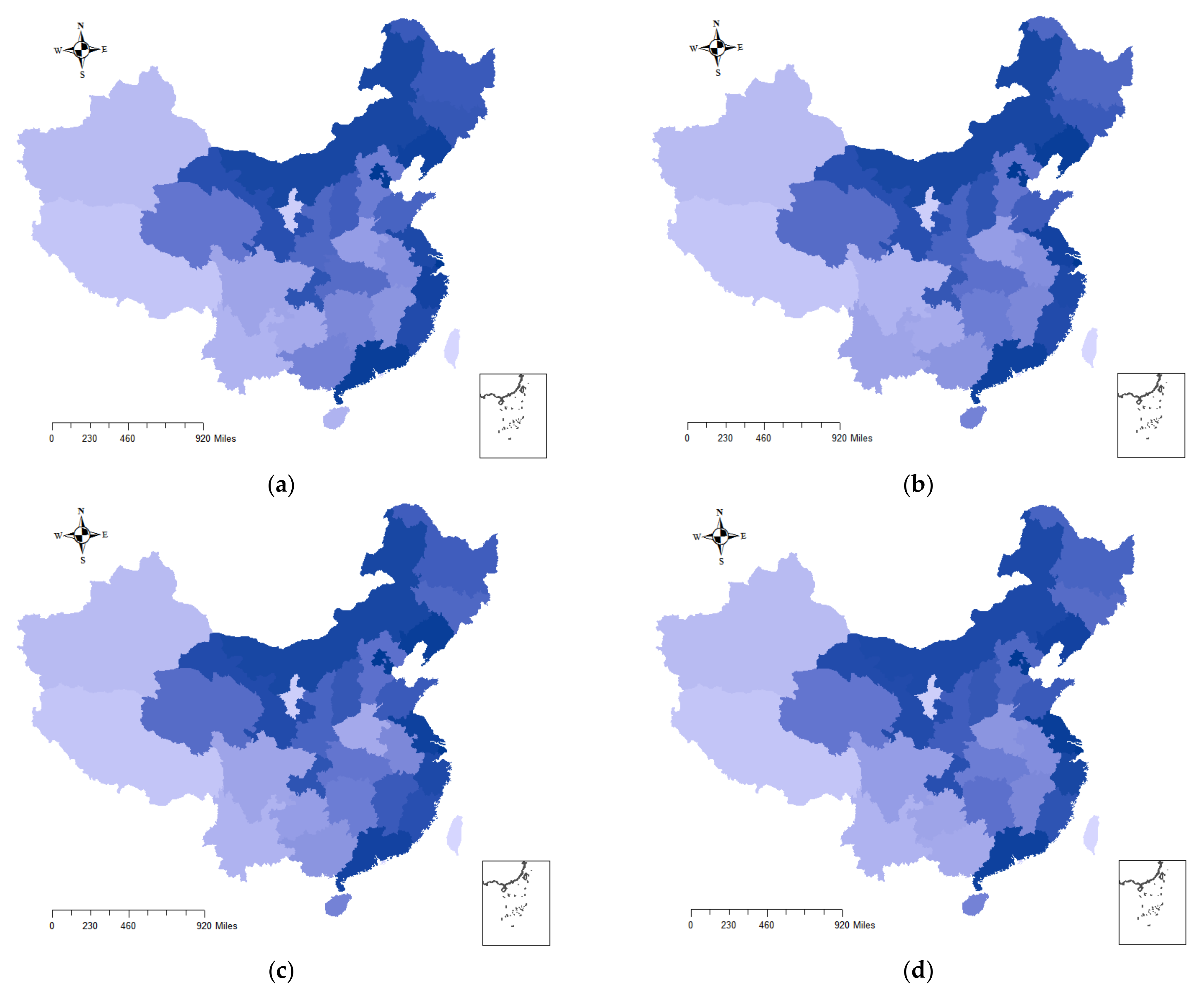
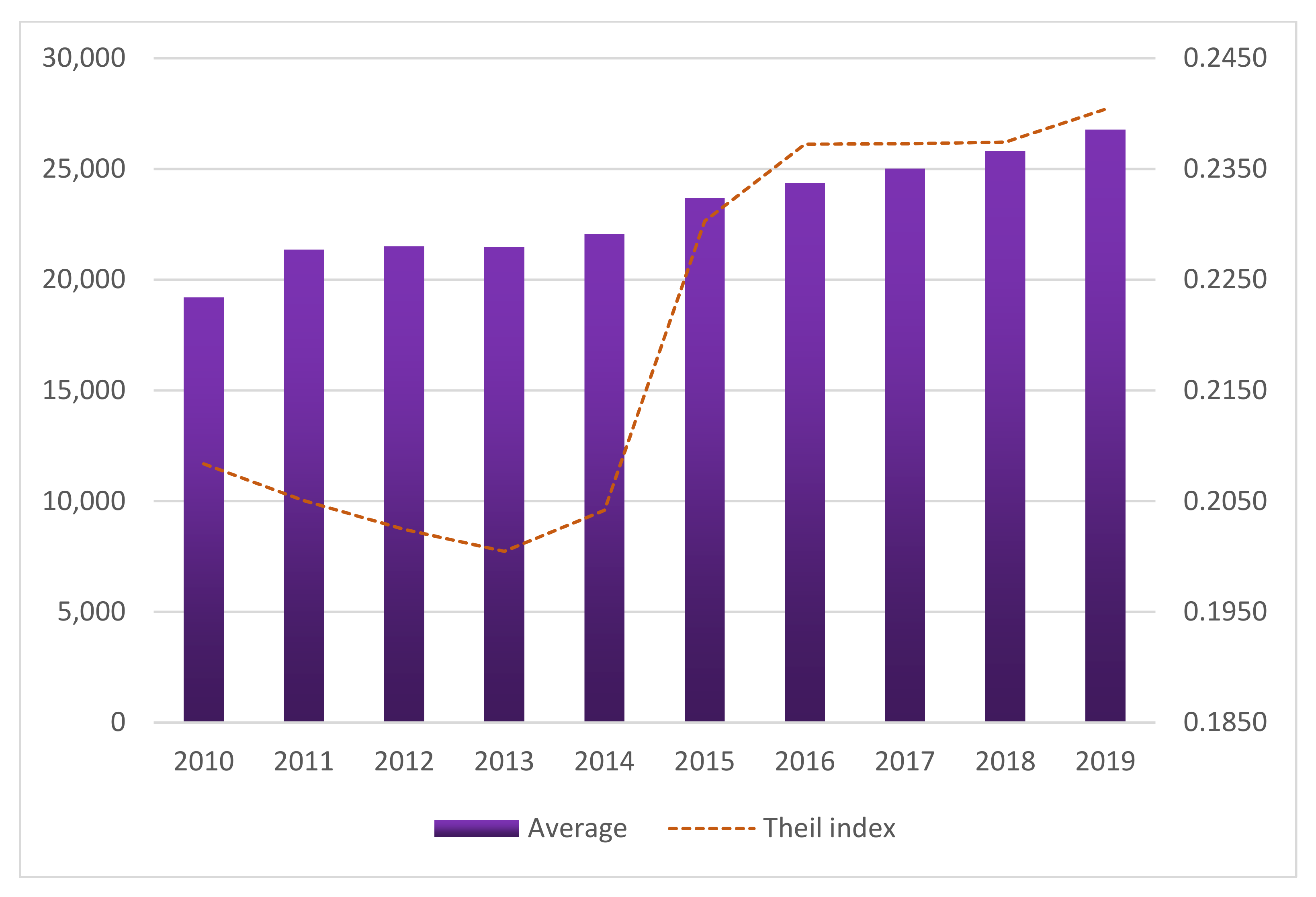
- Analysis of the results of the income gap between provincial residents
3.2. Estimating Provincial Carbon Emissions in China
- (1)
- Methodology for estimating provincial carbon emissions in China
- (2)
- Differences in carbon emissions
- (3)
- Moran index of carbon emissions
4. Research Design and Empirical Results
4.1. Model Setting and Variable Description
- (1)
- Explained variable: carbon emission intensity ()
- (2)
- Explanatory variable: income gap ().
- (3)
- Threshold variable: per capita disposable income of residents ().
- (4)
- Control variables. The control variables selected in this paper are as follows:
4.2. Empirical Results
- (1)
- Due to the limitation of green innovation technology and the neglect of the environment in a rush to economic development, some people have obtained high incomes through the destruction of the environment. The income gap widens and generates a higher pollution effect, which causes an increase in carbon emission intensity.
- (2)
- The widening income gap leads to consumption upgrades, which leads to an increase in carbon emission intensity. Under the comparison effect, the widening of intra-regional income inequality significantly increases the consumption of a region. In addition, it makes the proportion of enjoyment-oriented consumption increase significantly. Specifically, the income gap can change market supply and demand by affecting commodity markets and factor markets, affecting carbon emission intensity. On the one hand, this is also related to the ratio of access to higher education by regional residents. In low-income regions, residents have low rates of access to higher education. As a result, there is less emphasis on clean energy and products, and they prefer to consume inexpensive but carbon-intensive commodities. On the other hand, consumption upgrades have increased households’ fuel demand for travel, heating and cooking, increasing households’ direct carbon emissions. However, in the low-income stage, reducing carbon emission intensity cannot be achieved solely by narrowing the income gap because it inhibits economic development. Firstly, with the per capita income of residents gradually increasing, the impact of the widening income gap on carbon emission intensity decreases. When per capita income enters a high-income stage, the digital economy develops rapidly. The use of the Internet affects the productivity of factors such as capital, labor and information. Changes in factor productivity, in turn, affect the demand for capital and labor. The widening of the income gap at this stage is mainly due to the distributional role of the tertiary sector on income. Although the income gap has widened further with economic development, carbon emission intensity has been suppressed. Secondly, more people have entered the middle class, and the consumption structure of Chinese residents has changed. The pursuit of green and healthy food by middle-income and high-income groups has effectively reduced household carbon emissions. Higher demands on travel, heating and cooking and higher education rates have also increased residents’ attention to the environment. In the high-income stage, the widening income gap inhibits the growth of carbon emission intensity. By 2019, the per capita disposable income of most residents in China exceeded ¥13,100. This is the interval in which the widening income gap suppresses the intensity of carbon emissions. At the same time as economic development, narrowing the income gap without increasing carbon emission intensity is an idea that needs to be considered for relevant policies and institutions in China in the future. It is also a way and a reference for less developed regions to take advantage of the narrowing of the income gap to reduce the intensity of carbon emissions.
5. Conclusions and Recommendations
5.1. Contributions and Conclusions
5.2. Policy Recommendations
- (1)
- Environmental policies should be formulated according to regional income levels and local conditions. This paper explicitly analyzes the threshold effect of the per capita disposable income of residents between the income gap and carbon emission intensity. For low-income regions, narrowing the income gap to reduce carbon emission intensity affects economic development, and the gains outweigh the losses. For high-income areas, it is necessary to reduce carbon emission intensity while narrowing the income gap. Therefore, on one hand, a progressive environmental pollution tax can be levied on high-income groups, and environmental pollution subsidies can be provided to low-income groups. On the other hand, environmental policies should be formulated for different regions according to local conditions, and developed areas should be given heavier ecological protection and governance responsibilities. Moreover, different environmental policies should be formulated for different regions according to local conditions. Developed areas can be given heavier responsibilities for environmental protection and governance. While reducing ecological responsibility, improving environmental supervision for less developed regions is also necessary.
- (2)
- The energy structure should be optimized, and green innovation should be encouraged. The energy mix is closely related to carbon emission intensity. Based on stable and healthy economic development, it is necessary to promote the green innovation of enterprises and to increase investment in research on low-carbon energy. The government should bear most of the cost of carbon emission reductions and should eliminate outdated production capacity. Improving energy utilization increases low-income groups’ income level and narrows the income gap between households.
- (3)
- Low-carbon life should be advocated, and consumption structure should be adjusted. The issue of growth in household carbon emissions also needs attention. When income levels increase, it is also essential to pay more attention to the problem of high-speed growth in carbon consumption due to consumption upgrades. Therefore, on one hand, the government needs to encourage low-carbon life. For high-income groups, the government can appropriately increase the consumption tax rate for luxury goods with high carbon emissions, lower the price of low-carbon energy and encourage low-income groups to use low-carbon energy. On the other hand, the government needs to adjust the consumption structure of residents. Government departments can subsidize low-carbon commodities and use prices to guide residents’ low-carbon life and low-carbon consumption.
5.3. Research Outlook
Author Contributions
Funding
Institutional Review Board Statement
Informed Consent Statement
Data Availability Statement
Acknowledgments
Conflicts of Interest
References
- Li, S.; Hiroshi, S.; Terry, S. (Eds.) Rising Inequality in China: Challenges to a Harmonious Society; Cambridge University Press: Cambridge, UK, 2013. [Google Scholar]
- Gustafsson, B.A.; Li, S.; Terry, S. (Eds.) Inequality and Public Policy in China; Cambridge University Press: Cambridge, UK, 2008; Volume 50, pp. 19–22. [Google Scholar]
- Sigman, H. Transboundary spillovers and decentralization of environmental policies. J. Environ. Econ. Manag. 2005, 50, 82–101. [Google Scholar] [CrossRef]
- Helland, E.; Whitford, A.B. Pollution incidence and political jurisdiction: Evidence from the TRI. J. Environ. Econ. Manag. 2003, 46, 403–424. [Google Scholar] [CrossRef]
- Lipscomb, M.; Mobarak, A.M. Decentralization and pollution spillovers: Evidence from the re-drawing of county borders in Brazil. Rev. Econ. Stud. 2017, 84, 464–502. [Google Scholar] [CrossRef]
- Cropper, M.L. Ninety-Third Annual Meeting of the American Economic Association (May 1981); American Economic Association Stable URL: Nashville, TN, USA, 2017; Volume 71, pp. 235–240. [Google Scholar]
- Smulders, S.; Gradus, R. Pollution abatement and long-term growth. Eur. J. Political Econ. 1996, 12, 505–532. [Google Scholar] [CrossRef]
- Grossman, G.M.; Krueger, A.B. Krueger Reviewed work (s). Q. J. Econ. 1995, 110, 353–377. [Google Scholar] [CrossRef]
- Hu, J.; Jiang, X. Research on the impact of urbanization on carbon emissions from the perspective of urban agglomerations. J. China Univ. Geosci. 2015, 15, 11–21. [Google Scholar] [CrossRef]
- Panayotou, T. Empirical Tests and Policy Analysis of Environmental Degradation at Different Stages of Economic Development; International Labour Organization: Geneva, Switzerland, 1993. [Google Scholar]
- Chen, L.; Huo, C. Impact of green innovation efficiency on carbon emission reduction in the Guangdong-Hong Kong-Macao GBA. Sustainability 2021, 13, 13450. [Google Scholar] [CrossRef]
- Boyce, J.K. Inequality as a cause of environmental degradation. Ecol. Econ. 1994, 11, 169–178. [Google Scholar] [CrossRef]
- Marsiliani, L.; Renström, T.I. Time inconsistency in environmental policy: Tax earmarking as a commitment solution. Econ. J. 2000, 110, 123–138. [Google Scholar] [CrossRef]
- Golley, J.; Meng, X. Income inequality and carbon dioxide emissions: The case of Chinese urban households. Energy Econ. 2012, 34, 1864–1872. [Google Scholar] [CrossRef]
- Marsiliani, L. Environmental Policy and Capital Flight: Rules versus Discretion; University of Warwick: Warwick, UK, 2018. [Google Scholar]
- Kempf, H.R. Growth, Inequality, and Integration: A Political Economy Analysis. J. Public Econ. Theory 2005, 7, 709–739. [Google Scholar] [CrossRef]
- Sun, H.; Sun, F. Empirical Evidence of the Impact of Urban-Rural Income Gap on Carbon Emissions—Also on How “Equity” Improves “Efficiency”. Macroecon. Res. 2016, 1, 47–58. [Google Scholar] [CrossRef]
- Padilla, E.; Serrano, A. Inequality in CO2 emissions across countries and its relationship with income inequality: A distributive approach. Energy Policy 2006, 34, 1762–1772. [Google Scholar] [CrossRef]
- Heerink, N.; Mulatu, A.; Bulte, E. Income inequality and the environment: Aggregation bias in environmental Kuznets curves. Ecol. Econ. 2001, 38, 359–367. [Google Scholar] [CrossRef]
- Ghalwash, T.M. Demand for environmental quality: An empirical analysis of consumer behavior in Sweden. Environ. Resour. Econ. 2008, 41, 71–87. [Google Scholar] [CrossRef][Green Version]
- Castellucci, L.; D’Amato, A. A Note on Speculation, Emissions Trading and Environmental Protection. Riv. Politica Econ. 2009, 99, 127. [Google Scholar]
- Lv, L.; Gao, H. Analysis of Environmental Effects of Income Disparity in my country. China Soft Sci. 2005, 4, 105–111. [Google Scholar]
- Soytas, U.; Sari, R.; Ewing, B.T. Energy consumption, income, and carbon emissions in the United States. Ecol. Econ. 2007, 62, 482–489. [Google Scholar] [CrossRef]
- Ravallion, M.; Heil, M.; Jalan, J. Carbon emissions and income inequality. Oxf. Econ. Pap. 2000, 52, 651–669. [Google Scholar] [CrossRef]
- Han, F.; Xie, R.; Lu, Y.; Fang, J.; Liu, Y. The effects of urban agglomeration economies on carbon emissions: Evidence from Chinese cities. J. Clean. Prod. 2018, 172, 1096–1110. [Google Scholar] [CrossRef]
- Jorgenson, A.K.; Schor, J.B.; Knight, K.W.; Huang, X. Domestic Inequality and Carbon Emissions in Comparative Perspective. Sociol. Forum 2016, 31, 770–786. [Google Scholar] [CrossRef]
- Zhan, H. Does the widening income gap increase environmental pollution in China?—Based on the evidence of inter-provincial carbon emissions. Nankai Econ. Res. 2016, 6, 126–139. [Google Scholar] [CrossRef]
- Ma, X.; Chen, D.; Lan, J.; Li, C. The Relationship between Income Gap and Residents’ Consumption Carbon Emissions. J. Beijing Inst. Technol. 2019, 21, 1–9. [Google Scholar] [CrossRef]
- Zhang, Y.; Hao, S. A spatiotemporal analysis of the impact of income disparity and economic agglomeration on carbon emissions. Soft Sci. 2022, 36, 62–67, 82. [Google Scholar] [CrossRef]
- Almalki, F.A.; Alsamhi, S.H.; Sahal, R.; Hassan, J.; Hawbani, A.; Rajput, N.S.; Saif, A.; Morgan, J.; Breslin, J. Green IoT for Eco-Friendly and Sustainable Smart Cities: Future Directions and Opportunities. Mob. Netw. Appl. 2021, 1–25. [Google Scholar] [CrossRef]
- Alsamhi, S.H.; Ma, O.; Ansari, M.S.; Meng, Q. Greening internet of things for greener and smarter cities: A survey and future prospects. Telecommun. Syst. 2019, 72, 609–632. [Google Scholar] [CrossRef]
- Alsamhi, S.H.; Afghah, F.; Sahal, R.; Hawbani, A.; Al-qaness, M.A.A.; Lee, B.; Guizani, M. Green internet of things using UAVs in B5G networks: A review of applications and strategies. Ad Hoc Netw. 2021, 117, 102505. [Google Scholar] [CrossRef]
- Magnani, E. The Environmental Kuznets Curve, Environmental Protection Policy and Income Distribution. Ecol. Econ. 2000, 32, 431–443. [Google Scholar] [CrossRef]
- Scruggs, L.A. Political and economic inequality and the environment. Ecol. Econ. 1998, 26, 259–275. [Google Scholar] [CrossRef]
- Coondoo, D.; Dinda, S. Carbon dioxide emission and income: A temporal analysis of cross-country distributional patterns. Ecol. Econ. 2008, 65, 375–385. [Google Scholar] [CrossRef]
- Deaton, A. The Analysis of Household Surveys: A Microeconometric Approach to Development Policy; World Bank Publications: Washington, DC, USA, 1997. [Google Scholar]
- Zhao, Y. Algorithms of several different Gini coefficients under grouped data. Stat. Decis. Mak. 2011, 3, 162–163. [Google Scholar] [CrossRef]
- Liu, X.; Tian, Q. Further research on the decomposition of the Gini coefficient by groups. Res. Quant. Econ. Technol. Econ. 2009, 26, 98–111. [Google Scholar]
- Thomas, V.; Yan, W.; Fan, X. Measuring Education Inequality-Gini Coefficients of Education; No. 2525; The World Bank: Washington, DC, USA, 2001. [Google Scholar]
- Sundrum, R.M. Income Distribution in Less Develop Countries; Routledge: London, UK; New York, NY, USA, 1990; Volume 1306. [Google Scholar]
- Hansen, B.E. Threshold effects in non-dynamic panels: Estimation, testing, and inference. J. Econom. 1999, 93, 345–368. [Google Scholar] [CrossRef]
- Lian, Y.; Cheng, J. Research on the relationship between capital structure and business performance under different growth opportunities. Contemp. Econ. Sci. 2006, 2, 97–103, 128. [Google Scholar]
- Chang, W.; Luo, L. The impact of the income gap between urban and rural residents on air pollution control—Based on the perspective of the chain multi-mediation model. J. South-Cent. Univ. Natl. 2021, 41, 139–147. [Google Scholar] [CrossRef]
- Liu, Y.; Zhang, M.; Liu, R. The impact of income inequality on carbon emissions in China: A household-level analysis. Sustainability 2020, 12, 2715. [Google Scholar] [CrossRef]
- Yang, B.; Ali, M.; Hashmi, S.H.; Shabir, M. Income Inequality and CO2 Emissions in Developing Countries: The Moderating Role of Financial Instability. Sustainability 2020, 12, 6810. [Google Scholar] [CrossRef]


| Province | 2010 | 2011 | 2012 | 2013 | 2014 | 2015 | 2016 | 2017 | 2018 | 2019 |
|---|---|---|---|---|---|---|---|---|---|---|
| Beijing | 0.4747 | 0.4941 | 0.4904 | 0.4910 | 0.5221 | 0.5616 | 0.5863 | 0.5880 | 0.5788 | 0.5738 |
| Tianjin | 0.4113 | 0.4208 | 0.4175 | 0.4185 | 0.4704 | 0.4511 | 0.4756 | 0.4725 | 0.4719 | 0.4693 |
| Hebei | 0.2315 | 0.2377 | 0.2414 | 0.2616 | 0.2971 | 0.2842 | 0.3170 | 0.3248 | 0.3276 | 0.3287 |
| Shanxi | 0.2625 | 0.2801 | 0.2860 | 0.3028 | 0.3421 | 0.3276 | 0.3605 | 0.3588 | 0.3595 | 0.3572 |
| Inner Mongolia | 0.3168 | 0.3298 | 0.3344 | 0.3335 | 0.3768 | 0.3581 | 0.3819 | 0.3828 | 0.3788 | 0.3736 |
| Liaoning | 0.3264 | 0.3451 | 0.3537 | 0.3680 | 0.4224 | 0.3985 | 0.4179 | 0.4108 | 0.4105 | 0.4016 |
| Jilin | 0.2737 | 0.2831 | 0.2822 | 0.2909 | 0.3237 | 0.3068 | 0.3274 | 0.3232 | 0.3259 | 0.3265 |
| Heilongjiang | 0.2702 | 0.2775 | 0.2761 | 0.2777 | 0.3434 | 0.3246 | 0.3429 | 0.3386 | 0.3355 | 0.3322 |
| Shanghai | 0.4732 | 0.4692 | 0.4546 | 0.4707 | 0.4986 | 0.4724 | 0.4970 | 0.4943 | 0.4940 | 0.4920 |
| Jiangsu | 0.3068 | 0.3255 | 0.3314 | 0.3395 | 0.3980 | 0.3825 | 0.4084 | 0.4100 | 0.4139 | 0.4149 |
| Zhejiang | 0.3208 | 0.3348 | 0.3344 | 0.3303 | 0.3674 | 0.3499 | 0.3784 | 0.3805 | 0.3809 | 0.3822 |
| Anhui | 0.2189 | 0.2363 | 0.2434 | 0.2372 | 0.2840 | 0.2661 | 0.2943 | 0.2965 | 0.2999 | 0.2958 |
| Fujian | 0.2944 | 0.3095 | 0.3124 | 0.3151 | 0.3628 | 0.3443 | 0.3708 | 0.3728 | 0.3750 | 0.3724 |
| Jiangxi | 0.2093 | 0.2284 | 0.2362 | 0.2415 | 0.2796 | 0.2620 | 0.2901 | 0.2962 | 0.2985 | 0.3000 |
| Shandong | 0.2622 | 0.2745 | 0.2791 | 0.2864 | 0.3220 | 0.3113 | 0.3445 | 0.3502 | 0.3483 | 0.3432 |
| Henan | 0.2023 | 0.2203 | 0.2269 | 0.2278 | 0.2685 | 0.2436 | 0.2722 | 0.2754 | 0.2788 | 0.2801 |
| Hubei | 0.2449 | 0.2621 | 0.2682 | 0.2633 | 0.3009 | 0.2837 | 0.3134 | 0.3160 | 0.3168 | 0.3157 |
| Hunan | 0.2220 | 0.2393 | 0.2444 | 0.2506 | 0.2973 | 0.2802 | 0.3120 | 0.3193 | 0.3219 | 0.3232 |
| Guangdong | 0.3585 | 0.3668 | 0.3679 | 0.3644 | 0.4089 | 0.3868 | 0.4079 | 0.4073 | 0.4072 | 0.4037 |
| Guangxi | 0.2225 | 0.2357 | 0.2393 | 0.2366 | 0.2735 | 0.2532 | 0.2764 | 0.2765 | 0.2786 | 0.2741 |
| Hainan | 0.2374 | 0.2481 | 0.2506 | 0.2473 | 0.2974 | 0.2788 | 0.3031 | 0.3065 | 0.3096 | 0.3071 |
| Chongqing | 0.2790 | 0.2918 | 0.2917 | 0.2968 | 0.3522 | 0.3353 | 0.3663 | 0.3697 | 0.3727 | 0.3725 |
| Sichuan | 0.1987 | 0.2148 | 0.2224 | 0.2183 | 0.2655 | 0.2455 | 0.2749 | 0.2792 | 0.2832 | 0.2794 |
| Guizhou | 0.1949 | 0.2063 | 0.2128 | 0.2203 | 0.2580 | 0.2448 | 0.2751 | 0.2744 | 0.2768 | 0.2792 |
| Yunnan | 0.1930 | 0.2177 | 0.2257 | 0.2205 | 0.2577 | 0.2437 | 0.2703 | 0.2742 | 0.2729 | 0.2707 |
| Shanxi | 0.2458 | 0.2660 | 0.2769 | 0.2814 | 0.3200 | 0.3023 | 0.3308 | 0.3352 | 0.3373 | 0.3377 |
| Gansu | 0.2845 | 0.3016 | 0.3101 | 0.3149 | 0.3513 | 0.3462 | 0.3739 | 0.3768 | 0.3776 | 0.3731 |
| Qinghai | 0.2373 | 0.2563 | 0.2594 | 0.2644 | 0.3020 | 0.2824 | 0.3178 | 0.3166 | 0.3270 | 0.3158 |
| Ningxia | 0.1031 | 0.1145 | 0.1187 | 0.1229 | 0.1563 | 0.1364 | 0.1644 | 0.1630 | 0.1628 | 0.1579 |
| Xinjiang | 0.1922 | 0.2004 | 0.2054 | 0.2111 | 0.2502 | 0.2431 | 0.2688 | 0.2710 | 0.2759 | 0.2702 |
| Year | Z (I) | p-Value | |
|---|---|---|---|
| 2010 | 0.179 ** | 2.283 | 0.011 |
| 2011 | 0.185 ** | 2.328 | 0.010 |
| 2012 | 0.180 ** | 2.288 | 0.011 |
| 2013 | 0.189 *** | 2.375 | 0.009 |
| 2014 | 0.183 ** | 2.327 | 0.010 |
| 2015 | 0.194 *** | 2.484 | 0.007 |
| 2016 | 0.180 *** | 2.346 | 0.009 |
| 2017 | 0.178 ** | 2.332 | 0.010 |
| 2018 | 0.189 *** | 2.423 | 0.008 |
| 2019 | 0.182 ** | 2.333 | 0.010 |
| Variable | Definition | Mean | Std | Min | Max |
|---|---|---|---|---|---|
| carbon emission intensity | 2.3744 | 1.7114 | 0.32 | 8.24 | |
| income gap | 0.3157 | 0.0836 | 0.1031 | 0.588 | |
| per capita disposable income | 2.1973 | 1.1005 | 0.7 | 7.22 | |
| human capital level | 0.0193 | 0.0050 | 0.008 | 0.0345 | |
| foreign direct investment | 1632.43 | 2671.18 | 23 | 19533 | |
| infrastructure Construction | 15.325 | 4.6797 | 4.04 | 26.2 | |
| government Financial Support | 0.2456 | 0.1022 | 0.106 | 0.628 | |
| urbanization level | 57.73 | 12.61 | 33.81 | 89.6 | |
| industrial structure | 1.174 | 0.6665 | 0.52 | 5.17 |
| Critical Value | |||||
|---|---|---|---|---|---|
| F-Value | p-Value | 1% | 5% | 10% | |
| single threshold test | 33.41 | 0.0133 | 37.385 | 25.227 | 21.598 |
| double threshold test | 33.25 | 0.0000 | 29.229 | 22.816 | 19.997 |
| triple threshold test | 13.00 | 0.7467 | 56.377 | 40.093 | 34.290 |
| Estimated Value | 95% Confidence Interval | |
|---|---|---|
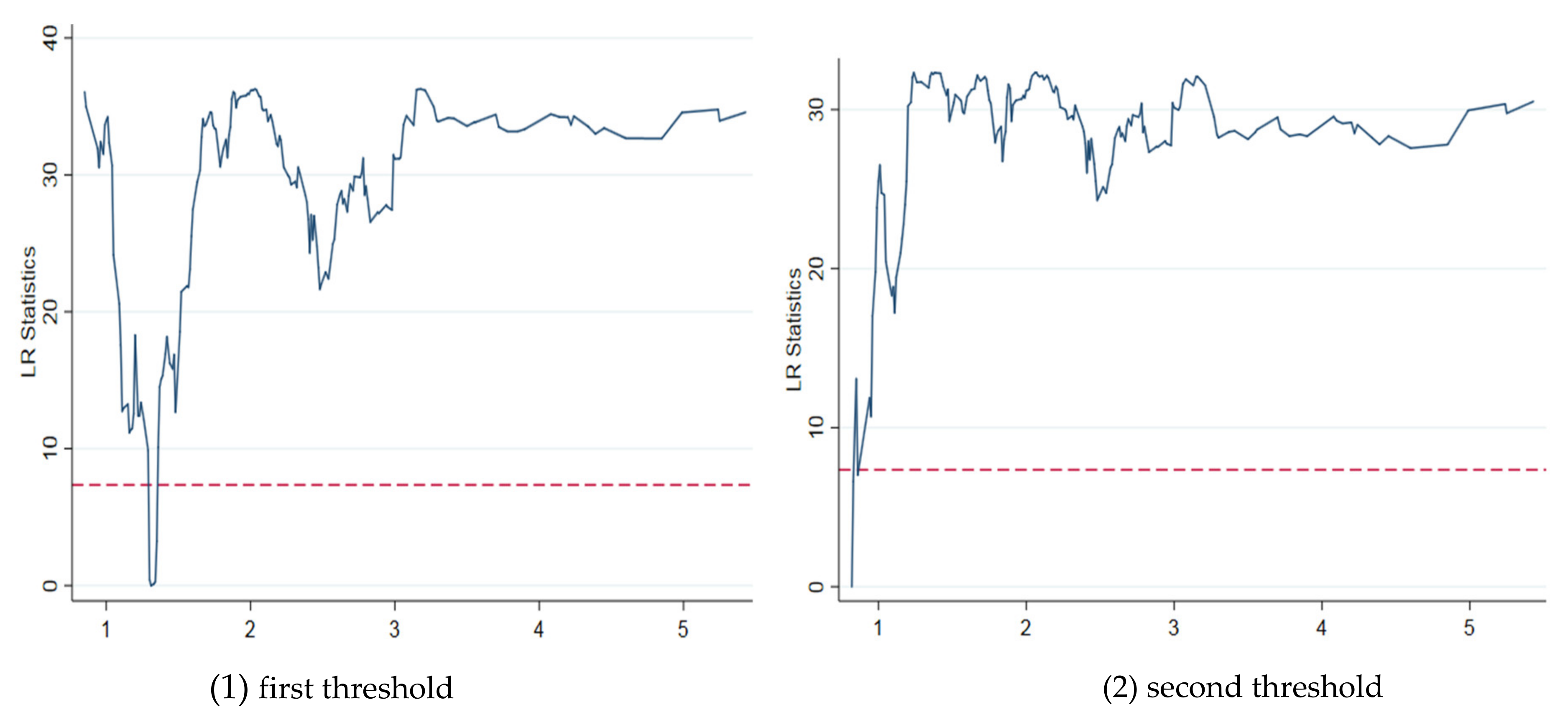
| Threshold value γ1 | 0.82 | [0.817, 0.824] |
| Threshold value γ2 | 1.31 | [1.295, 1.330] |
| Variable | First Interval | Second Interval | Third Interval |
|---|---|---|---|
| 3.4714 *** (4.92) | |||
| 1.088 *** (4.10) | |||
| −2.017 *** (−8.53) | |||
| −133.48 *** (−8.34) | −122.52 *** (−7.31) | −89.15 *** (−5.59) | |
| −0.00004 *** (−3.07) | −0.00004 *** (−3.15) | −0.00004 *** (−3.37) | |
| −0.0428 *** (−3.00) | −0.0357 ** (−2.45) | −0.0174 (−1.28) | |
| 1.827 ** (2.08) | 2.063 ** (2.29) | 3.456 *** (4.09) | |
| 0.0039 ** (2.02) | 0.0035 * (1.78) | 0.0021 (1.18) | |
| −0.6355 *** (−7.83) | −0.4365 *** (−5.54) | −0.2085 ** (−2.58) | |
| Constant term | 4.986 *** (16.62) | 4.603 *** (13.61) | 4.008 *** (12.95) |
| Province effect | yes | yes | yes |
Publisher’s Note: MDPI stays neutral with regard to jurisdictional claims in published maps and institutional affiliations. |
© 2022 by the authors. Licensee MDPI, Basel, Switzerland. This article is an open access article distributed under the terms and conditions of the Creative Commons Attribution (CC BY) license (https://creativecommons.org/licenses/by/4.0/).
Share and Cite
Huo, C.; Chen, L. The Impact of the Income Gap on Carbon Emissions: Evidence from China. Energies 2022, 15, 3771. https://doi.org/10.3390/en15103771
Huo C, Chen L. The Impact of the Income Gap on Carbon Emissions: Evidence from China. Energies. 2022; 15(10):3771. https://doi.org/10.3390/en15103771
Chicago/Turabian StyleHuo, Congjia, and Lingming Chen. 2022. "The Impact of the Income Gap on Carbon Emissions: Evidence from China" Energies 15, no. 10: 3771. https://doi.org/10.3390/en15103771
APA StyleHuo, C., & Chen, L. (2022). The Impact of the Income Gap on Carbon Emissions: Evidence from China. Energies, 15(10), 3771. https://doi.org/10.3390/en15103771