Research on Diagnosis and Prediction Method of Stator Interturn Short-Circuit Fault of Traction Motor

Abstract

The traction motor (TM) is an essential part of the high-speed train, the health condition of which determines the quality and safety of the vehicle. Hence, this study proposed a novel approach to diagnosing and predicting the TM stator interturn short-circuit fault (SISCF). Based on the Park vector (PV) of the stator current, this method could overcome the interference of current sensor errors, null shift, and motor frequency fluctuations in the actual conditions. More specifically, Park’s transformation was used to obtain the PV of the stator current. Then, the PV was fitted to obtain the elliptical trajectory and its parameters from which the negative sequence component of the stator current could be calculated. Finally, the SISCF diagnosis and prediction method were realized by the magnitude and trend of the negative current as well as the inclination of the trajectory ellipse. Furthermore, the performance of the proposed method was validated by a simulation model and a series of experiments. The simulation results were consistent with the experimental results, supporting the validity and correctness of the method proposed in this study.

1. Introduction

With the rapid development of railroad construction, the safety of trains is receiving increasing attention. The traction motor (TM), usually an induction motor, is essential for the train traction system. Once a fault occurs in the TM, it puts the safety of train operations at risk. Stator interturn short-circuit fault (SISCF) is one of the main failures of the TM. Worse still, it can evolve into severe failures, for instance, the phase-to-phase short-circuit fault. Therefore, it is important to research SISCF diagnosis and prediction methods exhaustively.

Electrical and magnetic signals are the two main objects to research the diagnostic and prediction method of SISCF. A motor fault monitoring method was proposed in [1], which depended on the diagonal elements of the negative sequence impedance matrix. It excluded the error of load, operating conditions, and measurements, but required offline parameters and additional equipment. Reference [2] proposed a phasor compensation approach to detect minor interturn short-circuit faults. The study estimated the fault severity of voltage unbalance, sensor errors, and the motor’s asymmetry in structure. However, it was affected by load fluctuations and other asymmetries. In [3], the second harmonic component in the q-axis current was analyzed to monitor the fault, which realized one-turn SISCF detection. However, it worked in steady state only. In [4], the short-time Fourier transform (STFT) was utilized. It added windows to the stator currents and voltages to obtain an STFT spectrum that was used to perform fault diagnosis. However, the STFT cannot consider both time and frequency resolution because the windows cannot be changed once determined. In [5], the slight interturn fault was detected by the proposed condition-monitoring systems based on the discrete wavelet transform (DWT). Although this method could be verified under different loads, there was a lack of experimental verification because it was mainly verified by simulation. In [6], an asymmetric induction machine model-based diagnosis method was proposed, which could eliminate the effects of voltage imbalance and the motor’s inherent asymmetry. However, it is difficult to obtain accurate parameters from an operation motor since the parameters change with load conditions. In [7], a novel approach was proposed based on high-frequency impedance, but it needed to capture both high-frequency phase voltages and currents. In [8,9,10], the air gap magnetic field was monitored by observation coils arranged in the stator slot. When the SISCF occurs, the air gap magnetic field generates specific harmonics, which inducts corresponding electric potentials in the coils. Since this method is an invasive monitoring method, it is not suitable for the motors already in operation as well as the induction motor which typically has a narrow airgap. Machine learning has been widely applied to diagnose SISCF in recent years. Reference [11] proposed a method to analyze the measured signals using the genetic algorithm. Graph-based semi-supervised learning was adopted in [12] to realize online fault identification. In [13], a convolutional neural network-based diagnosis method was employed to detect and classify the stator winding faults. However, these intelligence algorithms need a mass of data to train the model to achieve good results.

Identifying SISCF by electrical signals has good application value because it does not require additional sensors and causes no damage to the motor’s structure. The stator current is the most commonly used signal. Meanwhile, Park’s transform is an effective means to process the three-phase current. Refs. [14,15,16] took the ratio of the dual-frequency component to the fundamental component in the Park vector (PV) as the fault feature. Still, it is not a good indicator of SISCF in the case of a minor fault and heavy load since the fundamental current increases with the load. In [17], the triplet frequency current of phase current and PV’s shape were utilized. However, it took no consideration of the impact of load changes. In [18], the wavelet coefficient which contains the component of 100 Hz was adopted to diagnose SISCF, for the reason that the coefficient amplitude increases when the fault occurs. In addition, Refs. 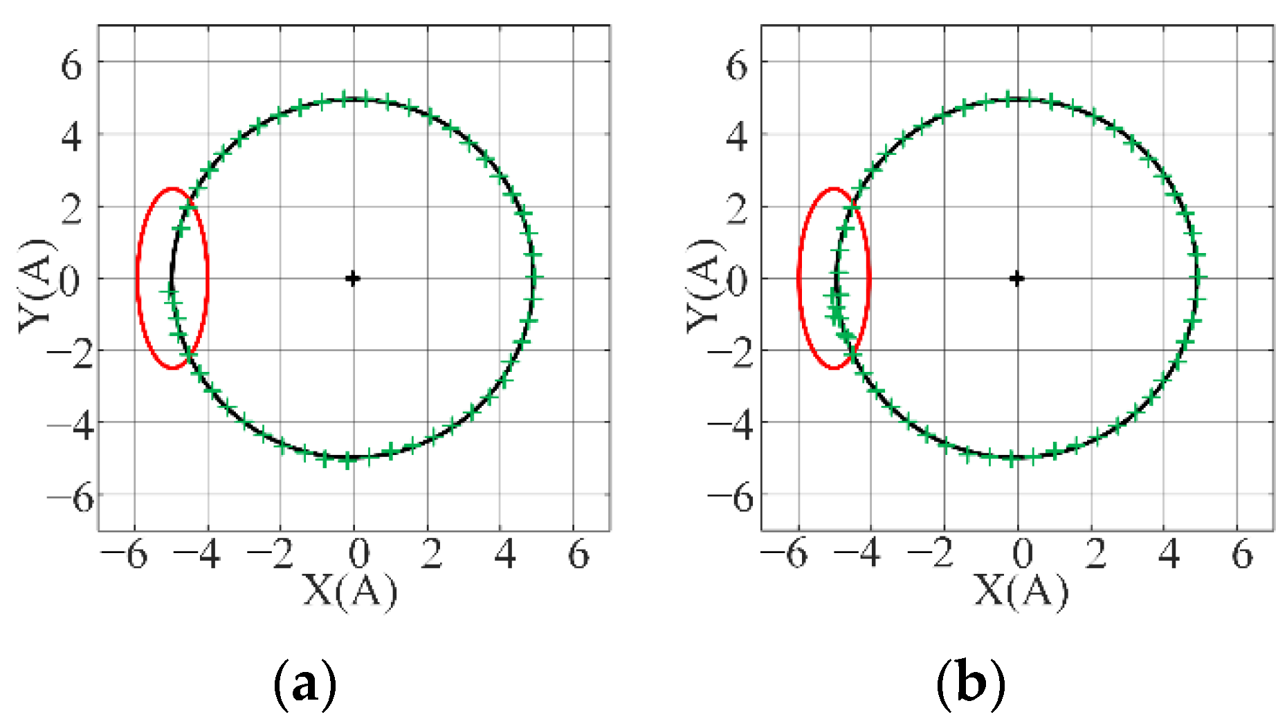[16,17] pointed out that the long and short axis of the Park vector trajectory (PVT) ellipse are correlated with the positive and negative sequence components of the stator current, respectively. Although the studies above have yielded some achievements by Park’s transformation, there are inevitable drawbacks to them which can be expressed as follows.

• Sensor errors and zero drifts were not considered in the previous study. These deviations change the PVT and its modulus, which in turn aggravates the extraction of fault features.
• The frequency of the motor is time-varying, which makes it challenging to obtain the exact double frequency component of the fundamental.

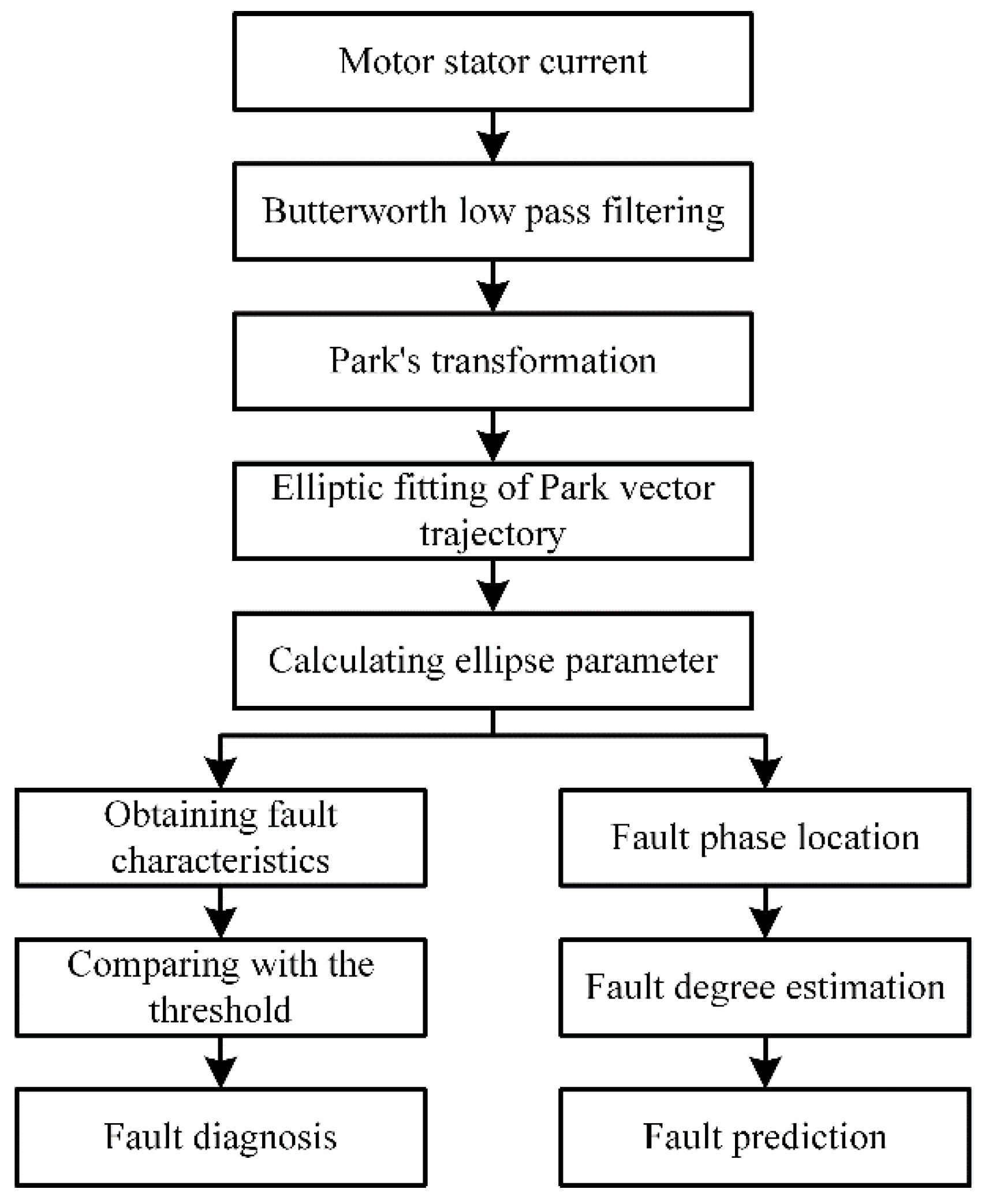
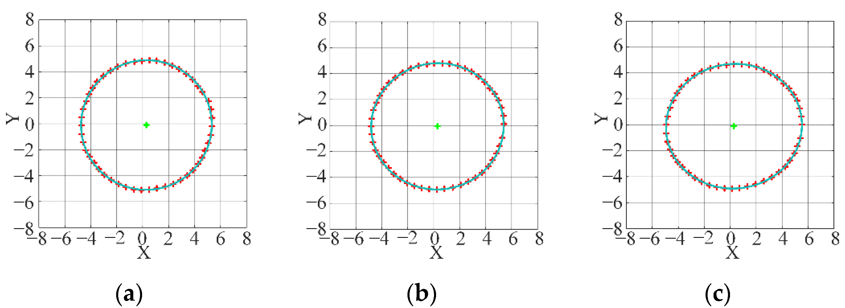
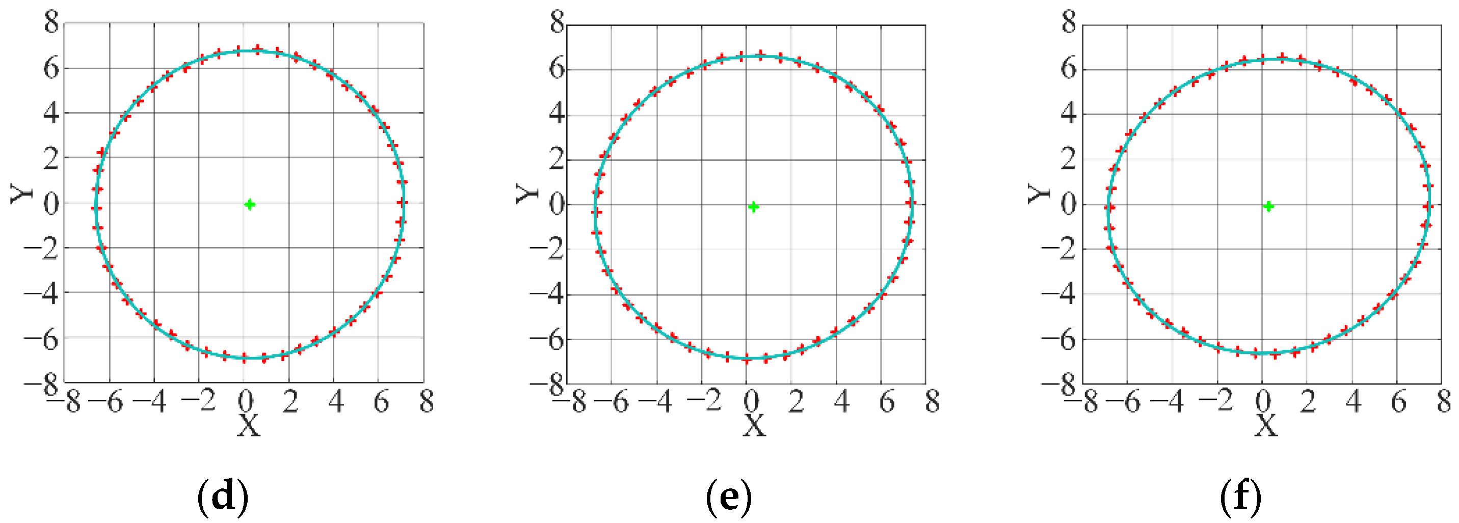
A new approach is proposed to diagnose and predict the SISCF by deriving the relationship between PVT’s ellipse parameters and the stator current’s sequence components. Specifically, Park’s transformation was performed on the stator current to obtain the PVT. Then, the PVT was fitted to the ellipse to obtain the semi-major axis, semi-minor axis, and long axis dip angle parameters. Based on the elliptic coefficient, the negative sequence current was calculated to diagnose the SISCF. Then, the negative current and long axis dip angle were applied in prediction. Finally, a simulation model and an experimental platform were built to verify the proposed method. The simulation results were consistent with the experimental results, indicating the correctness and effectiveness of the proposed technique.

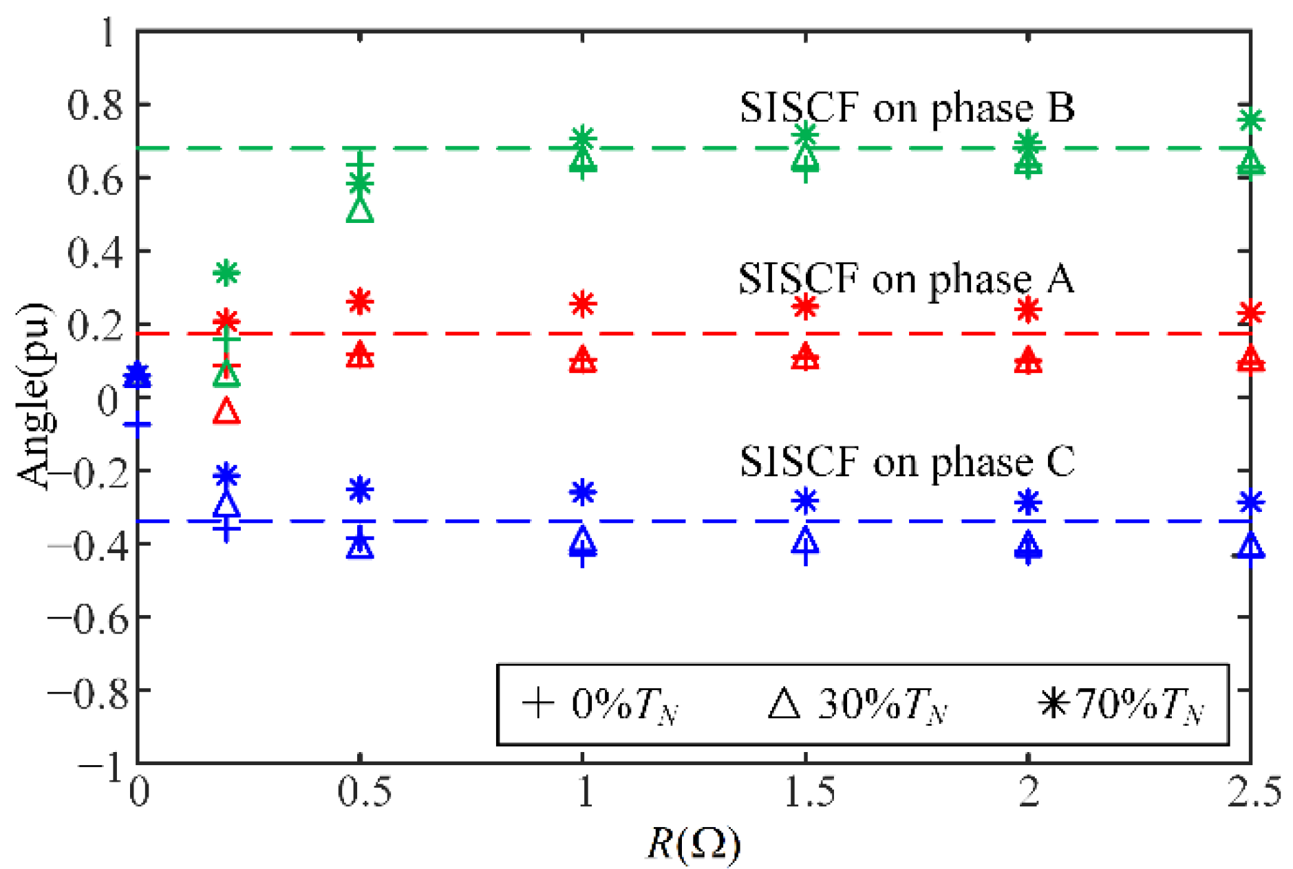
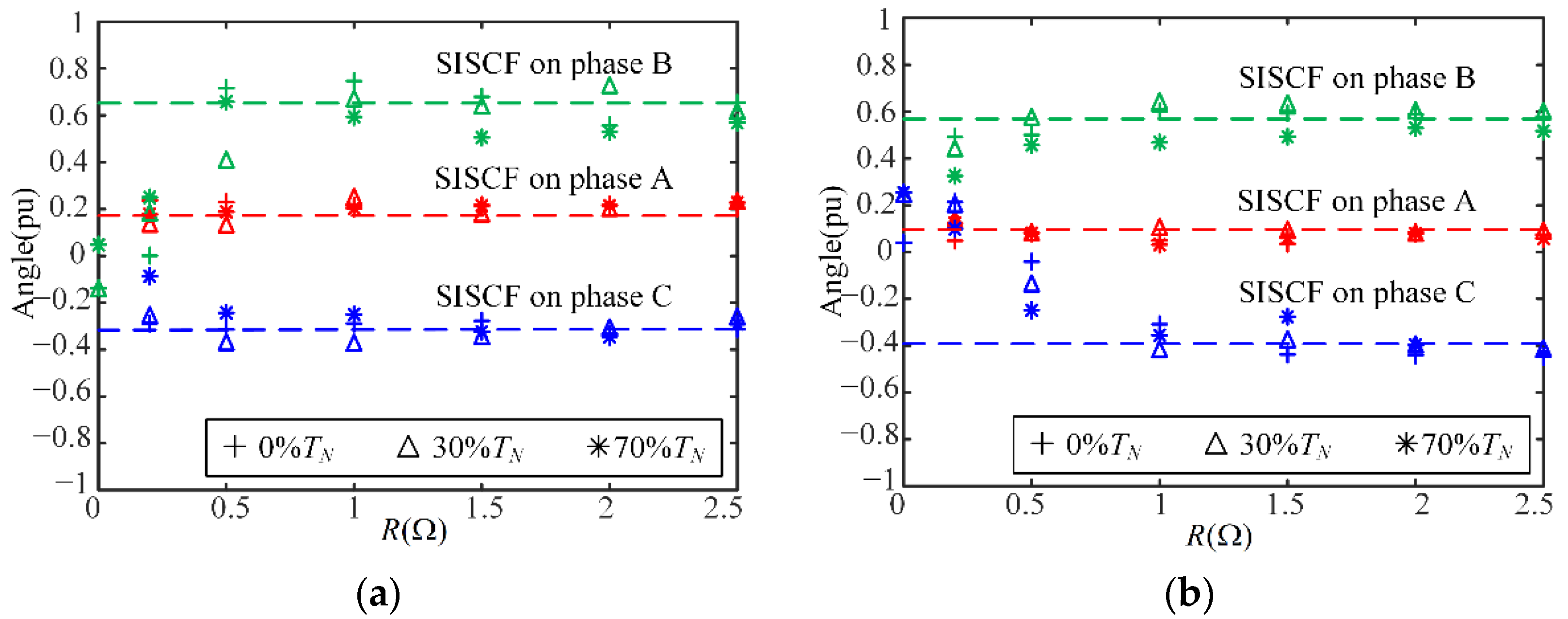
This article is organized as follows. Section 2 presents the fault characteristics of the TM with SISCF. In Section 3, the theory and steps of the diagnosis and prediction method are introduced. In addition, the negative current is adopted to indicate the severity of SISCF and the long axis dip angle to the fault phase location. 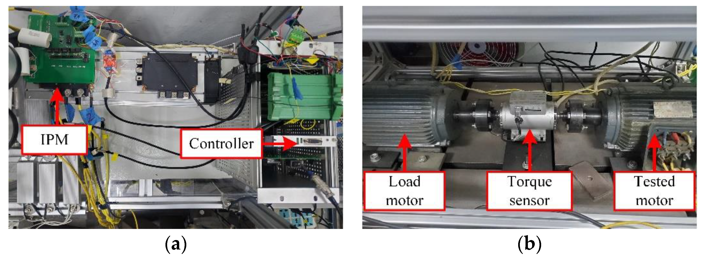Section 4 is the simulation analysis of the diagnostic and prediction approach, and Section 5 shows the experimental verification. Finally, the conclusions of this paper are drawn in Section 6.

2. Traction Motor Stator Interturn Short-Circuit Fault Characters

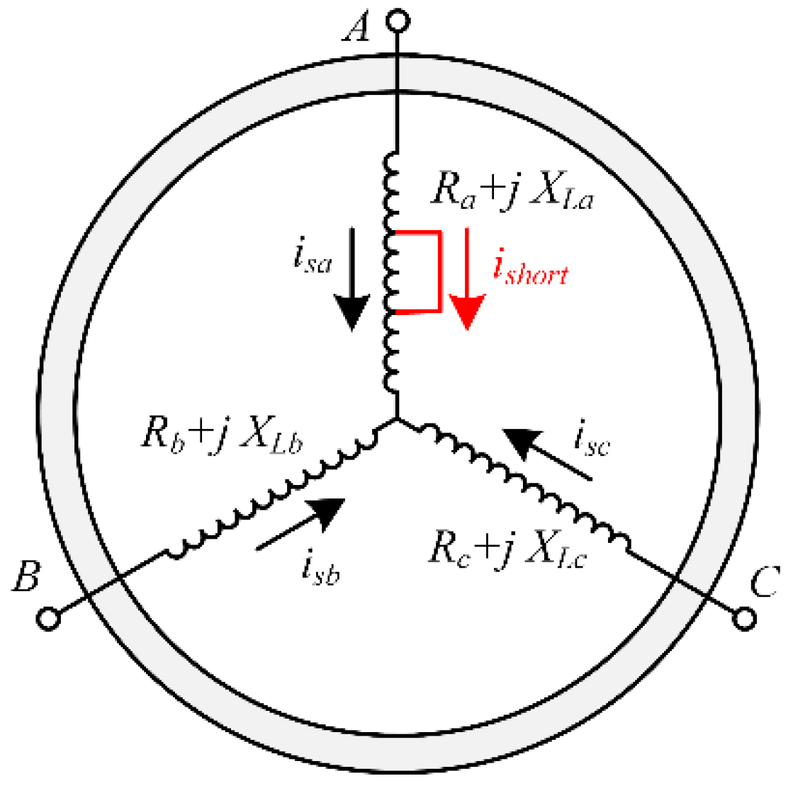
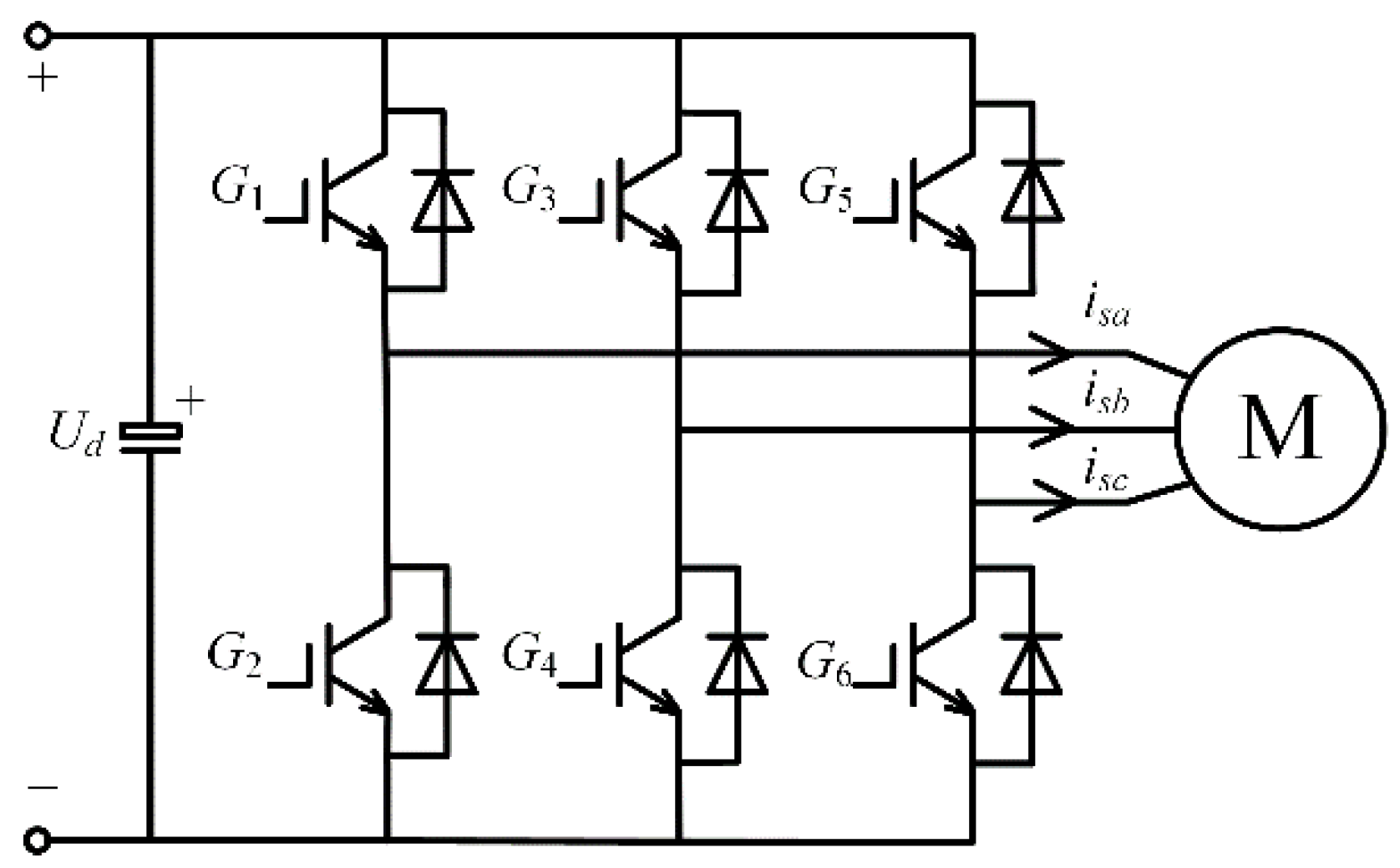
The stator windings are symmetrically distributed when the TM is normal. While the SISCF occurs, the symmetry is destroyed. The schematic diagram of the SISCF is shown in Figure 1. The three-phase stator winding impedances of the healthy motor are equal to each other. However, if the motor stator is at fault, the stator winding impedance changes. The three-phase symmetrical voltage acting on the asymmetrical stator impedance results in negative sequence currents.

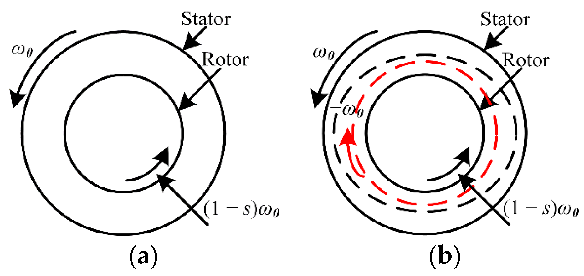
If the stator winding is asymmetrical, the air gap magnetic potential changes from circular to elliptical. Subsequently, the elliptical airgap magnetic potential can be decomposed into two components. The forward component is denoted as F₁₁, and the reverse is F₁₂. The two parts have the same rotational speed. Under the forward component F₁₁, the voltage potential and current with frequency sf₀ are induced in the rotor winding. Further, the rotor current generates a rotor magnetic potential F₂₁, which remains stationary with F₁₁. The forward component generates a constant forward electromagnetic torque T₁. 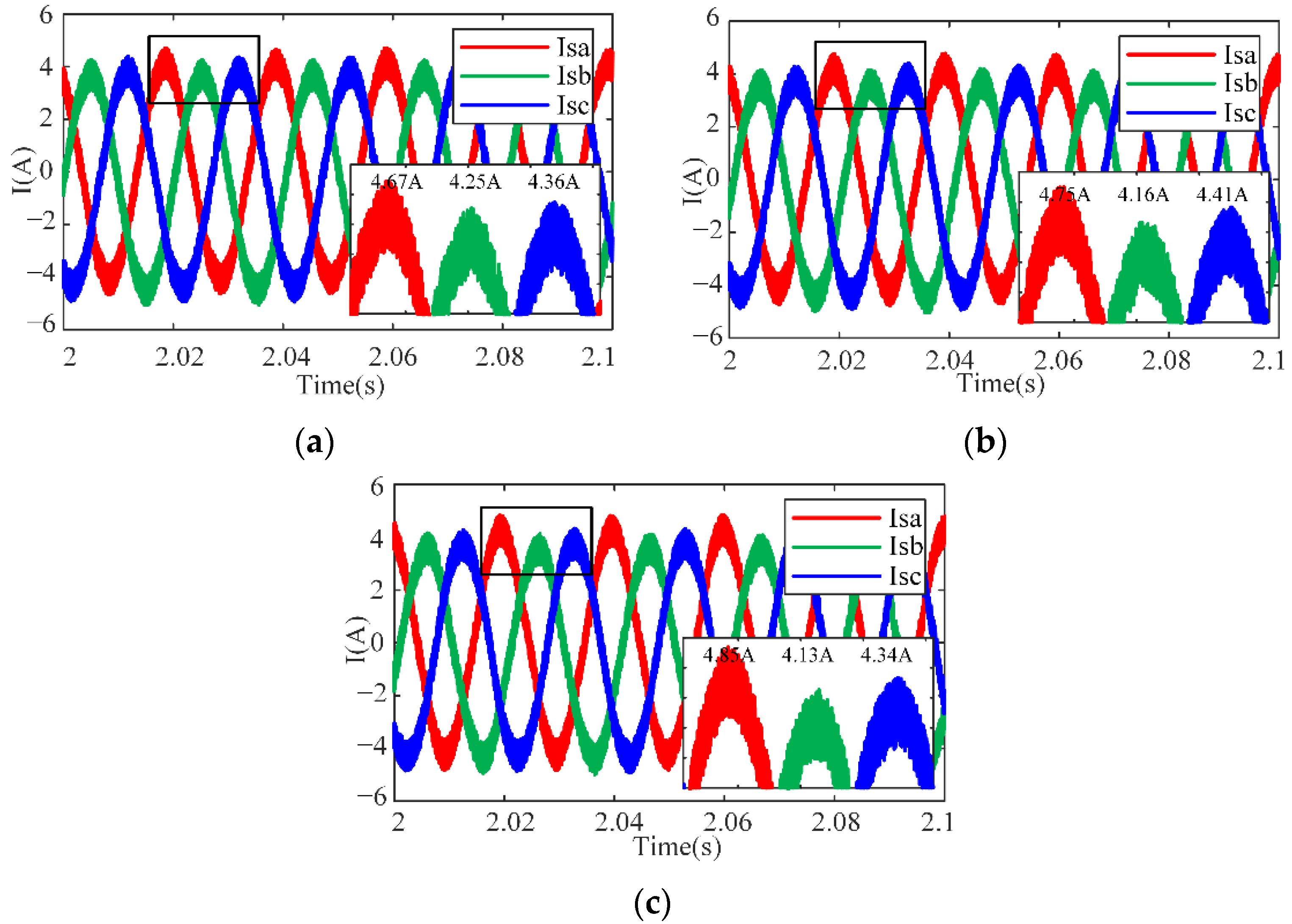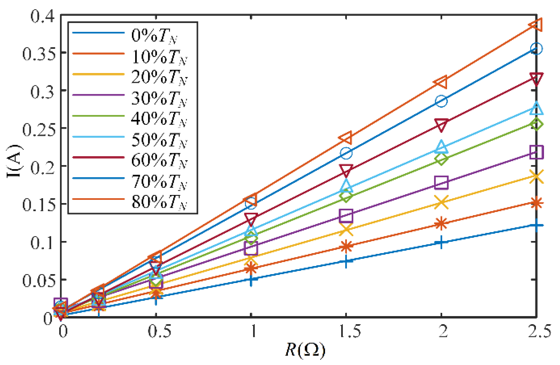However, under the action of the reversed component F₁₂, the AC potential induced in the stator windings causes the negative sequence component in stator currents. It is evident that the deeper the fault, the larger the value of the negative sequence component, as shown in Figure 2.

3. Fault Diagnosis and Prediction Method Based on Park’s Transformation and Ellipse Fitting

3.1. Park’s Transformation

The coordinate transformation has unique superiority in analyzing the dynamic characteristics of motors. As a result, more and more experts have applied it to motor fault diagnosis. Park’s transformation has been thoroughly studied and widely used [16,19].

The transformation matrix of the three-phase stationary coordinate system (ABC) to the two-phase static coordinate system (αβ) is given as

$$\left[\begin{array}{l}{i}_{s\alpha }\\ i_{s\beta }\end{array}\right]=\sqrt{\frac{2}{3}}\left[\begin{array}{ccc}1& -\frac{1}{2}& -\frac{1}{2}\\ 0& \frac{\sqrt{3}}{2}& -\frac{\sqrt{3}}{2}\end{array}\right]\left[\begin{array}{c}{i}_{sa}\\ i_{sb}\\ i_{sc}\end{array}\right].$$

(1)

The TM is driven by an inverter, and thus it is supposed that the three-phase voltage is symmetrical. In such a situation, the effect of voltage asymmetry is ignored. Moreover, it is assumed that the TM is symmetrical, and the three-phase stator current contains only the fundamental wave with frequency f₀. The three-phase stator current is expressed as

$$i_{sa}=I_1\cos ({\omega }_{0}t-{\alpha }_1),$$

(2)

$$i_{sb}=I_1\cos ({\omega }_{0}t-{\alpha }_1-\frac{2\pi }{3}),$$

(3)

$$i_{sc}=I_1\cos ({\omega }_{0}t-{\alpha }_1+\frac{2\pi }{3}),$$

(4)

where I₁ is the amplitude of the fundamental wave, ω₀ is the angular frequency of the fundamental wave, and α₁ is the phase angle of the fundamental.

The three-phase stator currents are converted by the conversion matrix and expressed as

$$i_{s\alpha }=\sqrt{\frac{2}{3}}{i}_{sa}-\frac{1}{\sqrt{6}}{i}_{sb}-\frac{1}{\sqrt{6}}{i}_{sc}=\sqrt{\frac{3}{2}}{I}_1\cos ({\omega }_{0}t-{\alpha }_1),$$

(5)

$$i_{s\beta }=\frac{1}{\sqrt{2}}{i}_{sb}-\frac{1}{\sqrt{2}}{i}_{sc}=\sqrt{\frac{3}{2}}{I}_1\sin ({\omega }_{0}t-{\alpha }_1).$$

(6)

The PV is defined as the synthetic vector of i_sα and i_sβ:

$$l=i_{s\alpha }+j{i}_{s\beta }.$$

(7)

L is the modulus value of the PV and is expressed as

$$L=\sqrt{i_{s\alpha }^2+i_{s\beta }^2}=\sqrt{\frac{3}{2}}{I}_1.$$

(8)

The stator current of the healthy TM is transformed into a DC component of L by Park’s transformation. The value of L is equal to the radius of the PVT.

Once the SISCF occurs, the stator current is expressed as a superposition of the positive and negative sequence components, which is given as

$$i_{sa}=I_1\sin ({\omega }_{0}t-{\alpha }_1)+I_{-}\sin (-{\omega }_{0}t-{\alpha }_{-}),$$

(9)

$$i_{sb}=I_1\sin ({\omega }_{0}t-{\alpha }_1-\frac{2\pi }{3})+I_{-}\sin (-{\omega }_{0}t-{\alpha }_{-}-\frac{2\pi }{3}),$$

(10)

$$i_{sc}=I_1\sin ({\omega }_{0}t-{\alpha }_1+\frac{2\pi }{3})+I_{-}\sin (-{\omega }_{0}t-{\alpha }_{-}+\frac{2\pi }{3}),$$

(11)

where I₁ is the amplitude of positive current, I_– is the amplitude of negative sequence current, and α₁ and α_– are the phase angle of positive and negative sequence current, respectively.

Based on Park’s transform, the three-phase stator current is converted into

$$i_{s\alpha }=\sqrt{\frac{3}{2}}{I}_1\sin ({\omega }_{0}t-{\alpha }_1)+\sqrt{\frac{3}{2}}{I}_{-}\sin (-{\omega }_{0}t-{\alpha }_{-}),$$

(12)

$$i_{s\beta }=\sqrt{\frac{3}{2}}{I}_1\cos ({\omega }_{0}t-{\alpha }_1)+\sqrt{\frac{3}{2}}{I}_{-}\cos (-{\omega }_{0}t-{\alpha }_{-}).$$

(13)

Therefore, L is expressed as

$$L=\sqrt{\frac{3}{2}(I_1^2+I_{-}^2)+3I_1{I}_{-}\cos (2{\omega }_{0}t-{\alpha }_1+{\alpha }_{-})}.$$

(14)

The PVT changes into an ellipse from a circular form. The semi-major and semi-minor axis of the ellipse are denoted as

$$a=l_{\max }=\sqrt{\frac{3}{2}(I_1^2+I_{-}^2)+3I_1{I}_{-}},$$

(15)

$$b=l_{\min }=\sqrt{\frac{3}{2}(I_1^2+I_{-}^2)-3I_1{I}_{-}},$$

(16)

where a is the semi-major axis of the ellipse and b is the semi-minor axis.

Finally, the amplitudes of the positive sequence and the negative sequence are expressed as

$$I_1=\sqrt{\frac{1}{6}}(a+b),$$

(17)

$$I_{-}=\sqrt{\frac{1}{6}}(a-b).$$

(18)

From (17) and (18), it can be concluded that the positive sequence is proportional to the sum of a and b, and the negative sequence is proportional to the difference between the semi-major and semi-minor axis.

3.2. Ellipse Fitting Based on the Least Square Method

The general equation of the ellipse contains five coefficients A, B, C, D, and E, which can represent any ellipse in the plane, and its algebraic expression is

$$x^2+Axy+B{y}^2+Cx+Dy+E=0.$$

(19)

Based on the coefficients in (19), the semi-major axis, semi-minor axis, and the long axis inclination angle can be calculated. The parameters are expressed as

$$a=\sqrt{\frac{2(ACD-B{C}^2-D^2+4BE-A^{2}E)}{(A^2-4B)(B+1-\sqrt{A^2+{(1-B)}^2})}},$$

(20)

$$b=\sqrt{\frac{2(ACD-B{C}^2-D^2+4BE-A^{2}E)}{(A^2-4B)(B+1+\sqrt{A^2+{(1-B)}^2})}},$$

(21)

$$\theta =\frac{1}{2}\arctan \frac{B}{A-C}.$$

(22)

The least square method is a common approach for fitting ellipses, which minimizes the sum of squares of measurement errors when the errors are normally distributed [20,21]. The objective function is

$$F(A,B,C,D,E)={\displaystyle \sum _{i=1}^n{(x_i^2+A{x}_i{y}_i+B{y}_i^2+C{x}_i+D{y}_i+E)}^2},$$

(23)

where n is the number of sampling points.

In order to avoid a zero solution, the constraint is given as

$$A+C=1.$$

(24)

The coefficients are determined by calculating the minimum value of the objective function. According to the extreme value principle, the partial derivatives for each coefficient of the objective function are calculated. The expression is

$$\frac{\partial F}{\partial A}=\frac{\partial F}{\partial B}=\frac{\partial F}{\partial C}=\frac{\partial F}{\partial D}=\frac{\partial F}{\partial E}=0.$$

(25)

The above equation is a system of linear equations. The unknown coefficients can be found by solving (24) and (25).

3.3. Traction Motor Stator Interturn Short-Circuit Fault Diagnosis and Prediction Method

In the actual working condition, diagnosis and prediction of the SISCF are affected by the following problems. Firstly, the current sensor is affected by errors and zero offsets, which result in deviations in the sampled current signals. The errors further result in a deviation between the geometric center of the PVT and the coordinate axis origin. This deviation leads to fluctuations in the trajectory modulus. Secondly, the motor’s operating frequency is not constant but fluctuates around the target frequency because of disturbance and control system performance. It is difficult to obtain the exact diphasic fundamental frequency component of the PV, which limits the application of diphasic component-based methods. Finally, the TMs, especially motors on high-speed trains, have a high operation frequency. When the TM operates at a high frequency, the sampling data per motor cycle decline, which leads to a deviation between the maximum and minimum values of the PV obtained from the sampling data and the actual data.

The method of elliptical fitting to the PVT overcomes the above problems. Firstly, ellipse fitting can smooth the PVT, which helps to reduce the impact of sensor errors. Secondly, calculating the semi-major and semi-minor axis of the PVT from the elliptic parameters overcomes the sensor null shift problem regarding the elliptical geometric center. In the end, ellipse fitting can obtain accurate fitting curves even though the motor frequency is unstable. Figure 3 shows the ellipse of the PVT when there are fluctuations in motor frequency and PVT modulus.

A simulation was performed to verify the advantage of the ellipse fitting method in calculating the sequential current. Taking into account the errors and null shifts of the data acquisition system in the experiment, the simulation conditions were set as follows. The sampling error was ±0.5 A-distributed random number. The null shift was −0.41 A for the B phase sensor and −0.28 A for the C phase. The series resistance was connected in phases B and C to simulate an unbalanced fault. The simulation data are shown in

Table 1. Comparison of different methods for calculating negative sequence current.

Load Level and Fault Degree	Real Data	Ellipse Fitting Method	Direct Calculation
30% TN, 0 Ω	0.0170 A	0.0159 A	0.2815 A
30% TN, 1 Ω	0.0917 A	0.0893 A	0.2996 A
30% TN, 2 Ω	0.1787 A	0.1805 A	0.3763 A
70% TN, 0 Ω	0.0144 A	0.0125 A	0.2936 A
70% TN, 1 Ω	0.1512 A	0.1489 A	0.3636 A
70% TN, 2 Ω	0.2862 A	0.2875 A	0.4989 A

, where the real data are the actual negative sequence currents in the stator currents. After filtering the sampled signals, the ellipse fitting method and direct calculation were utilized to obtain negative currents, respectively. It can be concluded from Table 1 that the ellipse fitting method proposed in this paper could overcome the influence of sensor error and zero drift and accurately extract the negative sequence current.

The ellipse fitting method to the PVT has advantages in obtaining the fault features from stator currents. The detailed steps of SISCF diagnosis and prediction are shown in Figure 4.

4. Simulation Analysis

A TM simulation model was built by Matlab/Simulink.

Table 2. Induction motor simulation parameters.

Parameters	Values
Inverter DC voltage Ud (V)	540
Rated power PN (kW)	2.2
Rated voltage UN (V)	380
Rated current IN (A)	4.25
Rated Speed (r/min)	1420
Rated efficiency ηN	78.65%
Rated torque TN (N·m)	14.795
Rated speed nN (r/min)	1420
Power Factor cosφ	0.85
Number of pole pairs P	2
Stator resistance Rs (Ω)	2.602
Rotor resistance Rr (Ω)	1.200

records the induction motor’s parameters, and the main circuit topology of the model is shown in Figure 5. The SISCF is a kind of stator unbalanced fault, which leads to stator impedance asymmetry. It has been demonstrated in [22] that the stator side impedances placed inside and outside the motor are equivalent to the stator current characteristics when simulating a SISCF. In the case of minor SISCF, a small number of short circuit turns and large equivalent resistance of short circuit point, it is assumed that the stator inductance changes little and can be ignored. Therefore, the SISCF can be simulated by connecting resistances outside the stator, where the resistances of the series connection are far less than the stator impedance. The slight SISCF simulation is achieved by connecting resistors in series with two of the three phases in the stator without destroying the motor in this study.

4.1. Fault Diagnosis Simulation and Analysis

The error and zero drift of the current sensor were considered in the simulation, and the parameters were set as follows. The sampling error was fixed to ±0.5 A, and null shifts were −0.41 A for the B phase sensor and −0.28 A for the C phase sensor. The operating frequency is 50 Hz. Figure 6 shows stator currents at light load. Figure 6a shows the current of a healthy motor, Figure 6b shows the fault currents of the B and C phase with 1 Ω resistors in series, and Figure 6c shows the case of 2 Ω resistors in series. It is obvious that the currents were symmetrical when the TM was normal. However, if the motor was faulty, the currents became asymmetrical. The more serious the fault, the greater the three-phase current imbalance.

Figure 7 shows the PVTs and their fitted ellipse curves, where Figure 7a–c are the PVTs and fitted curves for the normal TM, the motor with 1 Ω resistors in series in phases B and C, and 2 Ω resistors in series in phases B and C, respectively, under light load. Figure 7d–f are PVTs and curves under heavy load with the same degree of failure as in Figure 7a–c separately. It was found that the difference between the elliptic semi-major and semi-minor axis increased with the growth of the fault severity in comparison with Figure 7a–c. The pattern of changes was the same in Figure 7d–f, which suggests that the negative current increased. When the load increased, the fundamental current increased, which enlarged both semi-major and semi-minor axis of the ellipse. In other words, the fundamental current increased while the negative current changed slightly. In addition, the center of the ellipse deviated from the coordinate origin due to the zero drifts of current sensors.

The negative sequence current was calculated according to (18), and the data are shown in

Table 3. Simulation data of motor negative sequence current.

Load Level	Values of Resistances in Series in B and C Phases
	0 Ω	1 Ω	2 Ω
0% TN	0.0064 A	0.0501 A	0.0990 A
30% TN	0.0159 A	0.0893 A	0.1805 A
70% TN	0.0125 A	0.1489 A	0.2875 A

. Due to the asymmetry of the TM, there was a small negative sequence current in the healthy motor. When the TM had a SISCF, the symmetry of the motor was broken, which led to a significant negative sequence component in the stator current. As the severity of the fault increased, the negative sequence current became more prominent. The negative sequence current increased slightly with the rise in load under the same fault degree. Therefore, it could be correctly diagnosed by setting a suitable threshold and combining it with load conditions.

4.2. Fault Prediction Simulation and Analysis

The simulation was carried out at various load levels and different fault degrees. And the operating frequency is 50 Hz. The prediction steps were as follows. Firstly, ellipse fitting was performed to the PVT to obtain the stator negative sequence current under various conditions. Secondly, in order to get the changing trend, a polynomial was fitted to the negative current. Finally, the prediction of the SISCF could be achieved by the change tendency and fault phase location technique.

Figure 8 shows the data of the negative sequence current of the motor stator under different loads and fault conditions. The fault data were polynomial fitted to obtain their relationship with the change in the fault degree, and the fitted curve is also shown in Figure 8. The data showed that the negative sequence current increased linearly with the fault level, and the slope of the curve grew as the load increased. According to the relationship, the extent of the fault could be predicted by the negative sequence current.

When a SISCF occurs in a motor, the current in the short-circuiting phase is the largest and currents in the sound phases are smaller. In addition, the windings of the motor have different spatial distributions. Therefore, the inclination of the PVT ellipse’s long axis varies when the fault happens in different phases. Figure 9 shows the inclination distributions. It can be seen from Figure 9 that the distribution of the long axis inclination was different when the failure occurred in the A, B, and C phases. When the faults occurred in the same phase, the dip angle converged to the same value. Consequently, the fault phase could be located based on the long axis tilt angle.

4.3. Fault Diagnosis and Prediction Method Validation at Low and Medium Frequency

The traction motor possesses a wide operating frequency and sometimes works at low and medium frequency conditions. The PVT can be accurately fitted by appropriately changing the number of sampling points when the motor's working frequency changes. In order to verify the adaptability of the proposed method under different operating frequencies, simulations are carried out at low and medium frequencies respectively.

Table 4. Simulation data of motor negative sequence current at 10 Hz.

Load Level	Values of Resistances in Series in B and C Phases
	0 Ω	1 Ω	2 Ω
0% TN	0.0048 A	0.0275 A	0.0536 A
30% TN	0.0110 A	0.0480 A	0.1066 A
70% TN	0.0158 A	0.0568 A	0.1674 A

records the simulation data of negative current when the motor works at 10 Hz, and

Table 5. Simulation data of motor negative sequence current at 30 Hz.

Load Level	Values of Resistances in Series in B and C Phases
	0 Ω	1 Ω	2 Ω
0% TN	0.0057 A	0.0349 A	0.0704 A
30% TN	0.0138 A	0.0678 A	0.1404 A
70% TN	0.0244 A	0.1048 A	0.2036 A

is the 30 Hz condition. From Table 4 and Table 5, it can be seen that the amplitude of negative sequence current grows with the increase of fault severity and load. The change tendency of negative sequence current is consistent with the rated frequency condition.

Figure 10 shows the negative sequence currents at different load and fault degrees. Figure 10a shows the negative current when the motor works at 10 Hz, and (b) is the 30 Hz condition. Under low and medium frequency conditions, the negative sequence current increases linearly with the fault severity which is consistent with the rated frequency condition. The difference between different frequencies is the amplitude of negative sequence current. When the operating frequency is lower than 50 Hz, the amplitude of negative sequence current decreases.

Figure 11 shows the distributions of the elliptical long axis inclination angle with different fault phases, where (a) is the case of working at 10 Hz and (b) is at 30 Hz. When the fault occurs in the same phase, with the fault severity increasing, the long axis inclination angle approaches the same value.

5. Experimental Validation

An experimental platform was built to verify the correctness and effectiveness of the diagnosis and prediction method. The circuit topology of the platform is shown in Figure 5, and Figure 12 displays the physical parts. The parameters of the experimental platform were consistent with those of the simulation, and the same applies for the fault diagnosis method and prediction steps. The operating frequency is set to 50 Hz for experimental verification.

5.1. Experiments of Motor Fault Diagnosis

Figure 13 records the stator current at different fault degrees when the motor runs at a 30% T_N. Figure 13a shows three-phase currents of the normal TM, while (b) shows the currents of the B and C phase with 1 Ω resistors in series, and (c) is in the case of 2 Ω resistors in series. The unbalance of the currents grew with the fault severity increasing. The fault-phase current was the greatest among the three-phase currents, which is consistent with the simulation results.

Figure 14 shows the stator currents’ PVTs and their fitted ellipses of the SISCF experiment. Due to the slight asymmetry in the motor, there is a small negative sequence current in the healthy condition. So, the PVT showed an elliptical shape, as shown in Figure 14a,d. The eccentricity of the ellipse increased as the fault severity increases. And the difference between the semi-major axis and the short one grows, which indicated an increase in the negative sequence component of the stator current.

Table 6. Experimental data of motor negative sequence current.

Load Level	Values of Resistances in Series in B and C Phases
	0 Ω	1 Ω	2 Ω
0% TN	0.0314 A	0.1543 A	0.2525 A
30% TN	0.0390 A	0.1848 A	0.2986 A
70% TN	0.0511 A	0.2032 A	0.3459 A

records the negative sequence components in stator currents at different loads and fault degrees. There was a small negative sequence current in the normal TM. While the SISCF happened, the negative current increased sharply. The negative sequence current increased slightly with the load growing, which shows the same trend as the simulation. Therefore, the SISCF diagnosis could be achieved by setting a suitable fault threshold combined with the load level. It was shown in the experimental results that the proposed method could effectively extract the negative sequence current to realize the SISCF diagnosis.

5.2. Comparison between the Method Based on Ellipse Fitting and the Method Based on Fundamental Frequency Doubling Component

It could be found from the comparison between (8) and (14) that the double frequency component appears in the Park vector modulus when the SISCF happens. The core of the method based on the double frequency of the fundamental wave is to obtain the amplitude of the double frequency component. For example, if the fundamental frequency is 50 Hz, the amplitudes of the 100 Hz component in the PV need to be calculated.

The spectrum analysis was carried out on the experimental data to obtain the double frequency component.

Table 7. The amplitude of the 100 Hz component based on spectrum analysis.

Load Level	Values of Resistances in Series in B and C Phases
	0 Ω	1 Ω	2 Ω
0% TN	0.0267 A	0.0131 A	0.2287 A
30% TN	0.0061 A	0.0330 A	0.2378 A
70% TN	0.0070 A	0.2093 A	0.1389 A

records the amplitude of the 100 Hz components in Park vector modulus. It was found that the amplitudes of some 100 Hz components did not increase significantly under SISCF, which is inconsistent with the theory, as shown in the red font data. The reason is that the double frequency is not exactly 100 Hz. For example, the actual double frequency of 2 Ω, 70% T_N condition is 97.4 Hz, and the real data is 0.3657 A. The method based on the double frequency component has defects in obtaining the accurate frequency components. Compared with Table 6, the proposed method did not have the problem of inaccurate calculation due to frequency fluctuations.

5.3. Experiments for Motor Fault Prediction

To realize the fault prediction, the negative sequence currents at different fault levels and under various load conditions were analyzed. A polynomial was fitted to the negative sequence current as with the simulation. The curves are shown in Figure 15.

From the curves in Figure 15, the negative sequence current increased linearly with the fault severity. Besides, the negative sequence current slightly increased with the load level, which resulted in a larger slope of the fitted line. Consequently, the prediction of the fault degree could be realized by the negative sequence current with the help of the relationship. The physical TM was more asymmetrical than the model, which resulted in more extensive experimental negative sequence currents than the simulation results under the same conditions. The simulation and experiment results are consistent, which verifies the effectiveness of the proposed fault prediction method.

The relationship between the long axis inclinations of the PVT and the fault phases is shown in Figure 16. Because of the different spatial positions of stator phase windings, the PVT ellipse long axis inclination angles were different when the SISCF occurred in various phases. The inclination angles of the long axis tended to have the same value if the faults occur in the same phase. The experimental results are consistent with the simulation. Therefore, the fault phase could be located according to the long axis tilt angle.

6. Conclusions

In this work, the prediction and diagnosis of SISCF were successfully achieved. A novel approach was proposed based on the relationship between geometric characteristics of PVT and fault characters of the TM. This paper accomplished the following work.

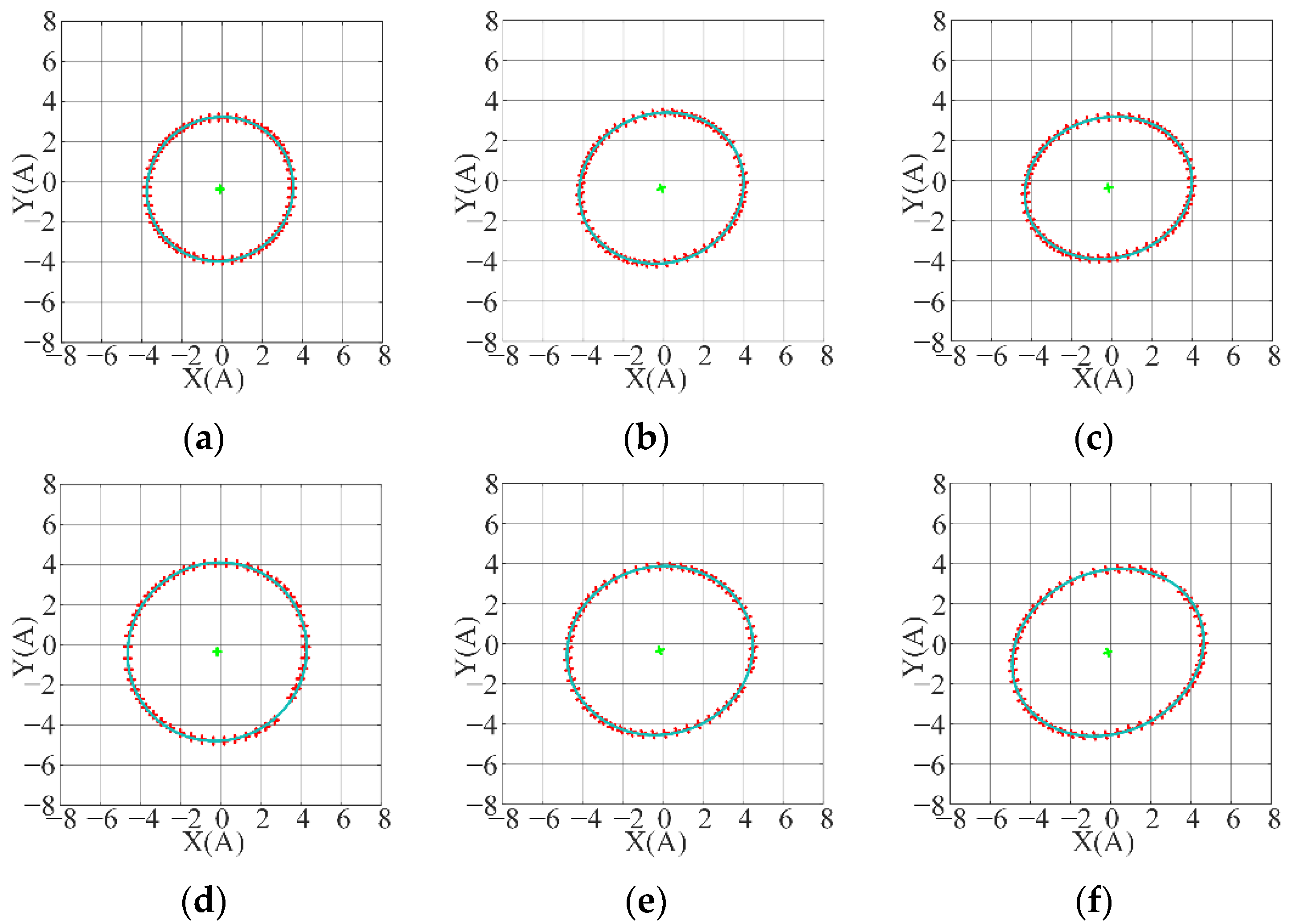
The ellipse was fitted to the PVT of the stator current to obtain elliptical parameters by the least square method. The negative sequence current in the stator was derived by the parameters. This method could overcome the problems of sensor errors, zero drifts, and motor frequency fluctuations.

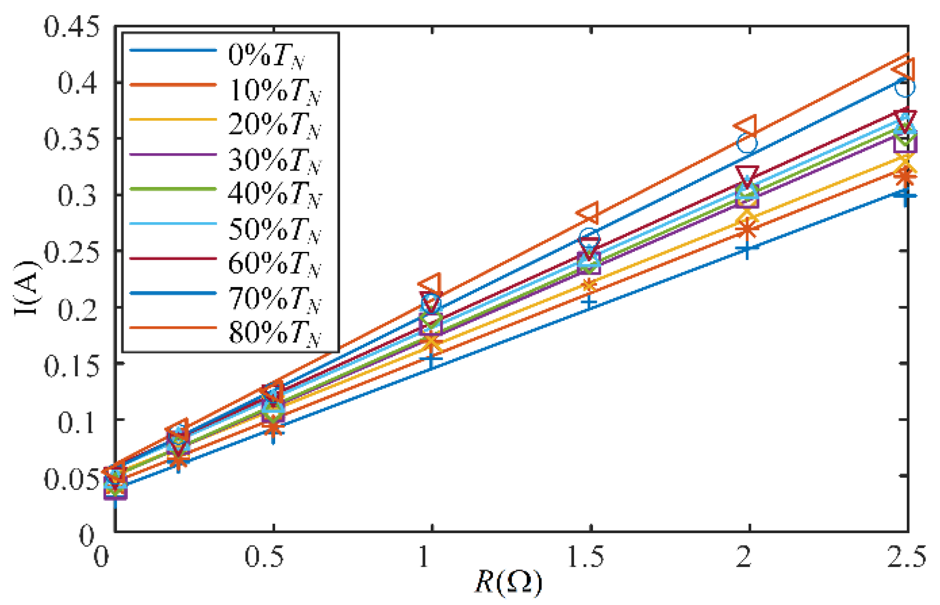
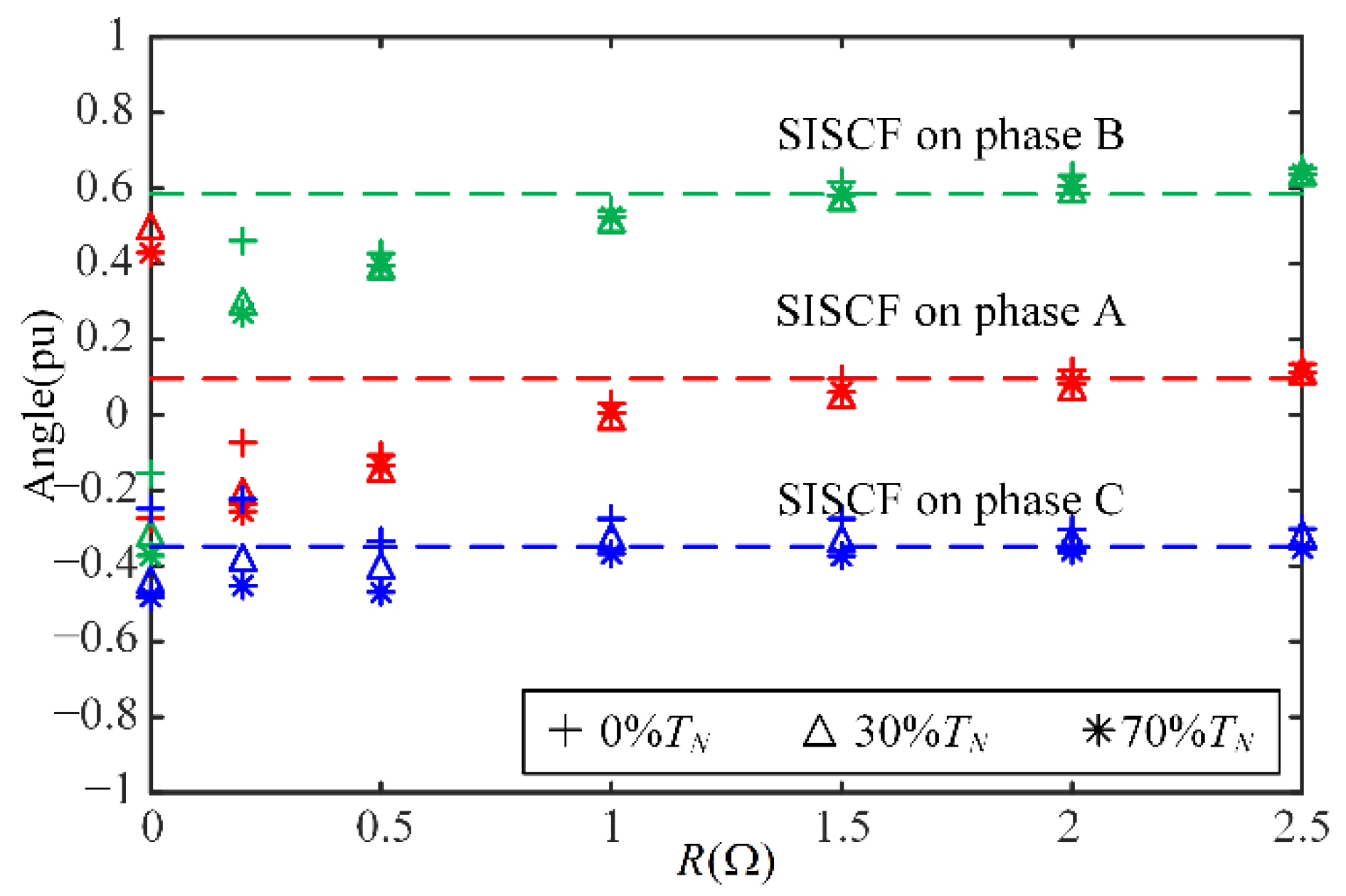
The SISCF diagnosis was achieved based on the negative sequence current. The polynomial fitting was performed to the negative sequence current to get the relationship between the current and fault degrees at different load levels. The prediction of fault, which contains fault degree prediction and fault phase location, was achieved by the combination of the trend of the negative sequence current and inclination angle of the ellipse major axis.

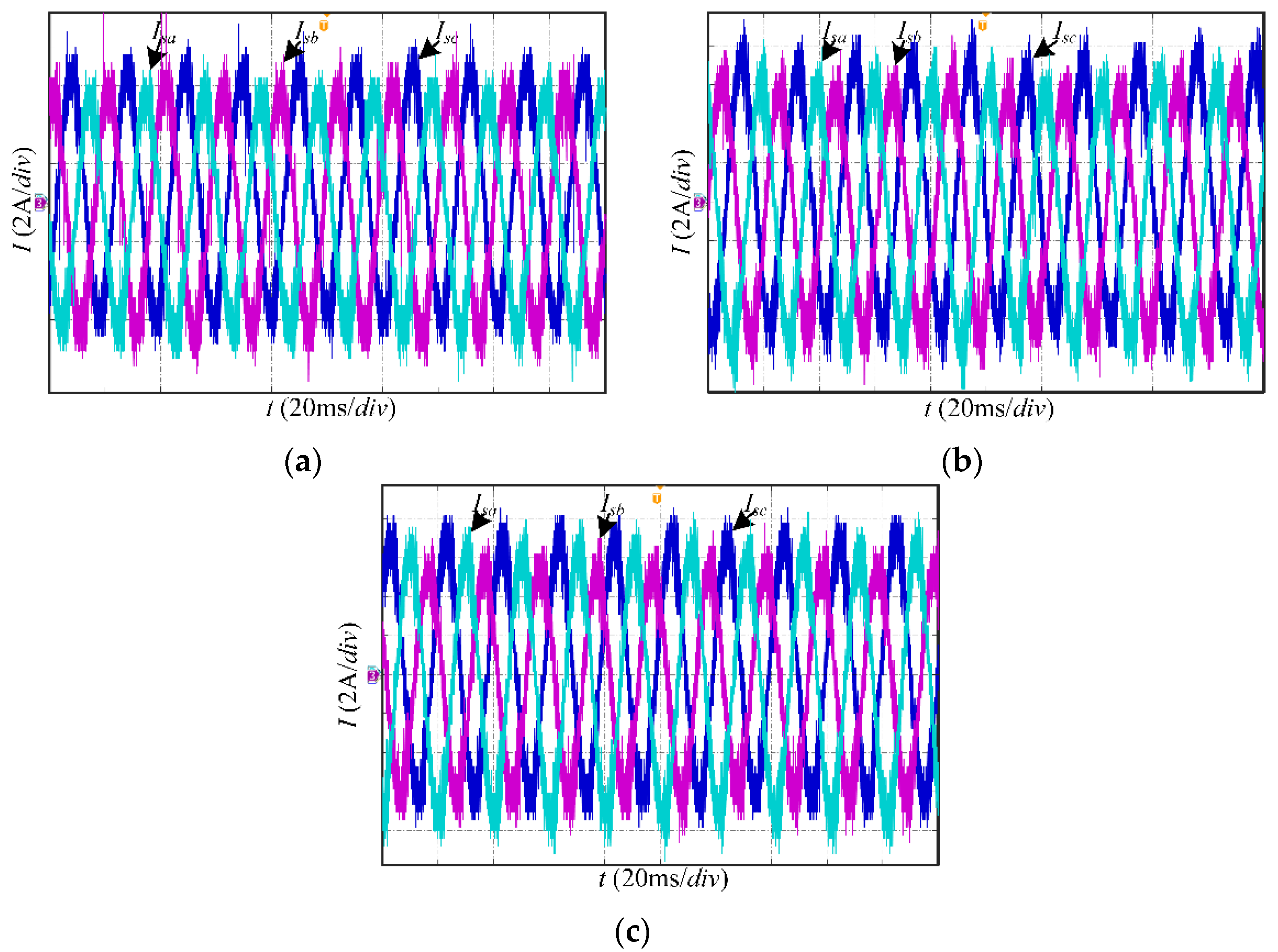
The proposed diagnosis and prediction method was investigated by the simulation and a series of experiments. The simulation and experimental results were consistent, which verifies the correctness and effectiveness of the proposed method.

Notably, the SISCF leads to the asymmetry of stator impedance, which is the cause of the negative sequence component in the stator currents. This study uses the negative sequence current as the object to identify this stator asymmetry fault. Some other im-pedance asymmetry faults inside or outside the stator may cause similar results, such as phase-to-phase short circuit fault.

References

1. Lee, S.B.; Tallam, R.M.; Habetler, T.G. A robust, on-line turn-fault detection technique for induction machines based on monitoring the sequence component impedance matrix. IEEE Trans. Power Electron. 2003, 18, 865–872. [Google Scholar]
2. Bakhri, S.; Ertugrul, N.; Soong, W.L. Negative sequence current compensation for stator shorted turn detection in induction motors. In Proceedings of the IECON 2012-38th Annual Conference on IEEE Industrial Electronics Society, Montreal, QC, Canada, 25–28 October 2012; pp. 1921–1926. [Google Scholar]
3. Kim, K. Simple Online Fault Detecting Scheme for Short-Circuited Turn in a PMSM Through Current Harmonic Monitoring. IEEE Trans. Ind. Electron. 2011, 58, 2565–2568. [Google Scholar] [CrossRef]
4. Radecki, A.; Dębowski, A.; Wójcik, M.; Lipnicki, P. Evaluation of a diagnostic information on common electrical faults contained in signals of an inverter-fed AC IM drive with current-oriented control. In Proceedings of the 2016 10th International Conference on Compatibility, Power Electronics and Power Engineering (CPE-POWERENG), Bydgoszcz, Poland, 29 June–1 July 2016; pp. 286–291. [Google Scholar]
5. Malekpour, M.; Phung, B.T.; Ambikairajah, E. Online technique for insulation assessment of induction motor stator windings under different load conditions. IEEE Trans. Dielectr. Electr. Insul. 2017, 24, 349–358. [Google Scholar] [CrossRef]
6. Nguyen, V.; Wang, D.; Seshadrinath, J.; Ukil, A.; Krishna, M.S.; Nadarajan, S.; Vaiyapuri, V. A Method for Incipient Interturn Fault Detection and Severity Estimation of Induction Motors Under Inherent Asymmetry and Voltage Imbalance. IEEE Trans. Transport. Electrif. 2017, 3, 703–715. [Google Scholar] [CrossRef]
7. Wang, B.; Hu, J.; Wang, G.; Hua, W. A Novel Stator Turn Fault Detection Technique by Using Equivalent High Frequency Impedance. IEEE Access 2020, 8, 130540–130550. [Google Scholar] [CrossRef]
8. Sun, Y.; Yu, X.; Wei, K.; Huang, Z.; Wang, X. A new type of search coil for detecting inter-turn faults in synchronous machines. Proc. CSEE 2014, 34, 917–924. [Google Scholar]
9. Surya, G.N.; Khan, Z.J.; Ballal, M.S.; Suryawanshi, H.M. A Simplified Frequency-Domain Detection of Stator Turn Fault in Squirrel-Cage Induction Motors Using an Observer Coil Technique. IEEE Trans. Ind. Electron. 2017, 64, 1495–1506. [Google Scholar] [CrossRef]
10. Mirzaeva, G.; Saad, K.I. Advanced Diagnosis of Stator Turn-to-Turn Faults and Static Eccentricity in Induction Motors Based on Internal Flux Measurement. IEEE Trans. Ind. Appl. 2018, 54, 3961–3970. [Google Scholar] [CrossRef]
11. Tomczyk, M.; Mielnik, R.; Plichta, A.; Gołdasz, I.; Sułowicz, M. Application of Genetic Algorithm for Inter-Turn Short Circuit Detection in Stator Winding of Induction Motor. Energies 2021, 14, 8523. [Google Scholar] [CrossRef]
12. Zaman, S.M.K.; Liang, X. An Effective Induction Motor Fault Diagnosis Approach Using Graph-Based Semi-Supervised Learning. IEEE Access 2021, 9, 7471–7482. [Google Scholar] [CrossRef]
13. Skowron, M.; Orlowska-Kowalska, T.; Wolkiewicz, M.; Kowalski, C.T. Convolutional Neural Network-Based Stator Current Data-Driven Incipient Stator Fault Diagnosis of Inverter-Fed Induction Motor. Energies 2020, 13, 1475. [Google Scholar] [CrossRef] [Green Version]
14. Jaksch, I. Measuring and evaluating methods for on-line induction motor diagnosis. In Proceedings of the Fifth International Conference on Power Electronics and Drive Systems, Singapore, 17–20 November 2003; pp. 308–312. [Google Scholar]
15. Fonseca, D.S.B.; Santos, C.M.C.; Cardoso, A.J.M. Stator Faults Modeling and Diagnostics of Line-Start Permanent Magnet Synchronous Motors. IEEE Trans. Ind. Appl. 2020, 56, 2590–2599. [Google Scholar] [CrossRef]
16. Cruz, S.M.A.; Cardoso, A.J.M. Stator winding fault diagnosis in three-phase synchronous and asynchronous motors, by the extended Park’s vector approach. IEEE Trans. Ind. Appl. 2001, 37, 1227–1233. [Google Scholar] [CrossRef]
17. Vilhekar, T.G.; Ballal, M.S.; Suryawanshi, H.M. Application of Multiple Parks Vector Approach for Detection of Multiple Faults in Induction Motors. J. Power Electron. 2017, 17, 972–982. [Google Scholar]
18. Spyropoulos, D.V.; Mitronikas, E.D. Induction motor stator fault diagnosis technique using Park vector approach and complex wavelets. In Proceedings of the 2012 XXth International Conference on Electrical Machines, Marseille, France, 2–5 September 2012; pp. 1730–1734. [Google Scholar]
19. Cardoso, A.J.M.; Cruz, S.M.A.; Fonseca, D.S.B. Inter-turn stator winding fault diagnosis in three-phase induction motors, by Park's vector approach. IEEE Trans. Energy Convers. 1999, 14, 595–598. [Google Scholar] [CrossRef]
20. Yan, B.; Wang, B.; Li, Y. Optimal ellipse fitting method based on least square principle. J. Beijing Univ. Aeronaut. Astronaut. 2008, 34, 295–298. [Google Scholar]
21. Zhu, S.; Liu, J. Improved fast algorithm for elliptic fitting based on least square method. Ship Electron. Eng. 2022, 42, 33–35. [Google Scholar]
22. Ding, B. Research on Internal Fault Analysis and Detection Method of Induction Motor. Master’s Thesis, Shandong University, Jinan, China, 2006. [Google Scholar]
Figure 1. Schematic diagram of stator interturn short-circuit fault.
Energies 15 03759 g001
Figure 2. The rotating magnetic field distribution of stator and rotor before and after motor stator failure: (a) healthy motor. (b) Motor with stator interturn short-circuit fault.
Energies 15 03759 g002
Figure 3. Ellipse fitting of Park vector trajectory when motor frequency and load fluctuate: (a) frequency decreases. (b) Frequency increases.
Energies 15 03759 g003
Figure 4. Flow chart of diagnosis and prediction method of stator interturn short-circuit fault.
Energies 15 03759 g004
Figure 5. Main circuit topology diagram of the traction motor.
Energies 15 03759 g005
Figure 6. Stator current of the motor at 30% TN: (a) healthy condition. (b) B, C phase in series with 1 Ω resistors. (c) B, C phase in series with 2 Ω resistors.
Energies 15 03759 g006
Figure 7. Simulation diagram of Park vector trajectory and its fitted ellipse: (a) healthy condition at 30% TN. (b) B and C phase in series with 1 Ω resistors at 30% TN. (c) B and C phase in series with 2 Ω resistors at 30% TN. (d) Healthy condition at 70% TN. (e) B and C phase in series with 1 Ω resistors at 70% TN. (f) B and C phase in series with 2 Ω resistors at 70% TN.
Energies 15 03759 g007aEnergies 15 03759 g007b
Figure 8. Motor negative sequence current and its fitting curve.
Energies 15 03759 g008
Figure 9. Park vector trajectory ellipse long axis tilt angle of simulation data.
Energies 15 03759 g009
Figure 10. Motor negative sequence currents and fitting curves: (a) The motor operates at 10 Hz. (b) The motor operates at 30 Hz.
Energies 15 03759 g010
Figure 11. Park vector trajectory ellipse long axis tilt angle of simulation data: (a) The motor operates at 10 Hz. (b) The motor operates at 30 Hz.
Energies 15 03759 g011
Figure 12. The physical picture of the experimental hardware platform: (a) controller and inverter. (b) Tested motor and load motor.
Energies 15 03759 g012
Figure 13. Stator three-phase currents at 30% TN: (a) healthy condition. (b) B, C phase in series with 1 Ω resistors. (c) B, C phase in series with 2 Ω resistors.
Energies 15 03759 g013
Figure 14. Experimental diagram of Park vector trajectory and its fitted ellipse: (a) healthy condition at 30% TN. (b) B and C phases in series with 1 Ω resistors at 30% TN. (c) B and C phases in series with 2 Ω resistors at 30% TN. (d) Healthy condition at 70% TN. (e) B and C phases in series with 1 Ω resistors at 70% TN. (f) B and C phases in series with 2 Ω resistors at 70% TN.
Energies 15 03759 g014
Figure 15. Motor negative sequence currents and fitting curves.
Energies 15 03759 g015
Figure 16. Park vector trajectory ellipse long axis tilt angle of experimental data.
Energies 15 03759 g016