Abstract
Aiming to solve the problem that the residual life of defective elbows is difficult to predict and the prediction accuracy of a traditional extreme learning machine (ELM) is unsatisfactory, a genetic algorithm optimization neural network extreme learning machine method (GA-ELM) that can effectively predict erosion rate and residual life is proposed. In this method, the input weight and hidden layer node threshold of the hidden layer node is mapped to GA, and the input weight and threshold of the ELM network error is selected by GA, which improves the generalization performance of the ELM. Firstly, the effects of solid particle velocity, particle size, and mass flow rate on the erosion of elbow are studied, and the erosion rates under the conditions of point erosion defect, groove defect, and double groove erosion defect are calculated. On this basis, the optimized GA-ELM network model is used to predict the residual life of the pipelines and then compared with the traditional ELM network model. The results show that the maximum erosion rate of defect free elbow is linearly correlated with solid particle velocity, particle size, and mass flow rate; The maximum erosion rate of defective bend is higher than that of nondefective bends, and the maximum erosion rate of defective bend is linearly related to mass flow rate, but nonlinear to solid particle flow rate and particle size; the GA-ELM model can effectively predict the erosion residual life of a defective elbow. The prediction accuracy and generalization ability of the GA-ELM model are better than those of the traditional ELM model.
1. Introduction
Submarine pipelines play an important part in offshore oil and gas development and transportation. Simultaneously they are currently the safest and most economical way of marine oil and gas transportation; they are also known as the lifeline of offshore oil and gas transportation. Compared with land pipelines, submarine pipelines have to be in a harsh and changeable marine environment for a long time. Oil and gas leakage is often caused by failure and damage caused by various uncontrollable factors [1]. Oil and gas leakage from submarine pipelines brings huge economic losses to the oil industry and natural industry. At the same time, the damage to the marine ecological environment is immeasurable. With the rapid growth of operating time and the total scale of China’s oil and gas pipelines, a series of oil and gas leakage accidents have followed. In 2002 alone, there were four submarine pipelines damage accidents reported by the Offshore Oil Corporation. The most affected organisms in oil spill accidents of submarine oil pipelines are the benthos at the ocean bottom. Oil droplets will adhere to the particles suspended in the ocean and sink to the seabed. These toxic substances flow along the bottom, polluting the bottom of the seabed and affecting benthic organisms. In severe cases, it will cause complete destruction of benthic ecosystems and cause invertebrates to die. The change of the community gradually formed a benthic ecological structure dominated by oil-tolerant species [2].
There are many reasons for submarine oil leakage, among which pipelines fatigue caused by erosion is one of the main reasons for leakage. In recent years, erosion fatigue has become one of the hot research directions of scholars. Scholars have used experimental methods to verify the erosion model at low concentrations [3,4,5,6,7]. Carlos used numerical methods to study the effect of different sand concentrations on elbow erosion. In order to evaluate the quality of numerical predictions of erosion rates, experimental data were used to validate erosion and recovery models at low concentrations [8]. Combining the working conditions of oil and gas wells, An Jie uses the method of mutual verification between simulation and experiment, and deeply analyzes the stress of a single particle in the pipelines [9]. The pipe-flow solid–liquid two-phase flow erosion experimental device developed by Qin Long, which has obtained the conclusion that the erosion rate of sand-carrying fracturing fluid on P110 material increases with the increase in flow rate [10]. Ou Guofu analyzed the mechanism of pipelines erosion damage under the interaction of corrosion and fluid flow. The ANSYS finite element analysis software is used to establish a fluid–structure interaction mathematical model to determine the dangerous area and failure trend of the elbow erosion damage [11]. Zhang Yiwei derived the coiled tubing residual life model and predicted the residual life [12]. Sun Baocai used SVR to predict the residual strength of oil and gas pipelines [13]. Pan Li predicted the corrosion life of non-damaged T-shaped tee pipes, and the average prediction accuracy was 86.1% [14]. Most of the existing papers focus on the analysis of the residual life of the complete pipeline, and there are few studies on the residual life of the defective pipeline. In engineering practice, especially in the middle and later stages of use, pipelines will inevitably have defects, so the research on the residual life of pipelines with defects has more practical significance.
Therefore, this paper comprehensively considers the erosion fatigue of elbows in engineering practice. The erosion rates of defect-free, point erosion defect, single-groove erosion defect, and double-groove erosion defect elbows under different particle flow rates, particle sizes, and mass flow rates were calculated. Then particle size and mass flow rate were calculated as well., This study establishes a pipeline life prediction model based on ELM and GA-ELM and will help to make up for the deficiencies of existing research.
2. Erosion Model of Pipelines in Actual Condition
Particle erosion in pipelines is an important branch of flow assurance topics [15]. In the process of oil and gas production, although is the flow is filtered, the particulate matter will still exist in the oil and gas. After long-term collision with pipelines components such as the inner wall of the pipelines, elbows, etc., it will cause erosion damage to the pipelines system, resulting in dangerous accidents and huge economic losses. Pipelines particle erosion is a very complex process, which is related to many factors such as particle impact velocity of impurity particles in the pipelines, particle physical properties (such as particle size), and particle mass flow rate [16]. Among them, the main reasons for the erosion damage of components are the sudden change of the oil and gas flow direction during the production process or the particle collision caused by the flow restriction [17]. The elbow is a common component in the subsea oil transportation system. When the crude oil flows through the elbow, the impurity particles entrained by it will deviate from the original flow direction and hit the wall of the pipelines to cause erosion damage.
2.1. Governing Equations for the Continuous Phase
Ignoring the effect of temperature on the physical properties of the gas, and considering the gas as an incompressible fluid, the steady-state simulation method is used to simulate the flow field, and the corresponding control equation is:
In Equation (1), is the density; , , and are the component of the velocity vector in the , , directions.
2.2. Predictive Model for Erosion Wear
Oka of Hiroshima University proposed a new particle erosion model based on a large number of particle erosion target experiments. Compared with other traditional models, Oka takes more consideration of erosion wear factors [18], including Vickers number of pipe material (characterizing material hardness), relative velocity, particle diameter, etc.
In Equations (2)–(4), is the corrosion rate, ; is the corrosion impact angle-dependent resistance, ; is the reference wear rate, ; is the Vickers value characterizing the hardness of the wear material; is the collision velocity when the particles collide, ; coefficient: , , , , , , , and .
The turbulent flow is an RNG based on the Boussinesq assumption, the model is strictly derived based on the renormalization group theory, and the specific expression is as follows:
In Equations (5) and (6), effective viscosity ; and are the turbulent kinetic energy; ; is the turbulent diffusion term; is the turbulent kinetic energy; , , and coefficient of turbulent viscosity , additional items:
In Equation (7), , is the strain rate tensor norm; constant , .
The Oka wear model can be transformed into a general formula for wear calculation that is convenient for CFD calculations:
In Equation (8), is the erosion wear rate, ; is the mass flow rate of particles that collide, ; is a function related to particle properties; is the expression of wear amount and collision angle; is the collision velocity when the particles collide, ; is an empirical coefficient describing the contribution of speed to wear; is the discrete element area at the time of collision, .
2.3. Parameters of the Model
The inner diameter of the pipelines of the model established in this section: 0.2 m, and the total height of the pipelines: 11.5 m. The internal fluid is oil and gas, the flow rate is 10 m/s, the particle size is 2.5 × 10⁻⁵ m, and the mass flow rate is 28.33 kg/s. The particles are uniformly released in the pipelines, as shown in Figure 1 for the established pipelines model.
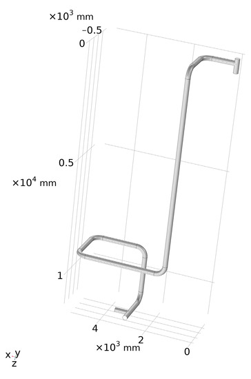
Figure 1.
Pipelines model.
2.4. Mesh Division
Structural meshes are easy to achieve regional boundary fitting, so the straight pipe part of this paper adopts a hexahedral structure mesh, while the elbow, tee, blind tee, and other parts are divided by a tetrahedral mesh with strong adaptability. Local densification is performed at the corresponding elbow. The maximum element of the mesh: 45.8 mm; the minimum element: 0.705 mm; the maximum element growth rate: 1.05; and the total number of meshes is 797,659. Five boundary layers are set near the wall of the mesh, which satisfies the y+ distribution between 30 and 300. The schematic diagram of the mesh is shown in Figure 2.
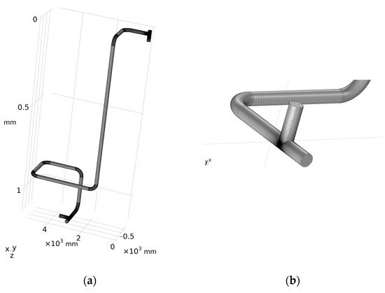
Figure 2.
Mesh schematic diagram. (a) Overall view of the mesh. (b) A zoomed-in view of the mesh.
2.5. Erosion Rate of Pipes
As shown in Figure 3, it can be found that the maximum erosion rate of this model is basically at the elbow, tee, and blind tee, and the maximum erosion rate in this model is 1.96 × 10⁻⁴ kg/(m2·s). Therefore, the next research focus of this paper is the erosion rate of the elbow.
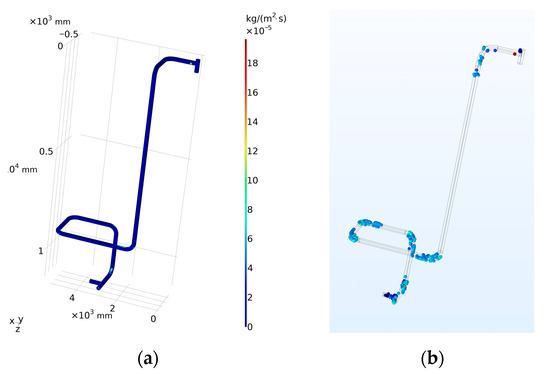
Figure 3.
Schematic diagram of overall erosion rate and particle track of pipelines. (a) Schematic diagram of overall erosion rate. (b) Schematic diagram of overall particle track.
3. Erosion Rate Analysis of 90° Elbow
Studies have shown that in pipeline accidents, about one-third of the accidents are caused by the impact of solid particles entrenched in the fluid and the loss of wall thickness caused by cutting the wall of the pipelines. The effect of the metal wall is stronger, so that the erosion of the elbow is more than 50 times more serious than that of a straight pipe [19]. At present, many experts and scholars have conducted a lot of research on the mechanism of pipelines erosion, which provides technical support for alleviating pipelines erosion and improving the reliability of pipelines transportation. Some scholars use CFD software for simulation analysis. They have carried out effective numerical simulation analysis on the erosion process of gas–solid two-phase flow from various perspectives, and obtained the most critical influencing factors through comparison, such as fluid operating parameters, particle type and size, pipelines structure, etc. Edwards et al. [20] carried out numerical simulation analysis on erosion in elbows and tee pipes, and proposed corresponding mitigation measures. Zeng Li [21], Hu Yuehua [22], Hu Zongwu [23], and others conducted simulation research and analysis on the mechanism and hydraulic characteristics of erosion wear in pipelines, and these studies have reference value for the prevention of erosion wear. In this paper, the numerical simulation method is used to numerically simulate and analyze the flow erosion characteristics of gas–solid two-phase flow on the inner wall of a 90° right-angle elbow, so as to obtain the influence of different parameters on the erosion and wear of the inner wall.
3.1. Model Parameters and Boundary Conditions
According to the test situation of reference [24], a three-dimensional elbow model is established, as shown in Figure 4. Pipe diameter: D = 25.4 mm; wall thickness: h = 12 mm; and the bend–diameter ratio is 1.5. In order to ensure the sufficient development and flow of the incoming flow, this paper establishes an inlet straight pipe section with L1 = 15 D in the upstream direction of the elbow inlet and an outlet straight pipe section with L2 = 10 D in the downstream direction of the outlet. The inside of the pipelines is oil and gas, the gas density is 1.225 kg/m3, and the gas viscosity is 1.79 × 10⁻⁵ Pa·s. The condition at the inlet is the velocity inlet, and the value is 34.1 m/s, the outlet is free flow, and the pipe material is aluminum. The particle size was 182 µm, and the mass flow rate ratio of particles to gas phase was 0.013. The elbow calculation model is shown in Figure 4.
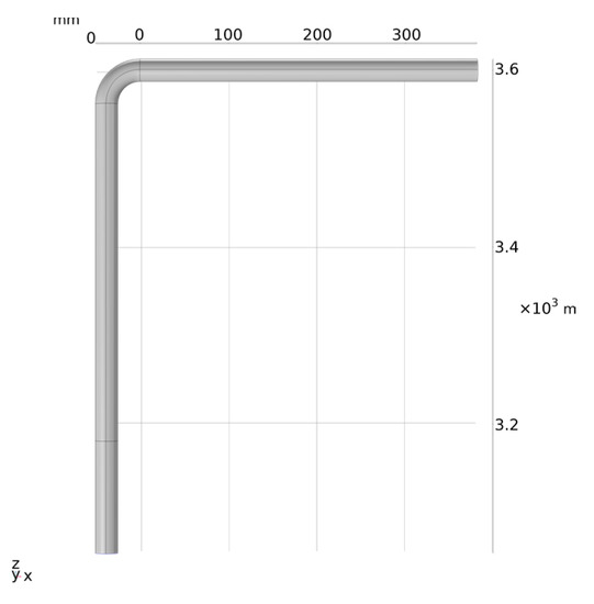
Figure 4.
Calculation model of bending tube.
3.2. Mesh Division and Mesh Independence Verification
The quality and quantity of meshes in CFD directly affect the calculation speed and calculation accuracy. High-quality meshes can not only reduce the calculation memory but also improve the calculation accuracy. The hexahedral structured mesh is used for division. The maximum element of the mesh is 2.41 mm, the minimum element is 0.157 mm, the maximum element growth rate is 1.08, and the total number of meshes is 134,928. Five boundary layers are set up on the near wall of the mesh, and the y+ distribution is between 30 and 300. The result of meshing is shown in Figure 5.
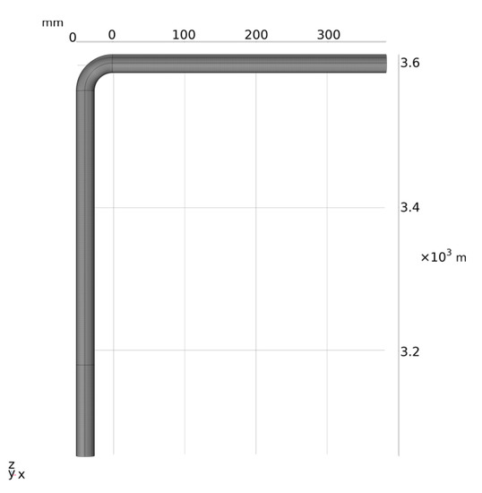
Figure 5.
Mesh division.
At the same time, the density and quality of the mesh directly affect the accuracy of the calculation results, so before the numerical simulation calculation, the model is verified by mesh independence. When the mesh density reaches a certain level, the effect of increasing the number of mesh elements on the calculation results is very small. At this time, it can be considered that the influence of mesh density on the calculation results can be ignored. In this paper, according to the gradient of mesh size, the models with mesh numbers of 11,598, 19,904, 36,715, 134,928, and 264,668 are selected for numerical simulation. The maximum erosion rate curves under different numbers of meshes are shown in Figure 6. It can be seen from Figure 6 that when the number of meshes reaches 134,928, the impact of the number of meshes on the calculation results is small, and the calculation results tend to be stable. At this time, it can be considered that the mesh independence requirement has been met.
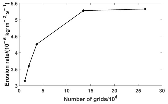
Figure 6.
Mesh-independent validation.
3.3. Validation of Numerical Methods
In order to verify the accuracy of the data, this paper calculates the erosion rate of the elbow under the impact of different numbers of particles. It can be seen from Table 1 that when the number of particles reaches 57,600, the independence of particles is satisfied [24].

Table 1.
Simulation comparison of erosion rate under different particle numbers.
Figure 7 shows the distribution curve of the erosion rate at the outermost side of the elbow, and the test data in the figure are the test results of Mazumder et al. [25]. The outermost erosion rate distribution fits well with the experimental results, indicating that the simulation method and mathematical model used in this paper have good erosion prediction ability.
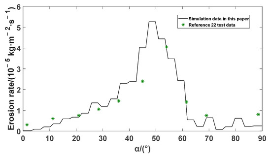
Figure 7.
Comparison diagram of the outermost wear rate distribution of the bends.
3.4. Analysis of Results
The schematic diagram of the erosion rate obtained by the simulation is shown in Figure 8. It can be seen from the figure that the severe erosion area of the elbow is mainly concentrated on the outside of the elbow and is V-shaped. The biggest reason for the above results is that the fluid has a drag force. When the solid particles carried by the fluid move in the pipelines, due to the existence of the elbow, the solid particles impact the inner wall outside the elbow under the action of inertia.
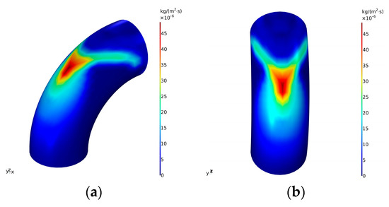
Figure 8.
Schematic diagram of erosion rate distribution at bends. (a) Side view. (b) Front view.
4. Erosion Rate Analysis of Defective Elbow
4.1. Model Parameters
Using the model of 2.1, where the erosion rate is the largest, the wall thickness loss and shape in [25], point defects, single trench defects, and double trench defects with a depth of 200 µm are drawn as shown in Figure 9, Figure 10 and Figure 11.
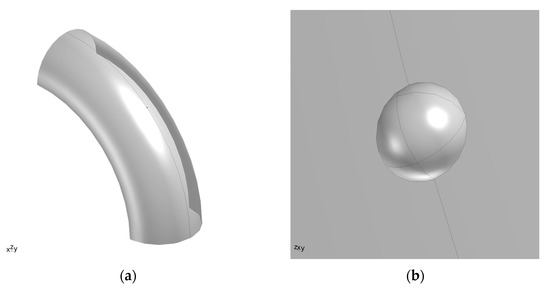
Figure 9.
Point gap position and local amplification drawing at the bend. (a) Point gap position. (b) Local amplification drawing.
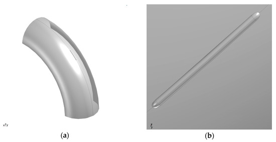
Figure 10.
Position and local amplification drawing of the trench gap at the bend. (a) Trench gap position. (b) Local amplification drawing.
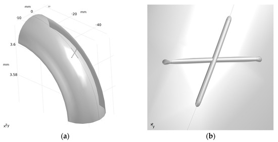
Figure 11.
Position and local amplification drawing of the double trench gap at the bend. (a) Double trench gap position. (b) Local amplification drawing.
4.2. Analysis of Simulation Results
The inlet flow rate is 34.1 m/s, the particle size is 182 µm, and the mass flow rate ratio of particles to gas phase is 0.013. The schematic diagram of the erosion rate obtained by the simulation is shown in Figure 12, Figure 13 and Figure 14.
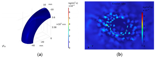
Figure 12.
Erosion rate and local amplification diagram of the point gap at the bend. (a) Schematic diagram of point defect erosion rate. (b) Local amplification drawing.
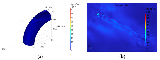
Figure 13.
Erosion rate and local amplification diagram of the trench gap at the bend. (a) Schematic diagram of trench defect erosion rate. (b) Local amplification drawing.
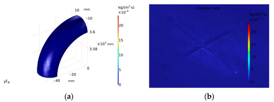
Figure 14.
Erosion rate and local amplification diagram of the double trench gap at the bend. (a) Schematic diagram of double trench defect erosion rate. (b) Local amplification drawing.
By changing the three variables of particle size, flow velocity, and mass flow rate, the erosion rate trends of defect-free, point defects, single-groove defects, and double-groove defects under different boundary conditions are shown in Figure 15, Figure 16, Figure 17, Figure 18, Figure 19 and Figure 20.
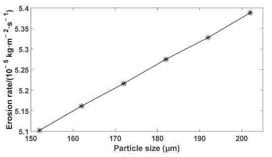
Figure 15.
Particle size is a variable (no gap).
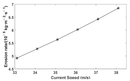
Figure 16.
Flow rate is a variable (no gap).
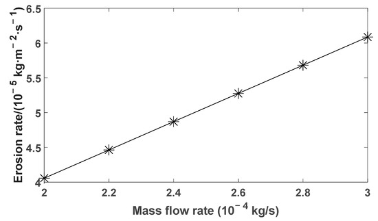
Figure 17.
Mass flow rate is the variable (no gap).
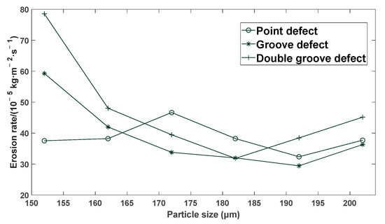
Figure 18.
Particle size is a variable (with a gap).
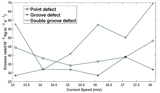
Figure 19.
Flow rate is a variable (with a gap).
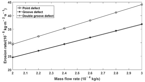
Figure 20.
Mass flow rate as variable (with a gap).
As shown in Figure 15, the maximum erosion rate under different particle sizes was calculated by selecting the conditions that the flow velocity was 34.1 m/s and the gas mass flow rate was 2.6 × 10⁻⁴ kg/s.
As shown in Figure 16, the maximum erosion rate under different flow rates was calculated by selecting the gas mass flow rate of 2.6 × 10⁻⁴ kg/s and the particle size of 182 µm was unchanged.
As shown in Figure 17, the maximum erosion rate under different mass flow rates was calculated by selecting the condition that the flow velocity was 34.1 m/s and the particle size was 182 µm unchanged. It can be seen from the analysis of Figure 15, Figure 16 and Figure 17 that when the pipelines has no defects, the value of the maximum erosion rate is linearly related to the variables such as particle size, flow rate and mass flow rate. As shown in Figure 18, Figure 19 and Figure 20 consistent with the boundary conditions set when there is no defect, the maximum erosion rate under different variable conditions is obtained and the distribution curve is drawn.
It is known from Figure 18 and Figure 19 that the particle size and flow rate under the three defect conditions are all nonlinear with the value of the maximum erosion rate. The maximum erosion rate of double trench defects is generally greater than that of single trench defects.
It can be seen from Figure 20, the values of the mass flow rate under the three defect conditions are linearly related to the value of the maximum erosion rate.
The maximum erosion rate of point defects is generally greater than that of single-groove and double-groove defects. The maximum erosion rates for single and double trench defects are similar. It can be seen that the maximum erosion rate distributed as a variable with mass flow rate is mainly affected by the defect shape and has nothing to do with the number of grooves.
5. Prediction of Erosion Rate and Erosion Life
The prediction of pipelines erosion life is of great significance to the safety and reliability of pipelines [26,27,28]. In this paper, a total of 300 sets of erosion rate and erosion life data for non-defective, point defect, and trench defect elbows are calculated by simulation, of which 250 sets are used as the training set and the remaining 50 sets are used as the test set.
5.1. Extreme Learning Machine
Extreme learning machine (ELM) is a new type of learning algorithm, which is a single-hidden layer feedforward neural network learning algorithm [29]. Compared with the traditional gradient-based learning algorithm, the output weight can be calculated by randomly selecting the input weight and the threshold of the hidden layer nodes, avoiding the problems faced by the traditional learning method. ELM has a fast learning speed and good generalization performance, and its network structure is shown in Figure 21.
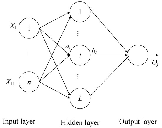
Figure 21.
ELM network structure.
Given the training set , the hidden layer node excitation function is a nonlinear function, including Hardlim function, Sigmoid function, Gaussian function, etc. Among them, the Sigmoid function is the most commonly used, and the number of hidden layer nodes is L.
- (1)
- The randomly selected hidden layer node parameter , i = 1, …, L, ai is the input weight of the ith hidden layer node, and is the threshold of the ith hidden layer node.
- (2)
- Calculate the hidden layer node output matrix .
- (3)
- Calculate the output weight β from the hidden layer to the output layer:
In Equation (10), H↑ is the Moore–Penrose generalized inverse of the hidden layer output matrix H, and T is the target output, namely .
- (4)
- Calculate the output value.
When trained to an error smaller than a preset constant ε, the ELM can approximate these training samples:
- (5)
- Find the error:
Among them, is the input weight and threshold of the hidden layer node, is the actual output value of the jth group of data, and is the output predicted value of the jth group of data. The goal of GA-ELM is to minimize the error . The main idea of this method is: take the initial input weight of ELM and the threshold of hidden layer nodes as the chromosome vector of GA algorithm, and select the most suitable chromosome as the input weight and threshold of ELM prediction data through operations such as selection, crossover, mutation, etc.
5.2. Building a GA-ELM Network Prediction Model
ELM model also has some disadvantages, for example, the input weights and the thresholds of the model are generated randomly, which leads to the lack of adjustment ability of hidden layer neurons. Therefore, genetic algorithm (GA) is selected to find the best weights and thresholds of the model. GA is a method to search the optimal result by imitating the process of chromosome–gene crossover and mutation in the process of biological evolution. The ELM model optimized by GA has both the global optimization ability of GA and the powerful learning capacity of ELM. Therefore, GA–ELM has high accuracy and stability. The flow chart and specific working steps of the algorithm are shown in Figure 22:
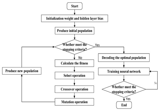
Figure 22.
Algorithm flow chart of GA–ELM model.
- (1)
- Parameter setting. Set the number of neurons of ELM model according to the dimension of input and output data, generate a batch of weights and thresholds randomly; set the maximum evolutionary iterations G, the population size, the crossover probability, the mutation probability, and the generation gap of GA and generate the initial population; and use D to represent the length of individual, where D = (n + 1) L, n represents the input vector dimension and L represents the number of hidden layer nodes.
- (2)
- Calculate the fitness of the population. The root mean square error between the actual output and the expected output is used to measure the merit degree. In each generation of the population, the chromosomes will continue to crossover and mutate to form new populations until restraint conditions are met or the maximum number of iterations is met.
- (3)
- ELM model training, prediction, and verification. Decode the optimal population and obtain the input weights and thresholds. Train the ELM model and then use the test samples to verify the accuracy of the prediction.
5.3. Forecast Results and Analysis
Taking the particle size, flow rate, and mass flow rate of impurity particles as input, and the erosion rate and residual life of elbow as output, respectively, the prediction model of erosion rate and residual life of defective elbow can be obtained by training the three-layer neural network.
This paper takes 250 samples for the training set and 50 samples for the test set. No defect is set to 0, point defect is set to 1, and trench defect is set to 2; some sample data are shown in Table 2.
Table 2.
Sample data.
The safe allowable wall thickness of the pipe wall is h, and the density of aluminum is ρ. According to the erosion rate R, the equation for establishing the erosion life T is shown in Equation (13) [14].
The residual life of the pipelines can be obtained by bringing the parameters into Equation (13), part of the data is listed in Table 2.
Through 50 times, 100 times, 400 times, 600 times, and 1000 times of iterations, the comparison of the prediction accuracy of the elbow is obtained, and the curve of the maximum erosion rate is generated, as shown in Figure 23. It can be seen from Figure 23 that when the number of iterations reaches 600, the impact of the number of iterations on the calculation results is small and the calculation results tend to be stable. At this time, it can be considered that the requirement that the prediction accuracy rate is independent of the number of iterations is met.
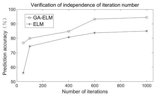
Figure 23.
Number of iterations—independent validation.
Figure 24 and Figure 25 are the comparison charts of the prediction results of the two prediction models. It can be seen from the figure that the accuracy of ELM model in predicting the maximum erosion rate and residual life is 88.378% and 90.58%, while the accuracy of GA-ELM model is 93.679% and 93.547, respectively. The prediction accuracy of GA-ELM model is higher than that of ELM model, which proves that the optimization algorithm can significantly improve the prediction accuracy.
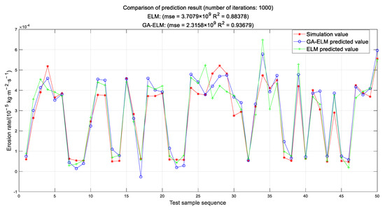
Figure 24.
Comparison of two algorithms for erosion rate prediction.
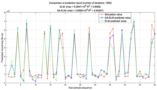
Figure 25.
Comparison of two algorithms for remaining life prediction.
6. Conclusions
This paper takes the 90° right-angle elbow as the research object, uses the method of numerical simulation to model, calculate, and analyze the influence of three main factors of solid particle velocity, particle size, and mass flow rate on the erosion of the elbow with and without defects. Additionally, combined with the algorithm to predict the erosion life. From the present study, the following conclusions were made:
- (1)
- As has been noted, the simulation results of the CFD numerical simulation are in good agreement with the experimental data in the published papers, which verifies that the simulation method and mathematical model can calculate the erosion characteristics of the pipelines well.
- (2)
- In order to study the relationship between particle size, flow rate, mass flow rate, and erosion rate of impurity particles, it is found through simulation calculation that the maximum erosion rate of defect-free elbows is linearly related to the flow rate, particle size and mass flow rate of solid particles. Additionally, the maximum erosion rate of defective elbows is greater than that of defect-free ones; the maximum erosion rate for defective elbows is linearly related to mass flow rate but nonlinearly related to solid particle flow rate and particle size.
- (3)
- For the problem that the erosion rate and residual life of defective pipes cannot be directly obtained, the extreme learning machine GA-ELM model optimized by genetic algorithm is used in this paper to predict the erosion rate and erosion life of defective elbows. The results show that the optimization algorithm compared with the traditional extreme learning machine ELM model, it can effectively improve the prediction accuracy, and provides a theoretical basis for the prediction of erosion rate and residual life of defective elbows in practical engineering applications.
- (4)
- In engineering practice, the particles colliding with the pipe wall will consume a part of the energy, and the pipe will vibrate on the seabed due to the flow of seawater, which will affect the inside of the elbow. In this paper, in order to simplify the calculation, all the above conditions are ignored, and the neglected condition will be a major issue for future research. In conclusion, there are limitations in the simulation research results at this stage, and in-depth research will be carried out in combination with experiments in the future.
Author Contributions
Conceptualization, C.S. and Y.L. (Yuechan Liu); methodology, C.S.; software, Y.L. (Yuelin Li); validation, C.S. and Y.L. (Yuechan Liu); formal analysis, Q.W. and Y.L. (Yuelin Li); investigation, C.S.; data curation, Q.W. and Y.L. (Yuelin Li); writing—original draft preparation, Q.W.; writing—review and editing, Y.L. (Yuechan Liu); supervision, C.S.; project administration, C.S. All authors have read and agreed to the published version of the manuscript.
Funding
This research was funded by the National Natural Science Foundation of China (11704090), University Nursing Program for Young Scholars with Creative Talents in Heilongjiang Province (UNPYSCT-2018207), and the project of Nature Scientific Foundation of Heilongjiang Province (LH2020A016).
Institutional Review Board Statement
Not applicable.
Informed Consent Statement
Not applicable.
Data Availability Statement
Data is available in the paper.
Conflicts of Interest
The authors declare no conflict of interest.
References
- Zhao, J. Risk assessment of oil and gas submarine pipeline. Oil Gas Storage Transp. 2007, 11, 5–8 + 62 + 65. (In Chinese) [Google Scholar]
- Zeng, J.; Xu, X.; Shou, L.; Liao, Y.; Chen, Q.; Zheng, P. Ecological risk and Preventive Countermeasures of oil spill from submarine oil pipeline. Ocean Dev. Manag. 2007, 3, 120–123. (In Chinese) [Google Scholar]
- Li, J. Experimental and Numerical Simulation Study on Erosion Wear of Petrochemical Pipeline; China University of Petroleum: Beijing, China, 2017. (In Chinese) [Google Scholar]
- Cao, X.; Li, X.; Fan, Y.; Wang, K. Research progress of solid particle erosion theory and experiment. Oil Gas Storage Transp. 2019, 38, 251–257. (In Chinese) [Google Scholar]
- Wen, X. Erosion Analysis and Experimental Study of Bend Section of Submarine Pipeline; China University of Petroleum: Beijing, China, 2015. (In Chinese) [Google Scholar]
- Zhang, M. Study on Erosion Mechanism and Flow Field Numerical Simulation of Multiphase Mixed Transmission Pipeline; Northeast Petroleum University: Daqing, China, 2021. (In Chinese) [Google Scholar]
- Parancheerivilakkathil, M.S.; Parapurath, S.; Ainane, S.; Yap, Y.F.; Rostron, P. Flow Velocity and Sand Loading Effect on Erosion–Corrosion during Liquid-Solid Impingement on Mild Steel. Appl. Sci. 2022, 12, 2530. [Google Scholar] [CrossRef]
- Varaksin, A.Y. Collision of Particles and Droplets in Turbulent Two-Phase Flows. High Temp. 2019, 4, 555–572. [Google Scholar] [CrossRef]
- An, J. Numerical Simulation of Particle Erosion of Oil and Gas Well String; Changjiang University: Jingzhou, China, 2014. (In Chinese) [Google Scholar]
- Qin, L. Research and Development of Tubular Liquid-Solid Two-Phase Flow Erosion Experimental Device; Xi’an University of Petroleum: Xi’an, China, 2016. (In Chinese) [Google Scholar]
- Ou, G.; Xu, G.; Zhu, Z.; Yang, J.; Wang, Y. Fluid structure coupling mechanism and numerical simulation of elbow erosion failure. J. Mech. Eng. 2009, 11, 7. (In Chinese) [Google Scholar]
- Zhang, Y. Study on Erosion Wear and Residual Life of Coiled Tubing; Southwest Petroleum University: Chengdu, China, 2017. (In Chinese) [Google Scholar]
- Sun, B.; Zhu, C.; Ling, X. Research on residual strength of pipeline with defects based on SVR. China’s Saf. Prod. Sci. Technol. 2022, 18, 172–176. (In Chinese) [Google Scholar]
- Pan, L. Failure Analysis and Life Prediction of T-Type Tee for Fracturing Manifold; Yangtze University: Jinzhou, China, 2019. (In Chinese) [Google Scholar]
- Davalath, J.; Hurtado, M.; Keig, R. Flow Assurance Management for Bijupira and Salema Field Development. In Proceedings of the Offshore Technology Conference, Houston, TX, USA, 6–9 May 2002. [Google Scholar]
- Barton, M.; Kilbride, E.; Qu, G. Executive Erosion in Elbows in Hydrocarbon Production Systems: Review Document, 1st ed.; TÜV NEL Limited: Glasgow, UK, 2014; pp. 8–9. [Google Scholar]
- Wang, S.; Liu, H.; Zhang, R.; Liu, M. Numerical simulation of sand erosion of submarine pipeline and evaluation of erosion formula. Ocean Eng. 2014, 32, 49–59. (In Chinese) [Google Scholar]
- He, Z.; He, J. Numerical simulation of erosion characteristics of particle water two-phase flow in right angle elbow. Sci. Technol. Innov. 2020, 29, 1–4. (In Chinese) [Google Scholar]
- Huang, Y.; Jiang, X.; Shi, Z. Erosion problem of elbow and its prediction and prevention. Oil Refin. Technol. Eng. 2005, 2, 33–36. (In Chinese) [Google Scholar]
- Levin, B.F.; Vecchio, K.S.; Dupont, J.N. Modeling solid-particle erosion of ductile alloys. Metall. Mater. Trans. A 1999, 30, 1763–1774. [Google Scholar] [CrossRef]
- Zeng, L. Erosion Corrosion Mechanism and Hydrodynamic Characteristics of Pipe Elbow; Huazhong University of Science and Technology: Wuhan, China, 2017. (In Chinese) [Google Scholar]
- Hu, Y. Evaluation of Erosion-Corrosion in Tvpical Pipe Fittings via CFD; Zhejiang University: Hangzhou, China, 2012. (In Chinese) [Google Scholar]
- Hu, Z. Study on Erosion and Corrosion Behavior of 90 Degree Horizontal Elbow under Liquid-Solid Two-Phase Flow; China University of Petroleum: Beijing, China, 2016. (In Chinese) [Google Scholar]
- Zhuo, K.; Qiu, Y.; Zhang, Y.; Wu, D. Influence of particle parameters on erosion wear of gas-solid two-phase flow. J. Xi’an Univ. Pet. (Nat. Sci. Ed.) 2020, 35, 100–106. [Google Scholar]
- Mazumder, Q.H.; Shirazi, S.A.; Mclaury, B. Experimental investigation of the location of maximum erosive wear damage in elbows. J. Press. Vessel Technol. 2008, 130, 011303. [Google Scholar] [CrossRef]
- Li, B.; Zeng, M.; Wang, Q. Numerical Simulation of Erosion Wear for Continuous Elbows in Different Directions. Energies 2022, 15, 1901. [Google Scholar] [CrossRef]
- Hong, B.; Li, Y.; Li, X.; Ji, S.; Yu, Y.; Fan, D.; Qian, Y.; Guo, J.; Gong, J. Numerical Simulation of Gas-Solid Two-Phase Erosion for Elbow and Tee Pipe in Gas Field. Energies 2021, 14, 6609. [Google Scholar] [CrossRef]
- Wang, W.; Sun, Y.; Wang, B.; Mei, D. CFD-Based Erosion and Corrosion Modeling of a Pipeline with CO2-Containing Gas–Water Two-Phase Flow. Energies 2022, 15, 1694. [Google Scholar] [CrossRef]
- Lei, L. Research on Building Energy Consumption Forecasting Based on GA-ELM Method; Xi’an University of Architecture and Technology: Xi’an, China, 2020. (In Chinese) [Google Scholar]
Publisher’s Note: MDPI stays neutral with regard to jurisdictional claims in published maps and institutional affiliations. |
© 2022 by the authors. Licensee MDPI, Basel, Switzerland. This article is an open access article distributed under the terms and conditions of the Creative Commons Attribution (CC BY) license (https://creativecommons.org/licenses/by/4.0/).