
Microgrid Assisted Design for Remote Areas


Abstract
:1. Introduction
- A three-stage MILP is proposed for optimal expansion planning and operation of isolated multienergy microgrids considering legacy DGs and ESSs.
- For practical purpose, the available capacity of DGs (except PV) and ESSs is modeled as discrete constants instead of continuous variables. In addition, the commitment status and minimum output of dispatchable DGs are explicitly modeled.
- To represent the electricity and heat flow between generation resources and various electrical, heating and cooling loads in the isolated microgrid, linearized power flow and heat flow constraints are employed in the proposed optimization model.
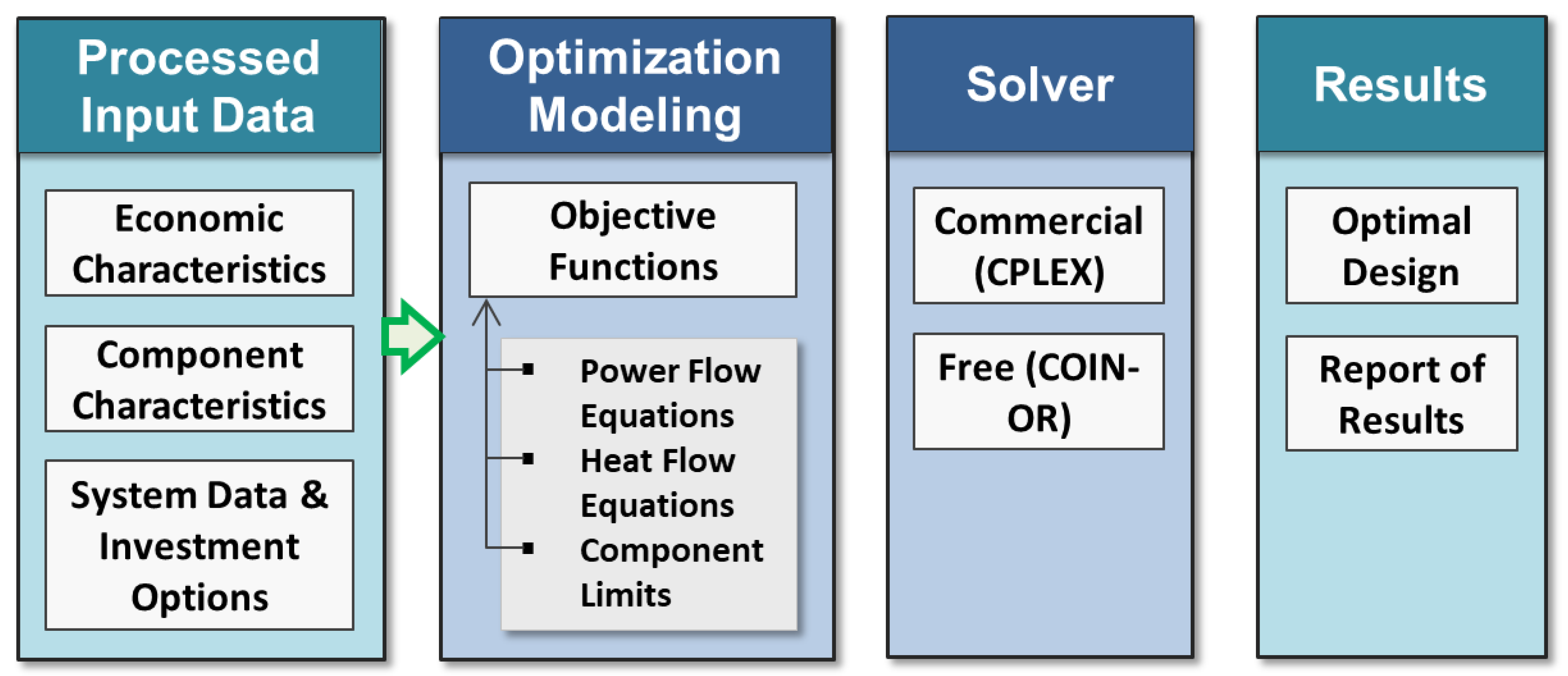
2. Mathematical Formulations
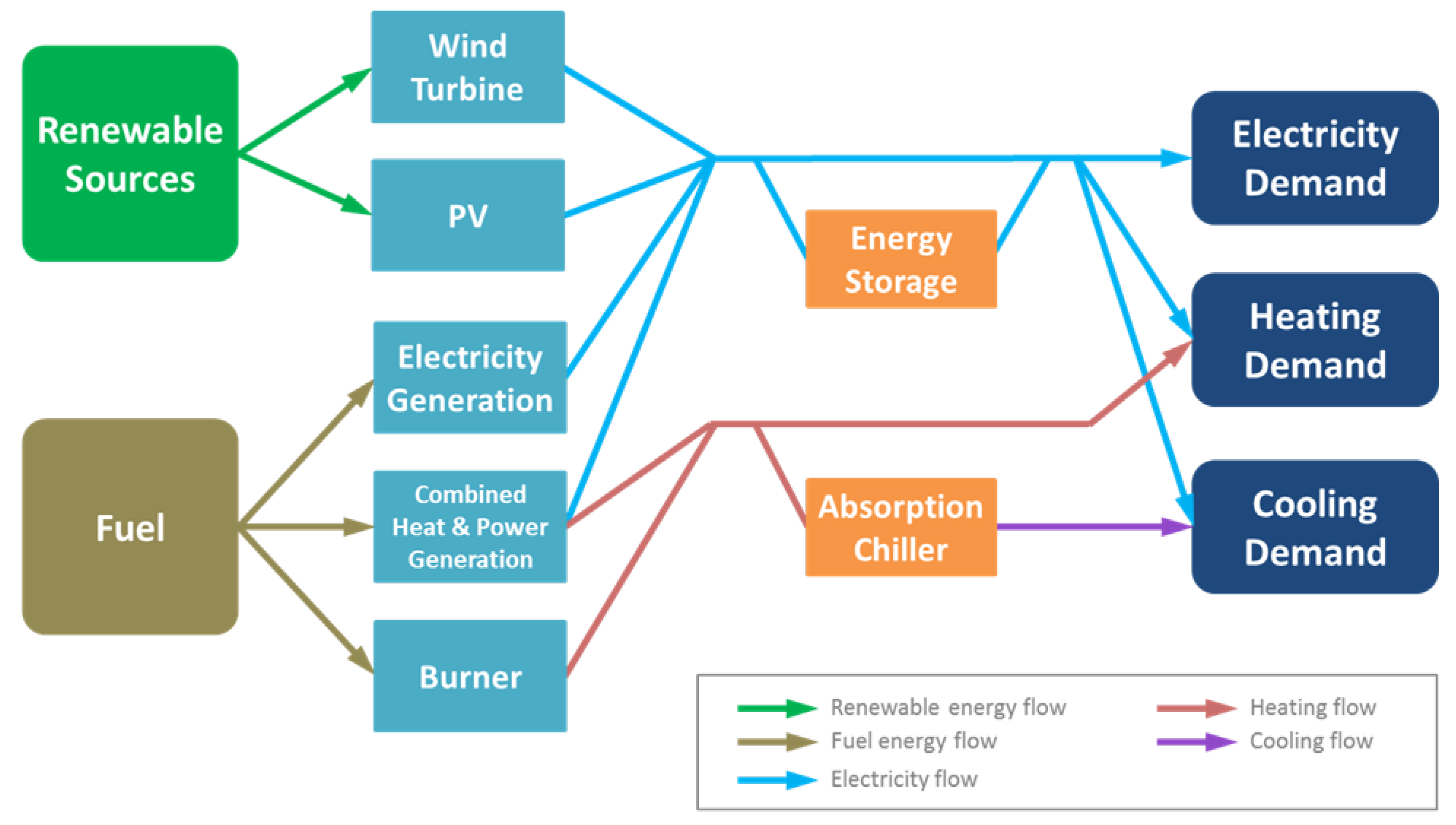
2.1. Microgrid Components
2.2. Objective Function
2.3. Constraints
2.3.1. PV Constraints
2.3.2. Fuel Cell Constraints
2.3.3. Fuel Cell CHP Constraints
2.3.4. Gas Turbine Constraints
2.3.5. Gas Turbine CHP Constraints
2.3.6. ESS Constraints
2.3.7. Network Constraints
2.3.8. Simplification and Linearization
3. Case Studies
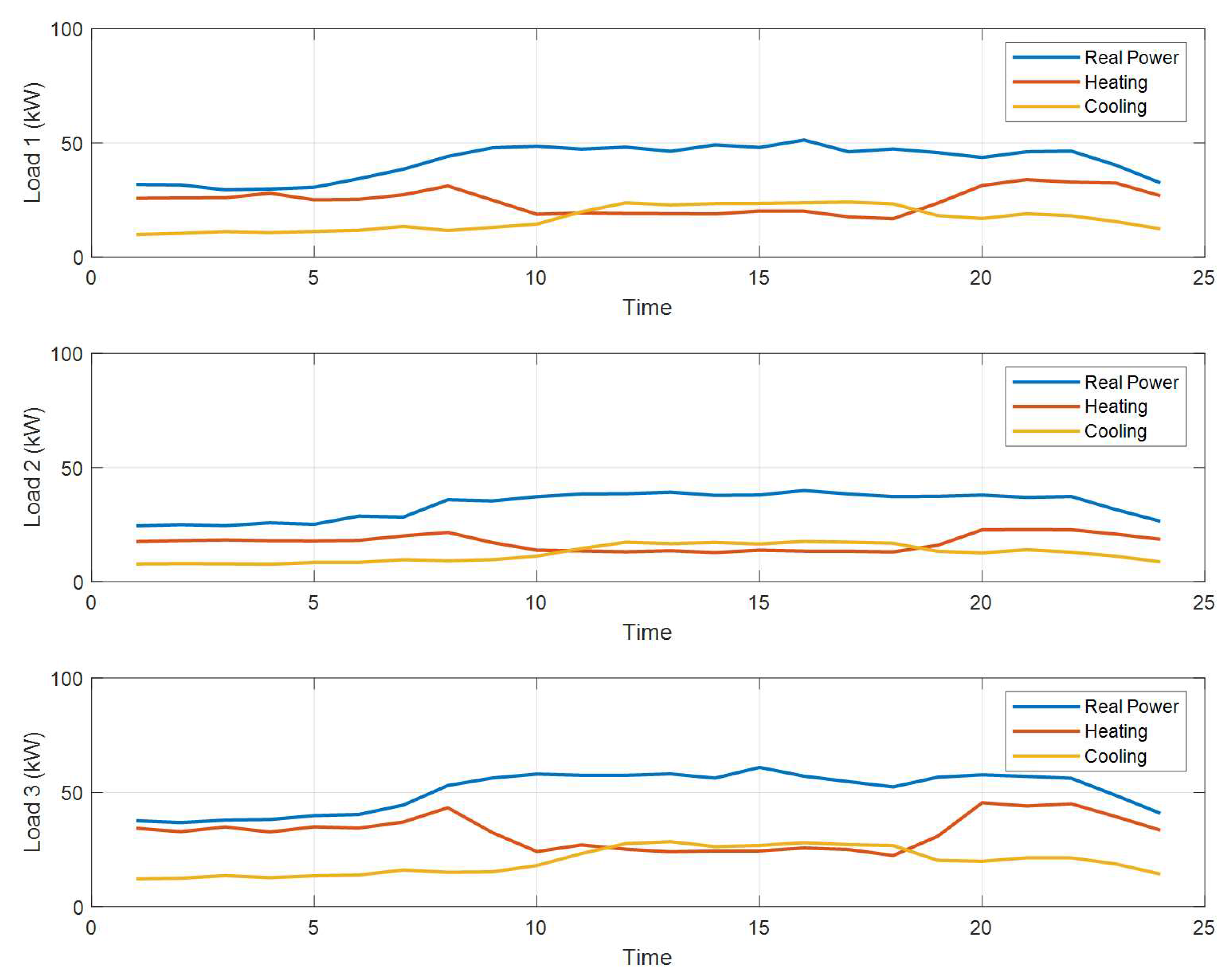
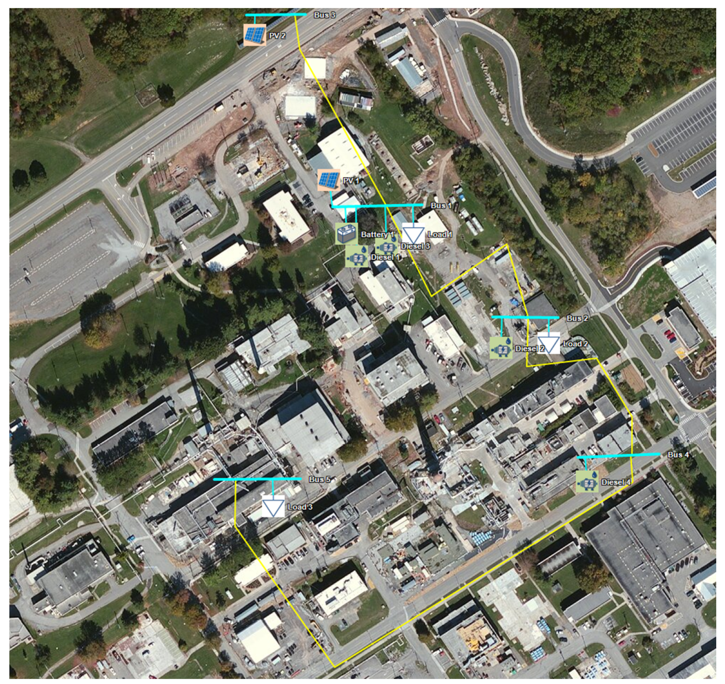
3.1. Test System
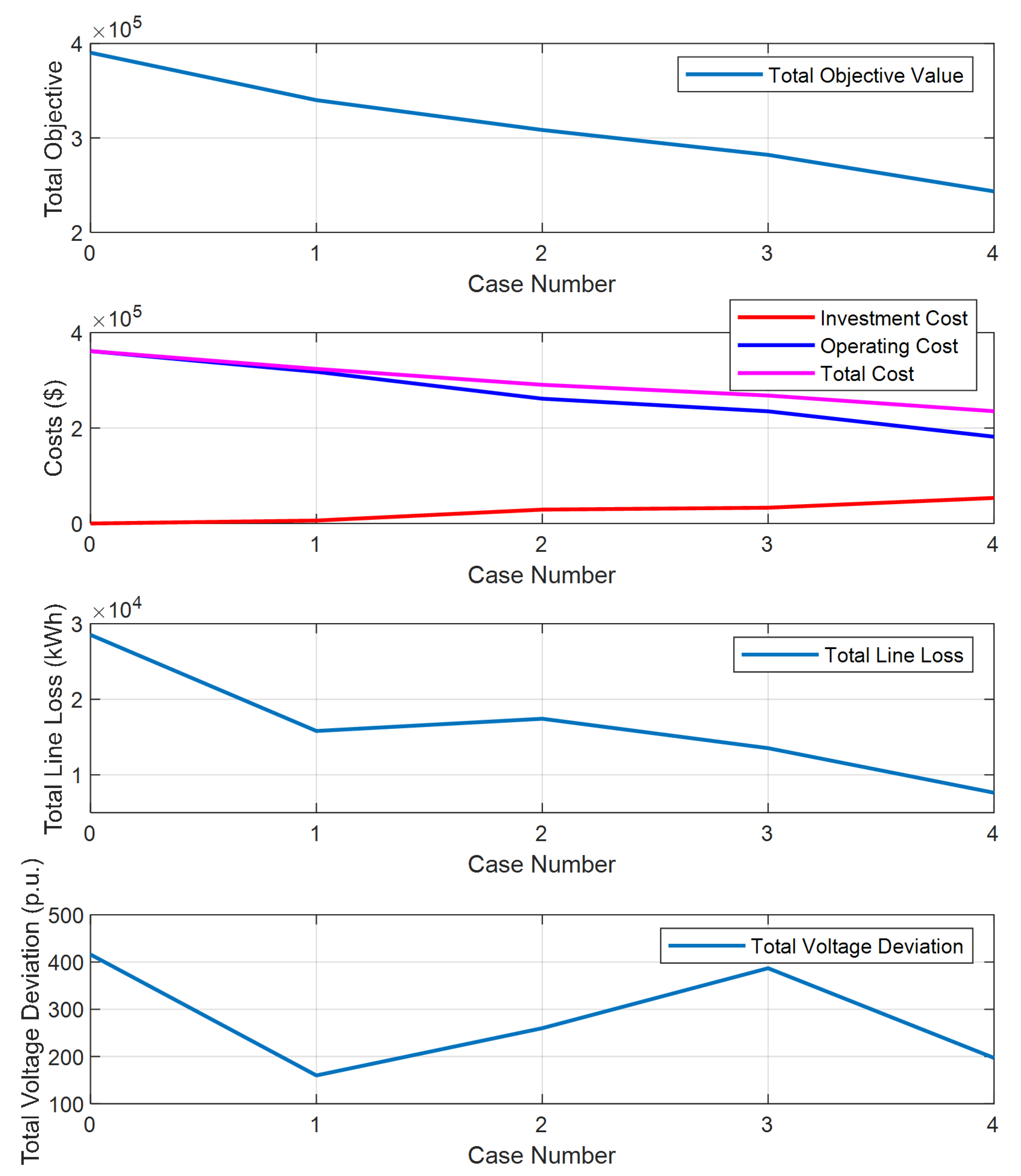
3.2. Results of Case Studies
- Case 0: No investment available;
- Case 1: Only ESS investment available on bus 5;
- Case 2: Only ESS and PV investment available on bus 5;
- Case 3: All technology investment available on bus 5;
- Case 4: All technology investment available on all buses.
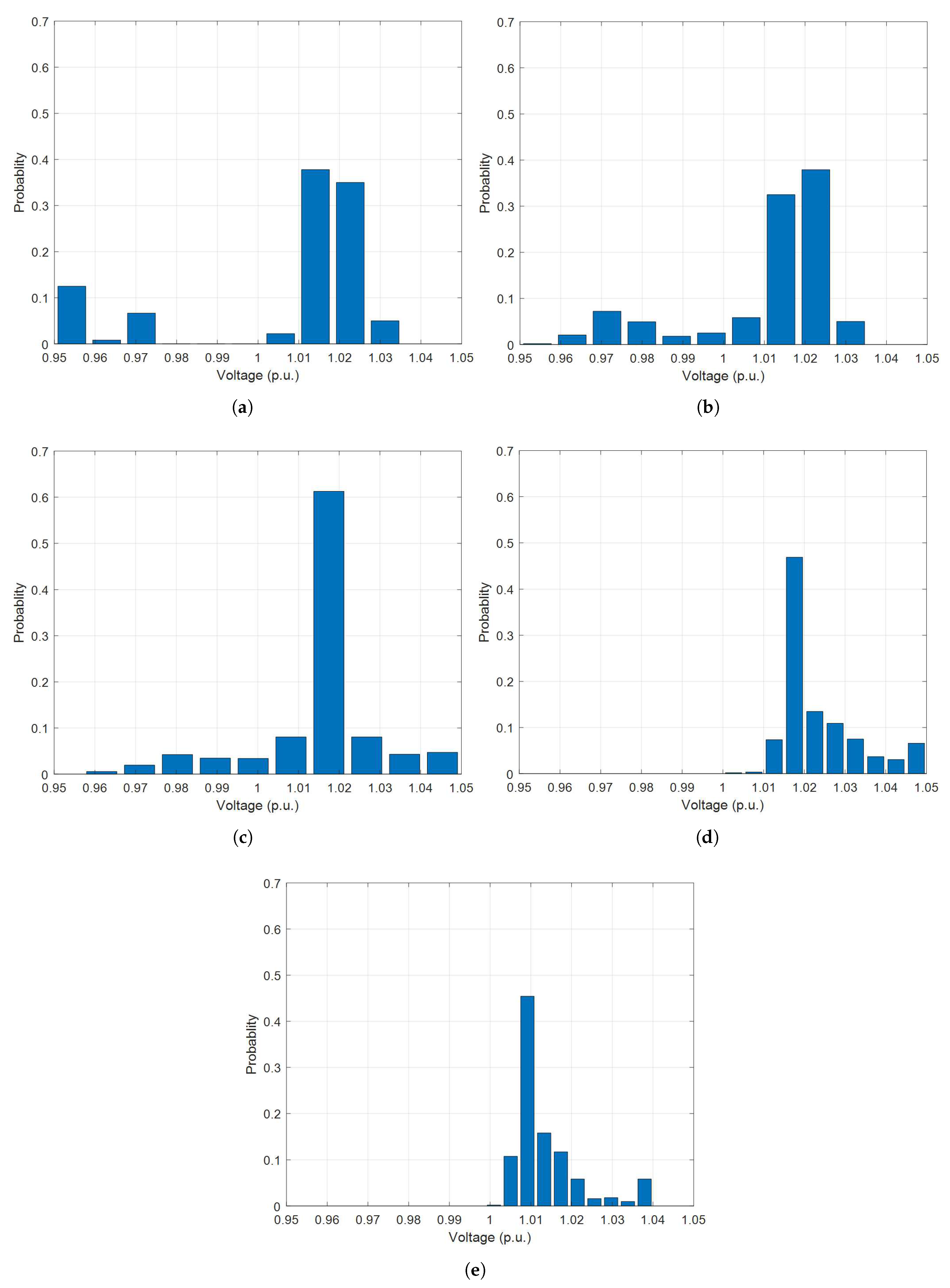
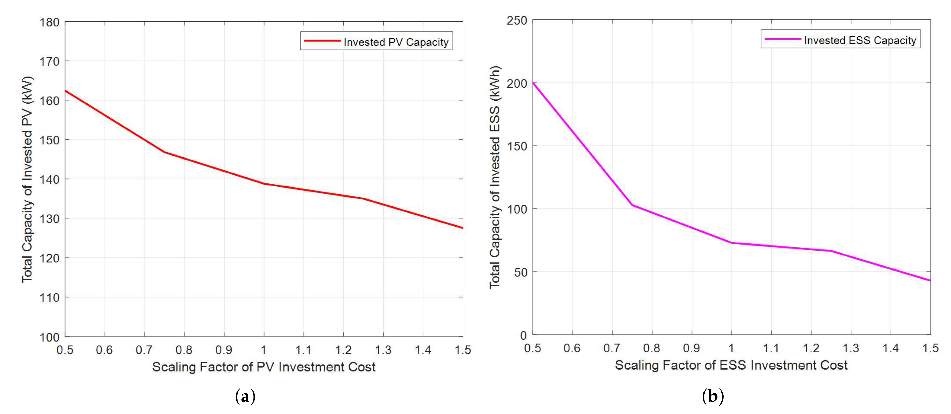
3.3. Sensitivity Analysis
4. Conclusions
- Expanding the current balanced power flow model to practical three-phase unbalanced situation.
- Improving the heat flow model to consider the heating losses of the heat distribution network.
- Enhancing the resilience of power supply under extreme weather events by integrating the reliability and resilience of microgrids into the objective function or constraints.
Author Contributions
Funding
Institutional Review Board Statement
Informed Consent Statement
Data Availability Statement
Acknowledgments
Conflicts of Interest
Nomenclature
| Indices and Numbers | |
| n | Index of buses, running from 1 to |
| j | Index of selections for each technology |
| i | Index of numbers for a specific selection for each technology |
| t | Index of time periods, running from 1 to |
| m | Index of energy blocks offered by DGs, running from 1 to |
| Number of photovoltaics (PV) investment selections and existing PV | |
| Number of fuel cell investment selections and existing fuel cells | |
| Number of candidate units in fuel cell investment selection j | |
| Number of fuel cell combined heat and power (CHP) investment | |
| selections and existing fuel cell CHP | |
| Number of candidate units in fuel cell CHP investment selection j | |
| Number of gas turbine investment selections and existing gas turbines | |
| Number of candidate units in gas turbine investment selection j | |
| Number of gas turbine CHP investment selections and existing gas | |
| turbine CHP | |
| Number of candidate units in gas turbine CHP investment selection j | |
| Number of energy storage system (ESS) investment selections and | |
| existing ESSs | |
| Number of candidate units in ESS investment selection j | |
| Variables | |
| Binary Variables | |
| 1 if fuel cell i of size selection j is invested at bus n and 0 otherwise. | |
| 1 if fuel cell CHP i of size selection j is invested at bus n and 0 otherwise. | |
| 1 if gas turbine i of size selection j is invested at bus n and 0 otherwise. | |
| 1 if gas turbine CHP i of size selection j is invested at bus n and 0 | |
| otherwise. | |
| 1 if ESS i of size selection j is invested at bus n and 0 otherwise. | |
| 1 if fuel cell i of size selection j at bus n is scheduled on during period t | |
| and 0 otherwise. | |
| 1 if fuel cell CHP i of size selection j at bus n is scheduled on during | |
| period t and 0 otherwise. | |
| 1 if gas turbine i of size selection j at bus n is scheduled on during | |
| period t and 0 otherwise. | |
| 1 if gas turbine CHP i of size selection j at bus n is scheduled on during | |
| period t and 0 otherwise. | |
| 1 if ESS i of size selection j at bus n is scheduled charging/discharging | |
| during time t and 0 otherwise. | |
| 1 if existing fuel cell i is scheduled on during period t and 0 otherwise. | |
| 1 if existing fuel cell CHP i is scheduled on during period t and 0 | |
| otherwise. | |
| 1 if existing gas turbine i is scheduled on during period t and 0 | |
| otherwise. | |
| 1 if existing gas turbine CHP i is scheduled on during period t and 0 | |
| otherwise. | |
| 1 if existing diesel generator i is scheduled on during period t and 0 | |
| otherwise. | |
| Continuous Variables | |
| Invested capacity of PV selection i at bus n. | |
| Power of invested PV selection i at bus n during period t. | |
| Power output scheduled from the m-th block of energy offer by fuel cell i | |
| of size selection j at bus n during period t. Limited to . | |
| Power output scheduled from the m-th block of energy offer by fuel cell | |
| CHP i of size selection j at bus n during period t. Limited to . | |
| Power output scheduled from the m-th block of energy offer by gas | |
| turbine i of size selection j at bus n during period t. Limited to . | |
| Power output scheduled from the m-th block of energy offer by gas | |
| turbine CHP i of size selection j at bus n during period t. Limited to | |
| . | |
| Charging/discharging power of ESS i of size selection j at bus n during | |
| period t. Limited to and . | |
| Purchased natural gas for direct heating at bus n during time t. | |
| Real/ reactive power on line f during period t. | |
| Real/reactive power output of fuel cell i of size selection j at bus n during | |
| period t. | |
| Real/reactive power output of fuel cell CHP i of size selection j at bus n | |
| during period t. | |
| Real/reactive power output of gas turbine i of size selection j at bus n | |
| during period t. | |
| Real/reactive power output of gas turbine CHP i of size selection j at bus | |
| n during period t. | |
| Reactive power output of ESS i of size selection j at bus n during period t. | |
| State of charge of ESS i of size selection j at bus n during period t. | |
| Voltage magnitude of bus n during period t. | |
| Heating power output of fuel cell CHP i of size selection j at bus n during | |
| period t. | |
| Heating power output of gas turbine CHP i of size selection j at bus n | |
| during period t. | |
| Heating power serving heating/cooling demand at bus n during time t. | |
| Heat pump power consumption for heating/cooling demand at bus n | |
| during time t. | |
| Auxiliary variables | |
| Constants | |
| Marginal cost of the m-th block of energy offer by fuel cell selection j. | |
| Marginal cost of the m-th block of energy offer by fuel cell CHP selection j. | |
| Marginal cost of the m-th block of energy offer by gas turbine selection j. | |
| Marginal cost of the m-th block of energy offer by gas turbine CHP | |
| selection j. | |
| Charging/discharging cost ESS selection j. | |
| Natural gas price at bus n during period t. | |
| r | Annual interest rate. Set as 5%. |
| Lifetime of PV/ESS selection i. | |
| Lifetime of fuel cell/fuel cell CHP selection j. | |
| Lifetime of gas turbine/gas turbine CHP selection j. | |
| Initial investment cost of PV/ESS selection i. | |
| Initial investment cost of fuel cell/fuel cell CHP selection j. | |
| Initial investment cost of gas turbine/gas turbine CHP selection j. | |
| Rated capacity of fuel cell/fuel cell CHP selection j. | |
| Rated capacity of gas turbine/gas turbine CHP selection j. | |
| Operation & Maintenance (O&M) cost of PV selection i. | |
| O&M cost of fuel cell/fuel cell CHP selection j. | |
| O&M cost of gas turbine/gas turbine CHP selection j. | |
| O&M cost of ESS selection j. | |
| Operating Cost of fuel cell selection j at the point of . | |
| Operating Cost of fuel cell CHP selection j at the point of . | |
| Operating Cost of gas turbine selection j at the point of . | |
| Operating Cost of gas turbine CHP selection j at the point of . | |
| Maximum/Minimum voltage thresholds beyond which voltage deviation | |
| will be minimized. | |
| Maximum/Minimum voltage deviations. | |
| Resistance and reactance of line f. | |
| Size of unit capacity of PV selection i. | |
| Maximum area for PV investment at bus n. | |
| Maximum/minimum power of fuel cell selection j. | |
| Maximum/minimum power of fuel cell CHP selection j. | |
| Maximum/minimum power of gas turbine selection j. | |
| Maximum/minimum power of gas turbine CHP selection j. | |
| Maximum/minimum state of charge of ESS selection j. | |
| ESS selection j charging/discharging efficiency factor. | |
| Power factor limit of fuel cell selection j. | |
| Power factor limit of fuel cell CHP selection j. | |
| Power factor limit of gas turbine selection j. | |
| Power factor limit of gas turbine CHP selection j. | |
| Power factor limit of ESS selection j when charging. | |
| Power factor limit of ESS selection j when discharging. | |
| Apparent power limit of fuel cell/fuel cell CHP selection j. | |
| Apparent power limit of gas turbine/gas turbine CHP selection j. | |
| Apparent power limit of ESS selection j. | |
| Apparent power limit of line f. | |
| Heat to power ratio of fuel cell CHP selection j. | |
| Heat to power ratio of gas turbine CHP selection j. | |
| Heating/cooling demand at bus n during time t. | |
| Heat recovery efficiency of CHP generators | |
| Efficiency of burning natural gas for heating. | |
| Coefficient of performance (COP) of heat pump for heating/cooling. | |
| COP of absorption chiller. | |
References
- Cagnano, A.; De Tuglie, E.; Mancarella, P. Microgrids: Overview and guidelines for practical implementations and operation. Appl. Energy 2020, 258, 114039. [Google Scholar] [CrossRef]
- Khan, M.Z.; Mu, C.; Habib, S.; Alhosaini, W.; Ahmed, E.M. An Enhanced Distributed Voltage Regulation Scheme for Radial Feeder in Islanded Microgrid. Energies 2021, 14, 6092. [Google Scholar] [CrossRef]
- Park, B.; Zhang, Y.; Olama, M.; Kuruganti, T. Model-free control for frequency response support inmicrogrids utilizing wind turbines. Electr. Power Syst. Res. 2021, 194, 107080. [Google Scholar] [CrossRef]
- Liu, R.; Wang, S.; Liu, G.; Wen, S.; Zhang, J.; Ma, Y. An Improved Virtual Inertia Control Strategy for Low Voltage AC Microgrids with Hybrid Energy Storage Systems. Energies 2022, 15, 442. [Google Scholar] [CrossRef]
- Wang, Y.; Rousis, A.O.; Strbac, G. On microgrids and resilience: A comprehensive review on modeling and operational strategies. Renew. Sustain. Energy Rev. 2020, 134, 110313. [Google Scholar] [CrossRef]
- Warneryd, M.; Hakansson, M.; Karltorp, K. Unpacking the complexity of community microgrids: A review of institutions′ roles for development of microgrids. Renew. Sustain. Energy Rev. 2020, 121, 109690. [Google Scholar] [CrossRef]
- Guidehouse Insights Report. Microgrid Deployment Tracker 1Q20. 2020. Available online: https://guidehouseinsights.com/reports/determining-the-top-10-countries-for-microgrid-projects-and-total-installed-capacity (accessed on 1 March 2022).
- Gamarra, C.; Guerrero, J.M. Computational optimization techniques applied to microgrids planning: A review. Renew. Sustain. Energy Rev. 2015, 48, 413–424. [Google Scholar] [CrossRef] [Green Version]
- Khezri, R.; Mahmoudi, A.; Aki, H.; Muyeen, S.M. Optimal Planning of Remote Area Electricity Supply Systems: Comprehensive Review, Recent Developments and Future Scopes. Energies 2021, 14, 5900. [Google Scholar] [CrossRef]
- Vafaei, M.; Kazerani, M. Optimal unit-sizing of a wind-hydrogen-diesel microgrid system for a remote community. In Proceedings of the 2011 IEEE Trondheim PowerTech, Trondheim, Norway, 19–23 June 2011; pp. 1–7. [Google Scholar]
- Hajipour, E.; Bozorg, M.; Fotuhi-Firuzabad, M. Stochastic Capacity Expansion Planning of Remote Microgrids with Wind Farms and Energy Storage. IEEE Trans. Sustain. Energy 2015, 6, 491–498. [Google Scholar] [CrossRef]
- Alharbi, H.; Bhattacharya, K. Stochastic Optimal Planning of Battery Energy Storage Systems for Isolated Microgrids. IEEE Trans. Sustain. Energy 2018, 9, 211–227. [Google Scholar] [CrossRef]
- Jithendranath, J.; Das, D. Stochastic planning of islanded microgrids with uncertain multi-energy demands and renewable generations. IET Renew. Power Gener. 2020, 14, 4179–4192. [Google Scholar] [CrossRef]
- Yu, J.; Ryu, J.H.; Lee, I.B. A stochastic optimization approach to the design and operation planning of a hybrid renewable energy system. Appl. Energy 2019, 247, 212–220. [Google Scholar] [CrossRef]
- Narayan, A.; Ponnambalam, K. Risk-averse stochastic programming approach for microgrid planning under uncertainty. Renew. Energy 2017, 101, 399–408. [Google Scholar] [CrossRef]
- Hakimi, S.M.; Hasankhani, A.; Shafie-khah, M.; Catalao, J.P. Stochastic planning of a multi-microgrid considering integration of renewable energy resources and real-time electricity market. Appl. Energy 2021, 298, 117215. [Google Scholar] [CrossRef]
- Alonso, A.; de la Hoz, J.; Martin, H.; Coronas, S.; Salas, P.; Matas, J. A Comprehensive Model for the Design of a Microgrid under Regulatory Constraints Using Synthetical Data Generation and Stochastic Optimization. Energies 2020, 13, 5590. [Google Scholar] [CrossRef]
- Khayatian, A.; Barati, M.; Lim, G.J. Integrated Microgrid Expansion Planning in Electricity Market with Uncertainty. IEEE Trans. Power Syst. 2018, 33, 3634–3643. [Google Scholar] [CrossRef]
- Wu, D.; Ma, X.; Huang, S.; Fu, T.; Balducci, P. Stochastic optimal sizing of distributed energy resources for a cost-effective and resilient Microgrid. Energy 2020, 198, 117284. [Google Scholar] [CrossRef]
- Wang, Z.; Chen, B.; Wang, J.; Kim, J.; Begovic, M. Robust Optimization Based Optimal DG Placement in Microgrids. IEEE Trans. Smart Grid 2014, 5, 2173–2182. [Google Scholar] [CrossRef]
- Khodaei, A. Provisional Microgrid Planning. IEEE Trans. Smart Grid 2017, 8, 1096–1104. [Google Scholar] [CrossRef]
- Dehghan, A.; Nakiganda, A.; Aristidou, P. A Data-Driven Two-Stage Distributionally Robust Planning Tool for Sustainable Microgrids. In Proceedings of the IEEE Power & Energy Society General Meeting (PESGM), Virtual, 3–6 August 2020; pp. 1–5. [Google Scholar]
- Nakiganda, A.M.; Dehghan, S.; Markovic, U.; Hug, G.; Aristidou, P. A Stochastic-Robust Approach for Resilient Microgrid Investment Planning Under Static and Transient Islanding Security Constraints. IEEE Trans. Smart Grid 2022. [Google Scholar] [CrossRef]
- Babaei, R.; Ting, D.; Carriveau, R. Feasibility and optimal sizing analysis of stand-alone hybrid energy systems coupled with various battery technologies: A case study of Pelee Island. Energy Rep. 2022, 8, 4747–4762. [Google Scholar] [CrossRef]
- Heleno, M.; Ren, Z. Multi-Energy Microgrid Planning Considering Heat Flow Dynamics. IEEE Trans. Energy Convers. 2021, 36, 1962–1971. [Google Scholar] [CrossRef]
- Kaab, A.; Sharifi, M.; Mobli, H.; Nabavi-Pelesaraei, A.; Chau, K.W. Use of optimization techniques for energy use efficiency and environmental life cycle assessment modification in sugarcane production. Energy 2019, 181, 1298–1320. [Google Scholar] [CrossRef]
- Acevedo-Arenas, C.Y.; Correcher, A.; Sanchez-Diaz, C.; Ariza, E.; Alfonso-Solar, D.; Vargas-Salgado, C.; Petit-Suarez, J.F. MPC for optimal dispatch of an AC-linked hybrid PV/wind/biomass/H2 system incorporating demand response. Energy Convers. Manag. 2019, 186, 241–257. [Google Scholar] [CrossRef]
- Combe, M.; Mahmoudi, A.; Haque, M.H.; Khezri, R. AC-coupled hybrid power system optimisation for an Australian remote community. Int. Trans. Electr. Energy Syst. 2020, 30, 12503. [Google Scholar] [CrossRef]
- Prathapaneni, D.R.; Detroja, K.P. An integrated framework for optimal planning and operation schedule of microgrid under uncertainty. Sustain. Energy Grids Netw. 2019, 19, 100232. [Google Scholar] [CrossRef]
- Katsigiannis, Y.A.; Georgilakis, P.S.; Karapidakis, E.S. Hybrid simulated annealing–tabu search method for optimal sizing of autonomous power systems with renewables. IEEE Trans. Sustain. Energy 2012, 3, 330–338. [Google Scholar] [CrossRef]
- Lu, X.; Wang, H. Optimal Sizing and Energy Management for Cost-Effective PEV Hybrid Energy Storage Systems. IEEE Trans. Ind. Inform. 2020, 16, 3407–3416. [Google Scholar] [CrossRef]
- Askarzadeh, A. Distribution generation by photovoltaic and diesel generator systems: Energy management and size optimization by a new approach for a stand-alone application. Energy 2017, 122, 542–551. [Google Scholar] [CrossRef]
- Bukar, A.L.; Tan, C.W.; Lau, K.Y. Optimal sizing of an autonomous photovoltaic/wind/battery/diesel generator microgrid using grasshopper optimization algorithm. Sol. Energy 2019, 188, 685–696. [Google Scholar] [CrossRef]
- El-Bidairi, K.S.; Nguyen, H.D.; Jayasinghe, S.D.; Mahmoud, T.S.; Penesis, I. Impact of tidal energy on battery sizing in standalone microgrids: A case study. In Proceedings of the 2018 IEEE International Conference on Environment and Electrical Engineering and 2018 IEEE Industrial and Commercial Power Systems Europe, Palermo, Italy, 12–15 June 2018; pp. 1–6. [Google Scholar]
- Diab, A.A.Z.; Sultan, H.M.; Mohamed, I.S.; Kuznetsov, O.N.; Do, T.D. Application of Different Optimization Algorithms for Optimal Sizing of PV/Wind/Diesel/Battery Storage Stand-Alone Hybrid Microgrid. IEEE Access 2019, 7, 119223–119245. [Google Scholar] [CrossRef]
- Shahid, F.; Zameer, A.; Muneeb, M. A novel genetic LSTM model for wind power forecast. Energy 2021, 223, 1200692. [Google Scholar] [CrossRef]
- Mora, E.; Cifuentes, J.; Marulanda, G. Short-Term Forecasting of Wind Energy: A Comparison of Deep Learning Frameworks. Energies 2021, 14, 7943. [Google Scholar] [CrossRef]
- Ahmed, R.; Sreeram, V.; Mishra, Y.; Arif, M.D. A review and evaluation of the state-of-the-art in PV solar power forecasting: Techniques and optimization. Renew. Sust. Energ. Rev. 2020, 124, 109792. [Google Scholar] [CrossRef]
- Sundararajan, A.; Ollis, B. Regression and Generalized Additive Model to Enhance the Performance of Photovoltaic Power Ensemble Predictors. IEEE Access 2021, 9, 111899–111914. [Google Scholar] [CrossRef]
- Liu, G.; Jiang, T.; Ollis, T.B.; Zhang, X.; Tomsovic, K. Distributed energy management for community microgrids considering network operational constraints and building thermal dynamics. Appl. Energy 2019, 239, 83–95. [Google Scholar] [CrossRef]
- Carrion, M.; Arroyo, J.M. A computationally efficient mixed-integer linear formulation for the thermal unit commitment problem. IEEE Trans. Power Syst. 2006, 21, 1371–1378. [Google Scholar] [CrossRef]
- Zhang, H.; Vittal, V.; Heydt, G.T.; Quintero, J. A mixed-integer linear programming approach for multi-stage security-constrained transmission expansion planning. IEEE Trans. Power Syst. 2012, 27, 1125–1133. [Google Scholar] [CrossRef]
- Stadler, M.; Pecenak, Z.; Mathiesen, P.; Fahy, K.; Kleissl, J. Performance Comparison between Two Established Microgrid Planning MILP Methodologies Tested On 13 Microgrid Projects. Energies 2020, 13, 4460. [Google Scholar] [CrossRef]
- Herrero, I.; Rodilla, P.; Batlle, C. Evolving Bidding Formats and Pricing Schemes in USA and Europe Day-Ahead Electricity Markets. Energies 2020, 13, 5020. [Google Scholar] [CrossRef]
- Hogan, W. Electricity Market Design and Efficient Pricing: Applications for New England and Beyond. Electr. J. 2014, 27, 23–49. [Google Scholar] [CrossRef]
- Zia, M.F.; Elbouchikhi, E.; Benbouzid, M. Optimal operational planning of scalable DC microgrid with demand response, islanding, and battery degradation cost considerations. Appl. Energy 2019, 237, 695–707. [Google Scholar] [CrossRef]
- Li, Y.; Zhao, T.; Wang, P.; Gooi, H.; Wu, L.; Liu, Y.; Ye, J. Optimal Operation of Multimicrogrids via Cooperative Energy and Reserve Scheduling. IEEE Trans. Ind. Inf. 2018, 14, 3459–3468. [Google Scholar] [CrossRef]
- Su, W.; Wang, J.; Roh, J. Stochastic energy scheduling in microgrids with intermittent renewable energy resources. IEEE Trans. Smart Grid 2014, 5, 1876–1883. [Google Scholar] [CrossRef]
- Chen, S.; Gooi, H.B.; Wang, M. Sizing of Energy Storage for Microgrids. IEEE Trans. Smart Grid 2012, 3, 142–151. [Google Scholar] [CrossRef]
- Baran, M.E.; Wu, F.F. Network reconfiguration in distribution systems for loss reduction and load balancing. IEEE Trans. Power Deliv. 1989, 4, 1401–1407. [Google Scholar] [CrossRef]
- Marti, J.R.; Ahmadi, H.; Bashualdo, L. Linear power-flow formulation based on a voltage-dependent load mode. IEEE Trans. Power Deliv. 2013, 28, 1682–1690. [Google Scholar] [CrossRef]
- Purchala, K.; Meeus, L.; Van Dommelen, D.; Belmans, R. Usefulness of DC power flow for active power flow analysis. In Proceedings of the IEEE Power Engineering Society General Meeting, San Francisco, CA, USA, 16 June 2005; pp. 454–459. [Google Scholar]
- Xin, N.; Chen, L.; Ma, L.; Si, Y. A Rolling Horizon Optimization Framework for Resilient Restoration of Active Distribution Systems. Energies 2022, 15, 3096. [Google Scholar] [CrossRef]
- Huang, J.; Cui, B.; Zhou, X.; Bernstein, A. A Generalized LinDistFlow Model for Power Flow Analysis. In Proceedings of the 2021 60th IEEE Conf. on Decision and Control (CDC), Austin, TX, USA, 13–17 December 2021; pp. 3493–3500. [Google Scholar]
- Liu, G.; Starke, M.; Zhang, X.; Tomsovic, K. A MILP-based distribution optimal power flow model for microgrid operation. In Proceedings of the IEEE Power and Energy Society General Meeting (PESGM), Boston, MA, USA, 17–21 July 2016; pp. 1–5. [Google Scholar]
- Xiao, B.; Starke, M.; Liu, G.; Ollis, B.; Irminger, P.; Dimitrovski, A.; Prabakar, K.; Dowling, K.; Xu, Y. Development of hardware-in-the-loop microgrid testbed. In Proceedings of the IEEE Energy Convers Congr Expo (ECCE), Montreal, QC, Canada, 20–24 September 2015; pp. 1196–1202. [Google Scholar]
- Liu, G.; Xu, Y.; Tomsovic, K. Bidding Strategy for Microgrid in Day-Ahead Market Based on Hybrid Stochastic/Robust Optimization. IEEE Trans. Smart Grid 2016, 7, 227–237. [Google Scholar] [CrossRef]
- Oak Ridge National Laboratory (ORNL) Rotating Shadowband Radiometer (RSR). Available online: https://www.nrel.gov/midc/ornl_rsr/ (accessed on 1 March 2022).
- The IBM ILOG CPLEX Optimization Studio. 2022. Available online: https://www.ibm.com/products/ilog-cplex-optimization-studio?utm_content=SRCWW&p1=Search&p4=43700068101114289&p5=p&gclid=Cj0KCQjwpImTBhCmARIsAKr58cwVzPZygvnYZkYfM94KJmcGR7pC7Nmmu3dlF7NP3sgLvwIlsraxzNMaAihbEALw_wcB&gclsrc=aw.ds (accessed on 1 March 2022).


| Battery Type | Power Capacity (kW) | Energy Capacity (kWh) | (%) | (%) |
|---|---|---|---|---|
| Lithium-ion | 50 | 100 | 95 | 25 |
| Degradation Cost ($/kWh) | Charging Efficiency (%) | Discharging Efficiency (%) | Initial SOC (%) | End SOC (%) |
| 0.02 | 0.95 | 0.95 | 50 | 50 |
| Technology | Capacity (kW) | Initial Capital Cost ($/kW) | O&M Cost ($/kW) | Minimum Output (kW) | Life Expectancy (Years) | No. of Candidate Units |
|---|---|---|---|---|---|---|
| Gas Turbine | 125 | 660 | 0.013 | 37.5 | 20 | 5 |
| 130 | 846 | 0.013 | 38.4 | 20 | 5 | |
| 760 | 900 | 0.013 | 228.6 | 20 | 5 | |
| Fuel Cell | 210 | 6900 | 0.025 | 61 | 3 | 5 |
| 262 | 6900 | 0.025 | 78.6 | 3 | 5 |
| Technology | Capacity (kW) | Initial Capital Cost ($/kW) | O&M Cost ($/kW) | Minimum Power Output (kW) | Heat to Power Ratio | Life Expectancy (Years) | No. of Candidate Units |
|---|---|---|---|---|---|---|---|
| Gas Turbine CHP | 5 | 5185 | 0.013 | 1.5 | 2.00 | 20 | 5 |
| 35 | 1814 | 0.013 | 10.5 | 1.71 | 20 | 5 | |
| 65 | 3840 | 0.013 | 19.5 | 1.72 | 10 | 5 | |
| 130 | 1846 | 0.013 | 38.4 | 1.67 | 10 | 5 | |
| 760 | 1440 | 0.013 | 228.6 | 0.54 | 20 | 5 | |
| Fuel Cell CHP | 300 | 3500 | 0.025 | 90 | 0.47 | 5 | 5 |
| 440 | 4500 | 0.025 | 132 | 0.51 | 5 | 5 | |
| 1400 | 3900 | 0.025 | 420 | 0.46 | 5 | 5 | |
| 2800 | 4000 | 0.025 | 900 | 0.46 | 5 | 5 |
| Rated Energy (kWh) | Rated Power (kW) | Initial Capital Cost ($) | O&M Cost ($/year) | Minimum SOC (%) | Maximum SOC (%) | Round Trip Efficiency (%) | Life Expectancy (Years) | No. of Candidate Units |
|---|---|---|---|---|---|---|---|---|
| 6.4 | 3.3 | 2730 | 1 | 25 | 95 | 0.92 | 10 | 5 |
| 30 | 15 | 21,000 | 120 | 25 | 95 | 0.94 | 10 | 5 |
| 70 | 30 | 191,730 | 5750 | 25 | 95 | 0.64 | 20 | 5 |
| 100 | 30 | 273,900 | 8220 | 25 | 95 | 0.64 | 20 | 5 |
| 400 | 200 | 800,100 | 24,000 | 25 | 95 | 0.65 | 20 | 5 |
| Constraint | Minimum Value | Maximum Value |
|---|---|---|
| Invested PV Capacity (kW) | 0 | 1000 |
| Bus Voltage (p.u.) | 0.95 | 1.05 |
| Feeder Power Flow (kW) | −1500 | 1500 |
| Power Factor of Gas turbine and Fuel cell | −0.5 | 0.5 |
| Power Factor of Gas turbine CHP and Fuel cell CHP | −0.5 | 0.5 |
| Power Factor of ESS | −0.5 | 0.5 |
| Scheduled Power of m-th Block of Energy Offer by DGs | 0 |
| Case No. | 0 | 1 | 2 | 3 | 4 |
|---|---|---|---|---|---|
| Objective Function | 390,235 | 340,007 | 308,415 | 282,069 | 243,419 |
| Investment Cost ($) | 0 | 6146 | 29,148 | 33,039 | 53,526 |
| Operating Cost ($) | 361,295 | 317,900 | 261,579 | 235,107 | 181,856 |
| Cost Reduction (%) | N/A | 10.3 | 19.5 | 25.8 | 34.8 |
| Line Power Loss (kWh) | 28,524 | 15,801 | 17,427 | 13,535 | 7639 |
| Voltage Deviation (p.u.) | 416.6 | 160.2 | 260.4 | 387.7 | 197.9 |
| New Investments | N/A | Two 3.3 kW/6.4 kWh ESSs; two 15 kW/30 kWh ESSs | Two 3.3 kW/6.4 kWh ESSs; two 15 kW/30 kWh ESSs; 146 kW PV roof | Two 3.3 kW/6.4 kWh ESSs; two 15 kW/30 kWh ESSs; 135 kW PV roof; one 35 kW gas turbine CHP | Bus 2: Two 3.3 kW/6.4 kWh ESSs + Two 15 kW/30 kWh ESSs + One 35 kW gas turbine CHP+ 130 kW PV roof; Bus 5: Two 3.3 kW/6.4 kWh ESSs + two 15 kW/30 kWh ESSs + one 35 kW gas turbine CHP + 64 kW PV roof |
Publisher’s Note: MDPI stays neutral with regard to jurisdictional claims in published maps and institutional affiliations. |
© 2022 by the authors. Licensee MDPI, Basel, Switzerland. This article is an open access article distributed under the terms and conditions of the Creative Commons Attribution (CC BY) license (https://creativecommons.org/licenses/by/4.0/).
Share and Cite
Liu, G.; Li, Z.; Xue, Y.; Tomsovic, K. Microgrid Assisted Design for Remote Areas. Energies 2022, 15, 3725. https://doi.org/10.3390/en15103725
Liu G, Li Z, Xue Y, Tomsovic K. Microgrid Assisted Design for Remote Areas. Energies. 2022; 15(10):3725. https://doi.org/10.3390/en15103725
Chicago/Turabian StyleLiu, Guodong, Zhi Li, Yaosuo Xue, and Kevin Tomsovic. 2022. "Microgrid Assisted Design for Remote Areas" Energies 15, no. 10: 3725. https://doi.org/10.3390/en15103725
APA StyleLiu, G., Li, Z., Xue, Y., & Tomsovic, K. (2022). Microgrid Assisted Design for Remote Areas. Energies, 15(10), 3725. https://doi.org/10.3390/en15103725