An Efficient Approach for Peak-Load-Aware Scheduling of Energy-Intensive Tasks in the Context of a Public IEEE Challenge

Abstract

The shift towards renewable energy and decreasing battery prices have led to numerous installations of PV and battery systems in industrial and public buildings. Furthermore, the fluctuation of energy costs is increasing since energy sources based on solar and wind power depend on the weather situation. In order to reduce energy costs, it is necessary to plan energy-hungry activities while taking into account private PV production, battery capacity, and energy market prices. This problem was posed in the 2021 “IEEE-CIS Technical Challenge on Predict + Optimize for Renewable Energy Scheduling”. The target was to solve the two subtasks of forecasting the base load and of computing an optimal schedule of a list of energy intensive activities with inter-dependencies. We describe our approach to this challenge, which resulted in the third place of the leaderboard. For the prediction of the base load, we use a combination of a statistical and a machine learning approach. For the optimization of schedules, we employ a tuned mixed integer linear programming approach. We present a detailed experimental evaluation of the proposed approach on the use case and data provided in the challenge.

1. Introduction

All over the world, efforts are increasingly being made to reduce greenhouse gas emissions in order to address climate change. For example, the European Union aims to reduce greenhouse gas emissions to 45% of the level in 1990 by 2030, and to zero by 2050 [1]. Besides the economic aspects, this leads to an increase in the interest of industrial companies and public institutions to improve their energy efficiency and to reduce their carbon footprint. A typical way of achieving this is through the installation of rooftop photovoltaic (PV) systems together with stationary batteries. Additionally, adjusting flexible energy demands increases the self-consumption of renewable energies, which leads to reduced peak loads and energy costs [2]. For example, it has been demonstrated that a company site can benefit from the intelligent control of the company’s electricity consumption and the charging of their associates’ vehicles as compared to uncontrolled charging [3]. However, depending on the use case, the coordination of flexible demands can be a very difficult task. Furthermore, it usually requires a good forecast of future energy production and inelastic demand (i.e., demand that cannot be controlled).

In 2021, the IEEE Computational Intelligence Society organized a public challenge, with the goal of improving the solutions for this complex problem—the “IEEE-CIS Technical Challenge on Predict+Optimize for Renewable Energy Scheduling” [4]. The task of the challenge was to schedule different energy-demanding activities and the operation of stationary batteries at the Monash University (Melbourne, Australia) one month in advance, with the objective of minimizing the electricity cost. This does not only require the solving of a complex optimization problem, but also the prediction of the real PV production and electrical power consumption on the university campus for the corresponding month. The challenge was organized into two phases: In the first phase, running from 1 July 2021 to 11 October 2021, participants had to submit predictions for PV power production and the buildings’ power consumption as well as scheduling solutions for ten different sets of energy-demanding activities. The predictions and scheduling had to be computed for the month of October 2020, based on historic PV production and building consumption data. For each submission, the corresponding prediction error and energy cost for the undisclosed real October load was computed internally on the organizers’ servers and was provided through an online leaderboard. After the end of the first phase, the real production and load data from October 2020 was published, and the second phase, running from 13 October 2021 to 3 November 2021, was started. In the second phase, the prediction had to be made for November 2020, and ten new scheduling problem instances had to be solved. In contrast to the first phase, participants did not get feedback in the form of prediction errors or energy cost. Only the last submission per participant in the second phase was used for the final evaluation. More precisely, the final leaderboard was based on the resulting electricity cost computed using the real November load. The top seven teams were asked to prepare a report and to give a talk at the IEEE Symposium Series on Computational Intelligence (SSCI) conference in order to describe their approach. Based on the final leaderboard and an assessment of the implemented approaches, a scientific committee decided on the final ranking. After the end of the challenge, the organizers published the real load/production data from November 2020. According to the organizers, there were 220 submissions by 36 different teams in the second phase.

Below, we outline our final approach for the challenge, which we developed based on the feedback from the first phase of the challenge: To predict the electrical power consumption, we used a simple but robust statistical approach, while the prediction of PV production was performed with a standard machine learning algorithm from the scikit-learn library [5]. The scheduling problem was formulated as a mixed-integer linear programming (MILP) problem, (more precisely, a combination of mixed-integer linear programming and mixed-integer quadratic programming (MIQP) was used. For the sake of comprehensibility, we do not differentiate between MILP and MIQP in the present manuscript) which was then solved with the help of the Gurobi solver [6]. We applied different measures to accelerate the solution of this hard optimization problem. Taking all these steps together, we were able to achieve the third place in the final leaderboard (and in the final ranking).

Table 1. Top seven entries of the final leaderboard. Our entry is highlighted in bold.

Place	Electricity Cost	Prediction Error (MASE)
1	328,359.20	0.744052
2	335,107.25	0.646022
3	339,160.43	0.855737
4	340,725.94	0.807299
5	342,810.02	0.774996
6	357,210.66	1.870326
7	363,168.14	0.847391

shows the top seven entries of the final leaderboard (please note that in the original leaderboard found on [4], the submissions for rank five and six belong to participants of the same team. We show only the best (and latest) of these two submissions in Table 1 and moved all the following original entries one rank up).

The ranking is based on the sum of the electricity cost on the real load over all ten problem instances. For a deeper understanding of the relation between prediction accuracy and scheduling performance, the error of the load/production forecast as represented by the mean absolute scaled error (MASE) is also displayed (see [4] for the computation details of the MASE).

In the present paper, we provide a detailed description of our employed approach, including the MILP formulation of the scheduling problem, and a thorough evaluation of the approach in simulation experiments on data from the second phase of the challenge. In the literature, several approaches for electrical load forecasting have been proposed [7,8]. Popular approaches are, for example, time series models such as the autoregressive integrated moving average (ARIMA), machine learning models such as neural networks, or hybrid approaches, which combine two or more models. There is no single best approach, but but it highly depends on the data, which approach performs best [9]. There are also several methods in the literature for PV production forecasting [10,11]. Popular approaches are based on physical models or are data-driven, similar to those used for load forecasting. In the context of energy management, different methods for solving different scheduling problems have been proposed, for example, for the control of energy storage, generators, and loads in a microgrid [12,13], or the control of electric vehicle charging [14,15]. Some of the most popular techniques for scheduling optimization in energy management are MILP, dynamic programming, evolutionary algorithms, particle swarm optimization, and rule-based approaches [16].

There are numerous works considering the optimal control of stationary batteries. A simple battery control problem with continuous power modulation, linear conversion losses, and linear objective function can be formulated and efficiently solved as a linear programming problem [17,18]. The problem often cannot be formulated in a linear form without integer variables. Hence, in several works, MILP is applied for the optimal control of stationary batteries [19,20,21]. Nonlinear constraints or objectives make the application of MILP difficult. A common example is the consideration of (nonlinear) battery degradation in the optimization. Multiple works propose to solve this issue by approximating nonlinear functions via piecewise linear functions [22,23,24,25]. Other works propose to use techniques such as dynamic programming [26,27,28]. Typically, forecasts (e.g., of future energy prices or future PV production) are used as inputs for the battery control. There are different approaches that deal with uncertainties in the forecasts. One approach is to directly consider the uncertainties in the computation of battery schedules through the use of stochastic optimization, which seeks to find a schedule that is robust towards multiple possible scenarios in the future [26,28,29]. Another popular approach, which can be combined with stochastic optimization, indirectly considers uncertainties in the forecasts by applying model predictive control, which periodically updates the schedule in a rolling-horizon fashion [27,30]. In this way, it is possible to react to unpredicted operating conditions.

There are several works that study the planning of activities for energy management in the sense of planning the operation of appliances or devices. They commonly refer to appliances whose starting time can be shifted (e.g., a dish washer) and/or whose consumption can be up- and down-regulated (e.g., a ventilation system). Popular approaches for the planning of the operation of such appliances are metaheuristics [31,32,33,34,35], MILP [36,37,38,39], or a combination of both [40]. While we also consider the planning of activities that can be shifted in time in the present work, we have to consider more complex constraints (periodic execution, room requirements, precedence constraints) than those in the stated works. These constraints arise from the planning of activities that are related to university lectures (lectures repeat each week, lectures need a room to take place in, experiment A needs to be conducted before experiment B). Planning lectures is already an NP-hard problem, and typical approaches to that include genetic algorithms, ant colony optimization, and linear integer programming [41].

To the best of our knowledge, the given problem of scheduling activities with the combined constraints from peak-load shaving and lecture planning has not been addressed in the literature so far. The competitiveness of the proposed approach was demonstrated by its achievement of third place in the aforementioned challenge. Furthermore, the approach was developed and evaluated in a realistic setting: Real electricity measurements with typical issues, such as outliers and missing data, were used in the evaluation. The test data as well as the extent of our prediction error were completely unknown to us in phase two of the challenge. Thus, our approach is not biased towards the test data. Furthermore, the combination of prediction and optimization is evaluated, while in most existing work on scheduling optimization for energy management, a perfect forecast is typically assumed.

The rest of the paper is organized as follows: Section 2 provides a description of the general problem. In Section 3, the use case and data considered in the challenge are described. Our approach to the problem is explained in Section 4. In Section 5, we describe and discuss the experimental evaluation of the proposed approach. Finally, Section 6 provides a short summary and conclusion.

2. Problem Description

The general problem to be tackled in the challenge (for more details about the problem, see the data description document in [4]) is the scheduling of activities and the operation of stationary batteries on a university campus one month in advance. This involves two subtasks: (1) Forecasting the electrical base load and PV power production on the campus during that month, and (2) optimizing the schedule of energy-demanding activities based on the prediction. We consider T time steps $t=0,\cdots ,T-1$ with a length of 15 min each, where time step $t=0$ is the first time step of the month, and time step $t=T-1$ is the last time step of the month. There is a set $B=\{1,\cdots ,N_B\}$ of $N_B$ buildings on the campus. Each building $b\in B$ has a certain base load of $L_{b,t}^B$ kW at time step t of the planning horizon. Furthermore, there is a set $P=\{1,\cdots ,N_P\}$ of $N_P$ photovoltaic systems, where each system $p\in P$ has a certain production of $L_{p,t}^P$ kW at time step t. Thus, the total base load $L_t^{base}$ at time step t can be computed as follows:

$$L_t^{base}=\sum _{b\in B}{L}_{b,t}^B-\sum _{p\in P}{L}_{p,t}^P.$$

(1)

There are $N_S$ stationary batteries $S=\{1,\cdots ,N_S\}$ on the campus. Each battery $s\in S$ has a certain capacity of $C_s$ kWh and a charging/discharging power of $M_s$ kW. Batteries can be controlled so as to be in one of three states: idle, charging with full power, or discharging with full power. The load $L_{s,t}^S$ caused by battery $s\in S$ at time step t depends on its control state and is computed as follows:

$$L_{s,t}^S=\left\{\begin{array}{c}{M}_s·1/\sqrt{{\gamma }_s},\mathrm{if}\mathrm{charging}\hfill \\ 0,\mathrm{if}\mathrm{idle}\hfill \\ -M_s·\sqrt{{\gamma }_s},\mathrm{if}\mathrm{discharging}\hfill \end{array}\right.,$$

(2)

where ${\gamma }_s\in (0,1]$ is the efficiency of battery s.

Each building $b\in B$ has a number $N_b^S$ of small rooms and a number $N_b^L$ of large rooms. There are $N_R+N_O$ activities $A=\{1,\cdots ,N_R+N_O\}$. When an activity $a\in A$ is started, it runs for a duration of $D_a$ time steps without interruption, and for each time step when this activity is running, it causes an electrical load of $L_a^A$ kW. Furthermore, each activity $a\in A$ requires a number $K_a^S$ of small rooms and a number $K_a^L$ of large rooms when it is running, where either $K_a^S$ or $K_a^L$ is zero, and the rooms where the activity takes place can be distributed over multiple buildings. Each room of a building can be occupied by only one activity at the same time. The activities $R=\{1,\cdots ,N_R\}$ are so called recurring activities. These activities take place in the same buildings and at the same times during all weeks of the planning horizon. For example, if the planning horizon starts with a Friday and ends with a Sunday, and an activity $r\in R$ is scheduled for 10 a.m. on Friday in a building $b\in B$, the activity will take place on all Fridays of the planning horizon at 10 a.m. in building b, except on the first Friday of the planning horizon because it does not belong to a full week. Recurring activities can only take place during office hours on working days (i.e., from Monday to Friday). For each $r\in R$, a (possibly empty) set $E_r\subset R$ of preceding activities is defined. All activities in $E_r$ have to be scheduled on earlier weekdays than the weekday for which r is scheduled. The activities $O=\{N_R+1,\cdots ,N_R+N_O\}$ are so called once-off activities. In contrast to the recurring activities, these activities are optional activities, which do not have to take place during the planning horizon. If an activity $o\in O$ is scheduled, it takes place only once, and it can also be scheduled outside of office hours and on a weekend. If it takes place during office hours, the university receives a remuneration of $Re{m}^o$ monetary units. If it takes place outside of office hours or on a weekend, the remuneration is reduced by a penalty of $Pe{n}^o$ monetary units. Analogous to the recurring activities, a (possibly empty) set $E_o\subset O$ of preceding activities is defined for each activity $o\in O$. If o takes place, all activities in $E_o$ also have to take place, and they have to start on a day earlier than o.

Let $A_t\subseteq A$ denote the set of activities, active at time step t. Then, the total load $L_t$ at time set t can be computed as follows:

$$L_t=L_t^{base}+\sum _{s\in S}{L}_{s,t}^S+\sum _{a\in A_t}{L}_a^A.$$

(3)

It is assumed that the university purchases energy at time-dependent energy prices, where ${\alpha }_t$ is the price per kWh at time step t. Furthermore, it is assumed that a peak load charge $\beta$ has to be paid per kW${}^2$ of the squared monthly peak load. Let $O_1\subseteq O$ denote the set of once-off activities scheduled inside office hours, and $O_2\subseteq O$ the set of once-off activities scheduled outside of office hours. The target is to compute a schedule of activities (i.e., start times and assignment of buildings to activities) and of the operation of stationary batteries, which satisfies all constraints—such as battery constraints, room occupation constraints, and precedence constraints—and which minimizes the total cost consisting of electricity cost minus the remuneration from once-off activities:

$$Cost=\sum _{t=0}^{T-1}0.25·{\alpha }_i·L_t+\beta ·{\left(\underset{t\in \{0,\cdots ,T-1\}}{max}{L}_t\right)}^2-\sum _{o\in O_1}Re{m}^o-\sum _{o\in O_2}(Re{m}^o-Pe{n}^o).$$

(4)

As already explained, it is assumed that the exact base load $L_t^{base}$ is not known. It has to be predicted based on the historical load/production data of the buildings and PV systems as well as weather data. More precisely, the challenge expected the participants to predict the load/production of each individual building and PV system.

3. Use Case

We consider the same use case as that assumed in the second phase of the challenge. All the corresponding data are available from the challenge’s website [4]. It is assumed that the cost of the Monash University in Melbourne, Australia should be optimized. There are six buildings (Building(0,1,3,4,5,6)) and six PV systems (Solar(0–5)) on the university campus. The planning horizon covers the time range from 1 November 2020 00:00 UTC to 30 November 2020 23:45 UTC, corresponding to a time range from 1 November 2020 11:00 to 1 December 2020 10:45 at local time (Australian Eastern Daylight Time (AEDT)). For all buildings and PV systems, real historical measurements of load/production with a resolution of 15 min up to the end of October 2020 are available. The historical data are shown in Figure 1.

As can be seen, the data span different time ranges. For Building3, over five years of data are available, while for Solar0, only about 1.5 years are available. There are a lot of gaps as well as outliers and apparently erroneous measurements in the data. Missing measurements during the planning horizon (November 2020) are treated as zero load/production. Beginning with April 2020, the load—especially of buildings 0, 1, and 3—is notably affected by the restrictions in response to the COVID-19 pandemic. In addition to the historical load/production data, weather data containing hourly measurements of ambient temperature, wind speed, solar radiation, and other data points from January 2012 to May 2021 are available. A perfect weather forecast is therefore assumed in the use case. As for the energy cost, half-hourly prices from the Australian energy market, as plotted in Figure 2, are assumed.

The plot shows that there are times with a negative energy price. A peak load charge of $\beta$ = AUD 0.005 per kW${}^2$ of the squared monthly peak load is assumed. Office hours are considered to be from 9:00 to 17:00 of each working day.

As part of the challenge, ten instances of the scheduling problem have to be solved. In all instances, two stationary batteries are considered. The first battery has a capacity of $C_1=150$ kWh, a charging/discharging power of $M_1=75$ kW, and an efficiency of ${\gamma }_1=0.85$. The second battery has a capacity of $C_2=420$ kWh, a charging/discharging power of $M_2=60$ kW, and an efficiency of ${\gamma }_2=0.6$. The numbers of small and large rooms in the six buildings as well as the characteristics of the activities vary over the ten problem instances. There are five small instances (small(0–4)) with $N_R=50$ recurring activities and $N_O=20$ once-off activities, and five large instances (large(0–4)) with $N_R=200$ recurring activities and $N_O=100$ once-off activities.

4. Approach

There are three tasks involved in solving the stated problem: building load prediction, PV output prediction, and the scheduling of activities and stationary batteries. As outlined in the introduction, machine learning models and time series prediction models such as ARIMA are common approaches for load forecasting. However, for the present problem, such approaches do not appear promising for two reasons: (1) The forecasting horizon is comparatively long, while having a fine-grained resolution of 15 min. This means that there is only a weak temporal link between the inputs and outputs. There is, for example, little to deduce from the load at 23:45 on the 31 October (the last time step of the input data) for the forecast of the load at 23:45 on the 20 November. (2) The amount of useful training data is limited since most of the historical data is pre-COVID, and there is a clear concept drift in the load data beginning from April 2020. Thus, we decided to use a statistical approach for the load forecasting. This approach has the advantage that it does not require much training data since no relation between inputs and outputs have to be learned. Furthermore, the risk of overfitting is lower than with a machine learning model, which can be assumed to be especially beneficial in the presence of concept drift. PV prediction based on weather data is commonly performed via machine learning approaches or physical models. We decided on the first since it is easier to apply (for example, one does not have to compute the solar radiation angle) and does not require any additional information such as the orientation of the PV system. In order to optimize the schedule of activities and batteries, we use a mixed-integer linear programming (MILP) approach. MILP is the predominant approach in the literature for energy management. It can efficiently handle constraints (the given problem has a lot of complex constraints), and it has the additional advantage of being able to provide guarantees on the optimality gap. However, since the given scheduling problem is very hard, even for an MILP approach, we applied different measures to accelerate the optimization. In the following section, our approaches for the three subtasks are described in more detail.

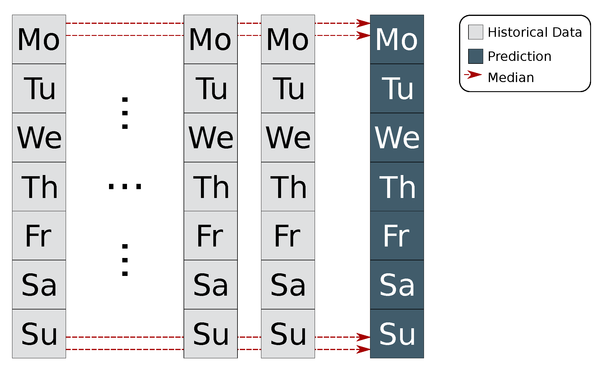
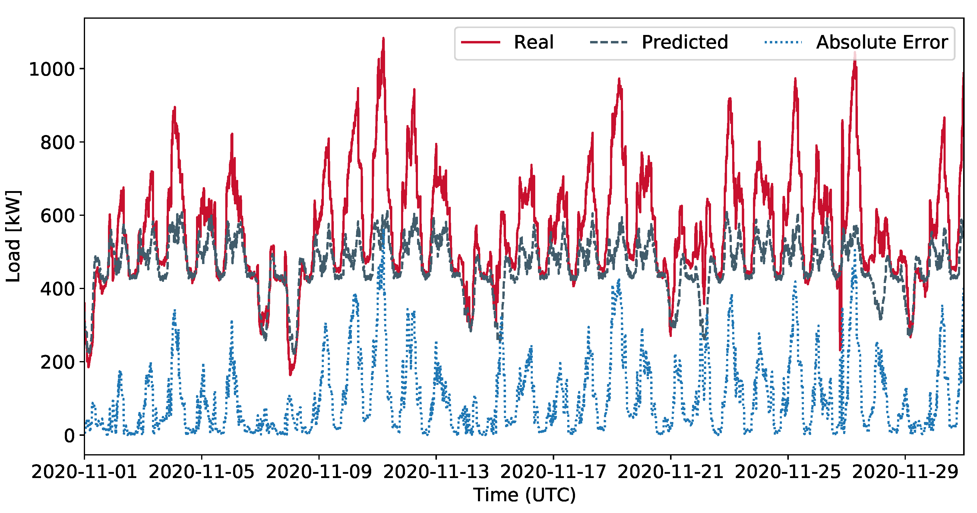
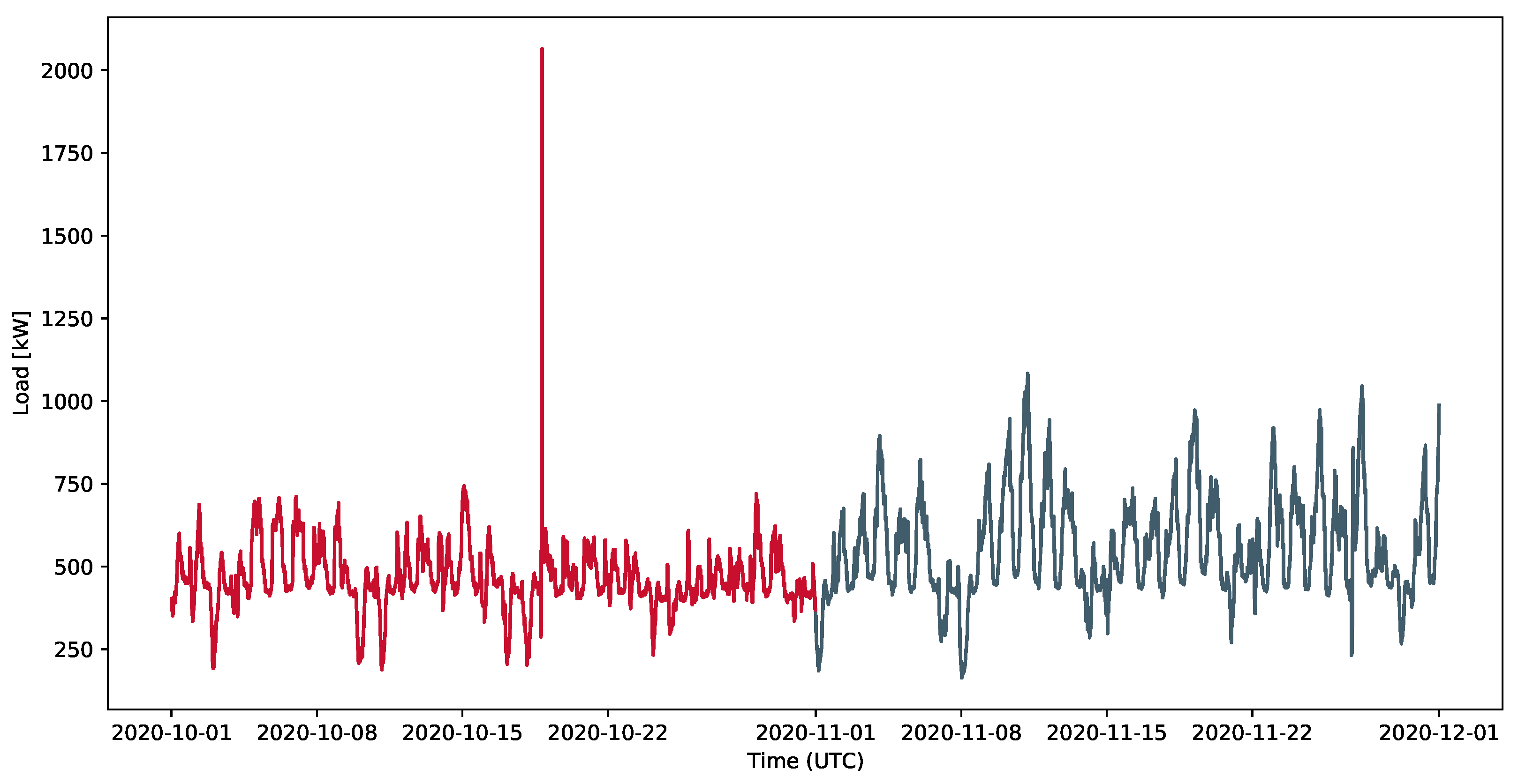
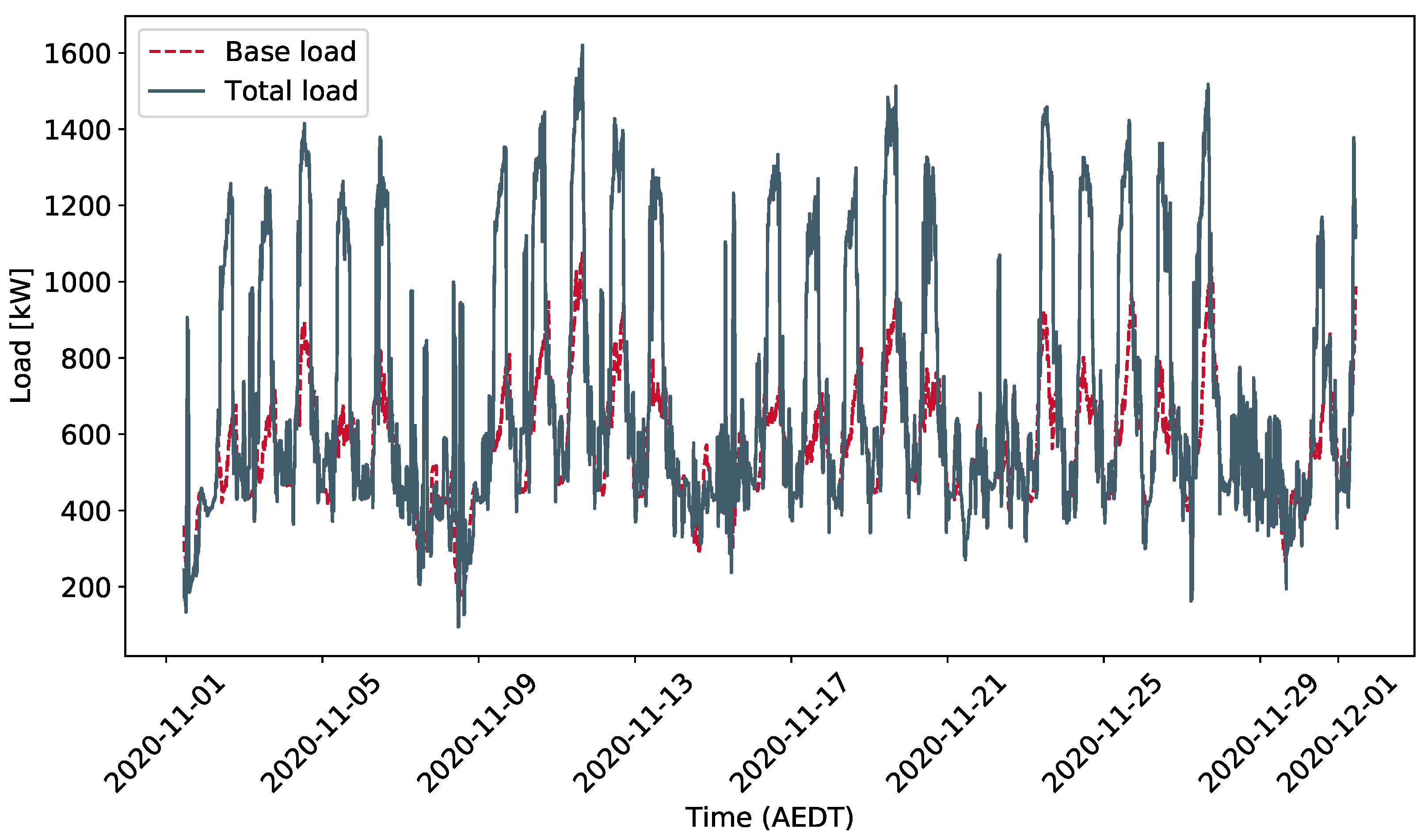
4.1. Building Load Prediction

For the building load prediction, a simple statistical approach, as illustrated in Figure 3, is used.

The load at a certain time step of a week is predicted as the median over the load values at the corresponding time steps of the historical data, taking into account the data from eight weeks prior to the month to be predicted. For example, the load on a Monday at 10:00 a.m. is predicted to be the median over the loads at 10:00 a.m. on Mondays in the historical data. We consider only eight weeks of historical data since the characteristics of the load data have been continuously changing since April 2020 due to restrictions in response to the COVID-19 pandemic. Time steps for which no load data are available are not included in the computation of the median value. If all eight historical load values are not available, a load of zero is predicted. Please note that this turned out to be disadvantageous for the data in the second phase of the challenge since in contrast to the data from the first phase, there are a lot of time steps without measurements in the previous eight weeks, resulting in a notable underestimation of the load. An improvement, which would have yielded better results on the phase-two data and similar results on the phase-one data, would be to use the median for all weeks of the historical data at the time steps for which no data in the previous eight weeks were available. However, in the present manuscript, we report the results of the original approach we used in the challenge.

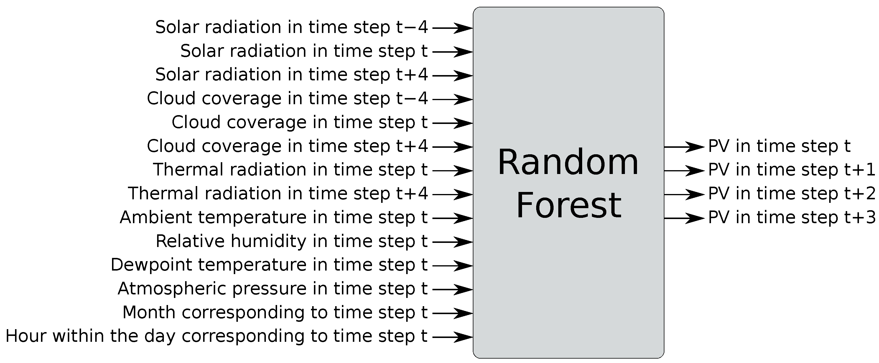
4.2. Photovoltaics Prediction

For the PV prediction, we use a machine learning approach with mainly weather data as input features. We cleaned the historical data for each of the six PV systems and removed days that contain (manually determined) outliers as well as days containing only zero-production entries. Furthermore, we shifted the weather data by −1 h since we noticed a certain offset between solar radiation and PV production. between solar radiation and PV production. In this way, the correlation between solar radiation and PV production in the training data is increased. For example, for the PV system Solar0, the Pearson correlation coefficient is 0.89 without the shift in the weather data and 0.92 with the shift. The preprocessed data were used to train a random forest with scikit-learn [5] default hyperparameter settings. Since only hourly weather data were available, and the prediction had to be made with a resolution of 15 min, the random forest predicts the PV production of a full hour in the form of four values (one per quarter of the hour). Let t denote a 15 min time step corresponding to the start of a full hour. The random forest predicts the PV production values at time steps $t,\cdots ,t+3$ based on 14 input features, as shown in Figure 4.

As one can see, not only weather data from the hour to be predicted is used as input, but also data from the previous and the following hour. We came up with the described approach by evaluating different approaches for the PV prediction for September 2020 and by choosing the approach that resulted in the smallest mean absolute errors. Besides random forest, we evaluated other models such as XGBoost, Gradient Boosting, k-nearest neighbors, and the automated machine learning approach TPOT [42], but all yielded inferior results. We evaluated different hyperparameter settings for the random forest, and we also evaluated different input features.

4.3. Optimization

We formulated the optimization problem as a mixed-integer linear programming problem and solved it with the help of the Gurobi solver [6]. A straightforward MILP formulation of the problem at hand would contain a large number of binary and integer variables, which typically has a negative impact on the solving time. Furthermore, the objective function contains a quadratic term (square of the peak power), which makes the problem even harder to solve. Thus, in order to accelerate the optimization and to be able to compute solutions of high quality in an acceptable time, we applied different measures:

(1)

Separate building assignment;

(2)

Variable reduction;

(3)

Solver parameter tuning;

(4)

Problem decomposition;

(5)

Linearization.

These are described in more detail in the following subsections.

4.3.1. Separate Building Assignment

The assignment of buildings to activities is separated from the actual optimization. In the optimization, it is only ensured that a feasible assignment exists (meaning there is a sufficient number of rooms allowing for the computation of a feasible building assignment for the activity schedule at hand) without computing a concrete assignment. This notably reduces the number of integer variables and constraints considered in the optimization. In a post-processing step, the assignment of buildings to activities is computed by solving a second MILP problem, which only has to find a feasible assignment (the objective function is fixed to zero). This second problem can be solved within a few seconds. Let $t_{min}$ and $t_{max}$ respectively be the first and last time steps of the working days of the first full week of the planning horizon ($t_{min}=96$ and $t_{max}=6\times 96-1$ in our use case). Furthermore, let $t^{open}$ and $t^{close}$ respectively denote the first and last time steps of the office hours during the day ($t^{open}=4\times 9$ and $t^{close}=4\times 17-1$ in our use case). Then, for a recurring activity $r\in R$, we can define the set $T_r$ of all possible start times in the first full week as follows:

$$T_r=\{t\in \{t_{min},\cdots ,t_{max}\}|t^{open}\le t\%96\le t\%96+D_r-1\le t^{close}\},$$

(5)

where % is the modulo operator. As each day has 96 time steps, $t\%96$ is the time step within a day. Analogously, for each once-off activity, we can define the set $T_o$ of all possible start times during the planning horizon as follows:

$$T_o=\{t\in \{0,\cdots ,T-1\}|t+D_o-1\le T-1\}.$$

(6)

Let $W_t\in \{0,\cdots ,6\}$ denote the weekday corresponding to time step t, where 0 stands for Monday, 1 stands for Tuesday, and so on. We use the following MILP formulation for the first problem (without the direct assignment of buildings to activities):

Problem P1:

$$min\sum _{t\in \{0,\cdots ,T-1\}}0.25·{\alpha }_t·L_t+\beta ·L^{max\_square}+\sum _{o\in O}\sum _{t\in T_o}{w}_{o,t}·F_{o,t}$$

(7)

with

$$w_{o,t}=\left\{\begin{array}{c}Re{m}^o,\mathrm{if}{W}_t<5\wedge t^{open}\le t\%96\le t\%96+D_o-1\le t^{close}\hfill \\ Re{m}^o-Pe{n}^o,\mathrm{else}\hfill \end{array}\right.,$$

(8)

subject to:

$$\begin{array}{ccc}\sum _{t\in T_r}{F}_{r,t}=1\hfill & & \hfill \hspace{1em}\hspace{1em}\hspace{1em}\hspace{1em}\hspace{1em}\hspace{1em}\hspace{1em}\hspace{1em}\hspace{1em}\hspace{1em}\hspace{1em}\hspace{1em}\hspace{1em}\hspace{1em}\hspace{1em}\hspace{1em}\hspace{1em}\hspace{1em}\hspace{1em}\forall r\in R,\end{array}$$

(9)

$$\begin{array}{ccc}\sum _{o\in T_o}{F}_{o,t}\le 1\hfill & & \hfill \hspace{1em}\hspace{1em}\hspace{1em}\hspace{1em}\hspace{1em}\hspace{1em}\hspace{1em}\hspace{1em}\hspace{1em}\hspace{1em}\hspace{1em}\hspace{1em}\hspace{1em}\hspace{1em}\hspace{1em}\hspace{1em}\hspace{1em}\hspace{1em}\hspace{1em}\forall o\in O,\end{array}$$

(10)

$$\begin{array}{ccc}\sum _{t\in T_r}{F}_{r,t}·W_t>\sum _{k\in T_k}{F}_{k,t}·W_t\hfill & & \hfill \hspace{1em}\hspace{1em}\hspace{1em}\hspace{1em}\hspace{1em}\hspace{1em}\hspace{1em}\hspace{1em}\hspace{1em}\hspace{1em}\hspace{1em}\hspace{1em}\hspace{1em}\hspace{1em}\forall r\in R,\forall k\in E_r,\end{array}$$

(11)

$$\begin{array}{ccc}\sum _{o\in T_o}{F}_{o,t}\le \sum _{k\in T_k}{F}_{k,t}\hfill & & \hfill \hspace{1em}\hspace{1em}\hspace{1em}\hspace{1em}\hspace{1em}\hspace{1em}\hspace{1em}\hspace{1em}\hspace{1em}\hspace{1em}\hspace{1em}\hspace{1em}\hspace{1em}\hspace{1em}\hspace{1em}\hspace{1em}\hspace{1em}\hspace{1em}\hspace{1em}\forall o\in O,\forall k\in E_o,\end{array}$$

(12)

$$\begin{array}{ccc}\sum _{o\in T_o}{F}_{o,t}·\lfloor t/96\rfloor >\sum _{k\in T_k}{F}_{k,t}·\lfloor t/96\rfloor -(T+1)·(1-\sum _{o\in T_o}{F}_{o,t})\hfill & & \hfill \hspace{1em}\hspace{1em}\hspace{1em}\hspace{1em}\hspace{1em}\hspace{1em}\forall o\in O,\forall k\in E_o,\end{array}$$

(13)

$$\begin{array}{cccc}\hfill & \sum _{r\in R}\sum _{k\in \{I_t-D_r+1,\cdots ,I_t\}\cap T_r}{F}_{r,k}·K_r^L+\hfill & & \hfill \\ & \sum _{o\in O}\sum _{k\in \{t-D_o+1,\cdots ,t\}\cap T_o}{F}_{o,k}·K_o^L\le \sum _{b\in B}{N}_b^L\hfill & & \hfill \hspace{1em}\hspace{1em}\hspace{1em}\hspace{1em}\hspace{1em}\hspace{1em}\hspace{1em}\hspace{1em}\hspace{1em}\hspace{1em}\hspace{1em}\forall t\in \{0,\cdots ,T-1\},\end{array}$$

(14)

$$\begin{array}{cccc}\hfill & \sum _{r\in R}\sum _{k\in \{I_t-D_r+1,\cdots ,I_t\}\cap T_r}{F}_{r,k}·K_r^S+\hfill & & \hfill \\ & \sum _{o\in O}\sum _{k\in \{t-D_o+1,\cdots ,t\}\cap T_o}{F}_{o,k}·K_o^S\le \sum _{b\in B}{N}_b^S\hfill & & \hfill \hspace{1em}\hspace{1em}\hspace{1em}\hspace{1em}\hspace{1em}\hspace{1em}\hspace{1em}\hspace{1em}\hspace{1em}\hspace{1em}\forall t\in \{0,\cdots ,T-1\},\end{array}$$

(15)

$$\begin{array}{ccc}c{h}_{s,t}+dc{h}_{s,t}\le 1\hfill & & \hfill \hspace{1em}\hspace{1em}\hspace{1em}\hspace{1em}\hspace{1em}\hspace{1em}\hspace{1em}\hspace{1em}\hspace{1em}\hspace{1em}\hspace{1em}\hspace{1em}\hspace{1em}\forall s\in S,\forall t\in \{0,\cdots ,T-1\},\end{array}$$

(16)

$$\begin{array}{ccc}{C}_{s,0}=C_s-0.25·dc{h}_{s,0}·M_s+0.25·c{h}_{s,0}·M_s\hfill & & \hfill \hspace{1em}\hspace{1em}\hspace{1em}\hspace{1em}\hspace{1em}\hspace{1em}\hspace{1em}\hspace{1em}\hspace{1em}\hspace{1em}\hspace{1em}\hspace{1em}\forall s\in S,\end{array}$$

(17)

$$\begin{array}{ccc}{C}_{s,t}=C_{s,t-1}-0.25·dc{h}_{s,t}·M_s+0.25·c{h}_{s,t}·M_s\hfill & & \hfill \hspace{1em}\hspace{1em}\hspace{1em}\hspace{1em}\hspace{1em}\forall s\in S,\forall t\in \{1,\cdots ,T-1\},\end{array}$$

(18)

$$\begin{array}{cccc}\hfill & L_t=L_t^{base}+\sum _{r\in R}\sum _{k\in \{I_t-D_r+1,\cdots ,I_t\}\cap T_r}{F}_{r,k}·L_r^A+\hfill & & \hfill \\ & \sum _{o\in O}\sum _{k\in \{t-D_o+1,\cdots ,t\}\cap T_o}{F}_{o,k}·L_o^A+\sum _{s\in S}(c{h}_{s,t}/{\gamma }_s-dc{h}_{s,t}·\sqrt{{\gamma }_s})·M_s\hfill & & \hfill \hspace{1em}\forall t\in \{0,\cdots ,T-1\},\end{array}$$

(19)

$$\begin{array}{ccc}{L}^{max}\ge L_t\hfill & & \hfill \hspace{1em}\hspace{1em}\hspace{1em}\hspace{1em}\hspace{1em}\hspace{1em}\hspace{1em}\hspace{1em}\hspace{1em}\hspace{1em}\hspace{1em}\hspace{1em}\forall t\in \{0,\cdots ,T-1\},\end{array}$$

(20)

$$\begin{array}{ccc}{L}^{max\_square}=L^{max}·L^{max},\hfill & & \hfill \hspace{1em}\hspace{1em}\hspace{1em}\hspace{1em}\hspace{1em}\hspace{1em}\hspace{1em}\hspace{1em}\hspace{1em}\hspace{1em}\hspace{1em}\end{array}$$

(21)

$$\begin{array}{ccc}{F}_{a,t}\in \{0,1\}\hfill & & \hfill \hspace{1em}\hspace{1em}\hspace{1em}\hspace{1em}\hspace{1em}\hspace{1em}\hspace{1em}\hspace{1em}\hspace{1em}\hspace{1em}\forall a\in A,\forall t\in T_a,\end{array}$$

(22)

$$\begin{array}{ccc}c{h}_{s,t},dc{h}_{s,t}\in \{0,1\}\hfill & & \hfill \hspace{1em}\hspace{1em}\hspace{1em}\hspace{1em}\hspace{1em}\hspace{1em}\hspace{1em}\forall s\in S,\forall t\in \{0,\cdots ,T-1\},\end{array}$$

(23)

$$\begin{array}{ccc}0\le C_{s,t}\le C_s\hfill & & \hfill \hspace{1em}\hspace{1em}\hspace{1em}\hspace{1em}\hspace{1em}\hspace{1em}\hspace{1em}\forall s\in S,\forall t\in \{0,\cdots ,T-1\}.\end{array}$$

(24)

The objective is to minimize the cost, as specified in Equation (4), where the $w_{o,t}$ in objective function (7) represents the remuneration received for starting the once-off activity o at time step t, as defined in Equation (8). The binary variables $F_{a,t}$ encode the start times of activities—if $F_{a,t}=1$, activity a starts at time step t. For each recurring activity $r\in R$, we only consider variables corresponding to possible start times in the first full week of the planning horizon (i.e., for t in $T_r$). Analogously, we only consider start times corresponding to time steps in $T_o$ for each once-off activity o. Constraints (9) and (10) ensure that exactly one start time for each recurring activity and at most one start time for each once-off activity are set. Constraint (11) ensures that recurring activities are started on a later weekday as compared to the corresponding preceding activities. Analogously, constraints (12) and (13) ensure for each once-off activity $o\in O$ that if o is scheduled, all preceding activities are also scheduled and take place at an earlier day than o. Please note that for $o\in O$, which is not scheduled, (12) and (13) are always satisfied. Constraint (14) ensures that there is no time step in which the running activities require more large rooms than what is available in the buildings in total. Similarly, constraint (15) ensures that there is a sufficient number of small rooms. The parameters $I_t$ used in (14) and (15) represent a mapping from a time step t to the corresponding time step in the first full week of the planning horizon:

$$I_t=\left\{\begin{array}{c}-1,\mathrm{if}t<t_{min}\vee t>t_{max\_rec}\hfill \\ t_{min}+(t-t_{min})\%(7·96),\mathrm{otherwise}\hfill \end{array}\right.,$$

(25)

where $t_{max\_rec}$ is the last time step of the last full week of the planning horizon ($t_{max\_rec}=29\times 96$ in our use case). Time steps that do not belong to a full week of the planning horizon are mapped to −1 to take into account that in these time steps, recurring activities cannot be active. The binary variables $c{h}_{s,t}$ and $dc{h}_{s,t}$ encode the charging and discharging state, respectively, of stationary battery $s\in S$ in time step t. Constraint (16) ensures that a battery does not charge and discharge at the same time. Constraint (17) sets the battery levels after the first time step, and constraint (18) sets the battery levels after all other time steps. Constraint (19) sets the total load composed of the base load, the load resulting from activities, and the load resulting from the charging/discharging stationary batteries. Constraints (20) and (21) set the peak load and the squared peak load, respectively, and constraints (22)–(24) set the lower and upper bounds of decision variables.

After scheduling the start times of activities by solving problem P1, the assignment of buildings to scheduled activities is computed by solving a second MILP problem. For each recurring activity $r\in R$, let $t_r^{start}\in T_r$ denote the time step within the first full week of the planning horizon, in which r starts according to the result of the first problem P1. Furthermore, let $O^{sched}\subseteq O$ be the set of all once-off activities scheduled in the result of P1, and let $t_o^{start}$ be the start time step of activity $o\in O^{sched}$. The assignment of buildings to activities is computed by solving the following problem:

Problem P2:

$$min0$$

(26)

subject to:

$$\begin{array}{ccc}\sum _{b\in B}{V}_{a,b}=K_a^S+K_a^L\hfill & & \hfill \hspace{1em}\hspace{1em}\hspace{1em}\hspace{1em}\hspace{1em}\hspace{1em}\hspace{1em}\hspace{1em}\hspace{1em}\hspace{1em}\hspace{1em}\hspace{1em}\hspace{1em}\hspace{1em}\hspace{1em}\hspace{1em}\forall a\in R\cup O^{sched},\end{array}$$

(27)

$$\begin{array}{cccc}\hfill & \sum _{r\in R|K_r^S>0\wedge t_r^{start}\le I_t<t_r^{start}+D_r}{V}_{r,b}+\hfill & & \hfill \\ & \sum _{o\in O^{sched}|K_o^S>0\wedge t_o^{start}\le t<t_o^{start}+D_o}{V}_{o,b}\le N_b^S\hfill & & \hfill \hspace{1em}\hspace{1em}\hspace{1em}\hspace{1em}\hspace{1em}\hspace{1em}\hspace{1em}\forall b\in B,\forall t\in \{0,\cdots ,T-1\},\end{array}$$

(28)

$$\begin{array}{cccc}\hfill & \sum _{r\in R|K_r^L>0\wedge t_r^{start}\le I_t<t_r^{start}+D_r}{V}_{r,b}+\hfill & & \hfill \\ & \sum _{o\in O^{sched}|K_o^L>0\wedge t_o^{start}\le t<t_o^{start}+D_o}{V}_{o,b}\le N_b^L\hfill & & \hfill \hspace{1em}\hspace{1em}\hspace{1em}\hspace{1em}\hspace{1em}\hspace{1em}\hspace{1em}\hspace{1em}\forall b\in B,\forall t\in \{0,\cdots ,T-1\},\end{array}$$

(29)

The objective function is constant zero since we are only interested in finding a feasible building assignment. The assignment of buildings is encoded in integer variables $V_{a,b}$, which denotes the number of rooms of building $b\in B$ that is assigned to activity $a\in A$. Constraint (27) ensures that to each recurring activity and each scheduled once-off activity, a sufficient number of rooms is assigned. Constraints (28) and (29) ensure that at each time step t, the respectively small and large rooms used in a building $b\in B$ are not more than what is available in b. Please remember that each activity $a\in A$ uses either only small rooms or only large rooms, and thus either $K_a^S$ or $K_a^L$ is zero.

4.3.2. Variable Reduction

In problem P1, only variables $F_{a,t}$ corresponding to possible start times t of activity a defined by the set $T_a$ (Equations (5) and (6)) are considered. However, taking into account the precedence constraints, the number of possible start times and thus the number of variables can be further reduced. For example, if a recurring activity has at least one preceding activity, then it cannot start on a Monday, and we can exclude from the problem all variables corresponding to start times of that activity which occur on a Monday. The first possible start day $d_a^{first}$ of the first full week (for recurring activities) or of the full planning horizon (for once-off activities) can be computed recursively for an activity a, as outlined in Algorithm 1.

Analogously, the last possible start day $d_a^{last}$ of the first full week or of the full planning horizon can be computed. We reduce the number of variables in problem P1 by considering, for each recurring activity $r\in R$, only start times in the set $T_r^{\prime }$:

$$T_r^{\prime }=\{t\in \{t_{min},\cdots ,t_{max}\}|t^{open}\le t\%96\le t\%96+D_r-1\le t^{close}\wedge d_r^{first}\le W.t\le d_r^{last}\},$$

(30)

and for each once-off activity $o\in O$, only start times in the set $T_o^{\prime }$:

$$T_o^{\prime }=\{t\in \{0,\cdots ,T-1\}|t+D_o-1\le T-1\wedge d_o^{first}\le \lfloor t/96\rfloor \le d_o^{last}\}.$$

(31)

Algorithm 1: Computation of first possible start day.

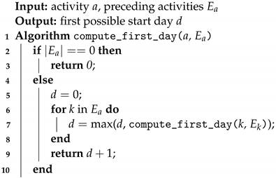
4.3.3. Solver Parameter Tuning

MILP solvers such as the Gurobi solver have a large number of parameters, whose settings can have a notable impact on the performance. The default parameter settings typically yield a good average performance through arbitrary problem instances. However, when restricted to a certain class or domain of problems, other settings might be superior [43]. Gurobi has a built-in parameter tuning tool. We used this tool to determine appropriate parameter settings for some problem instances of phase one of the challenge, and we employed the resulting settings in all further optimizations. In the parameter settings, the parameter PreSparsify is set to 0 and the parameter VarBranch is set to 1, while all other parameters are left at their default values.

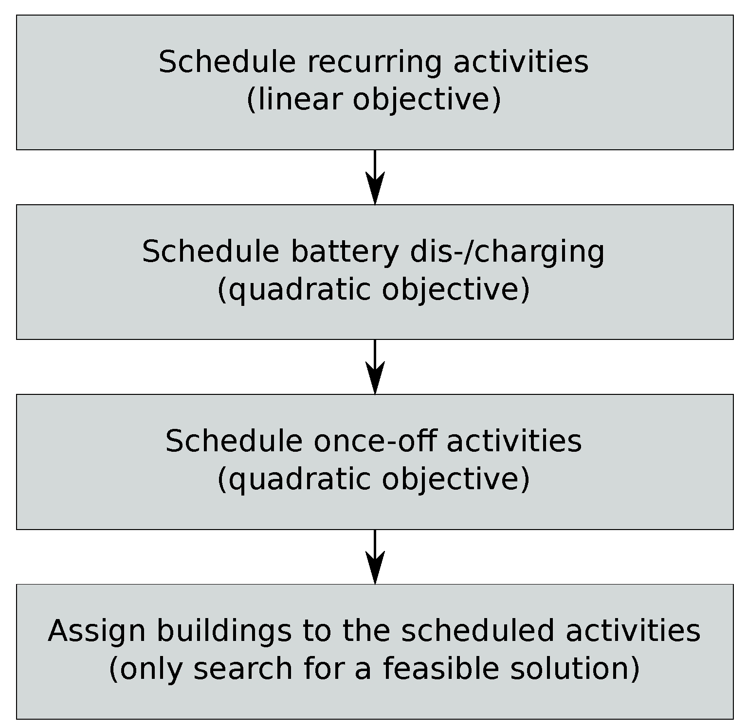
4.3.4. Problem Decomposition

Even after separating the building assignment from the actual optimization and reducing the number of variables, considering all activities and stationary batteries simultaneously in the optimization results in a large number of binary variables. Hence, we further accelerate the optimization by splitting the problem into multiple smaller and easier to solve sub-problems: First, the schedule of recurring activities is optimized, assuming that the batteries are not used and that no once-off activities take place. This means that problem P1 is solved, assuming that no once-off activities and no stationary batteries exist. After this first sub-problem is solved, the battery charging is optimized by fixing the start times of recurring activities according to the result of the first sub-problem and assuming that no once-off activities take place. Then, the schedule of the once-off activities is optimized by fixing the schedules of stationary batteries and recurring activities according the results of the second sub-problem. By decomposing the problem into easier sub-problems, a notable acceleration can be achieved. Furthermore, it can be considered that the described problem decomposition only has a minor impact on the solution quality. Recurring activities can be scheduled only within office hours, and it hardly makes sense to schedule additional once-off activities within office hours since this would increase the peak load. Thus, the fact that recurring activities and once-off activities are treated separately should have no significant impact on the solution. In the experiments, the order of the last two sub-problem—first batteries and then once-off activities—yielded better results than the inverse order.

4.3.5. Linearization

In the optimization of the schedule of recurring activities, we do not use the original quadratic objective function. Instead, the peak load is linearly included in the objective function, with a high coefficient of 1000. This means that in the first sub-problem, constraint (21) is not included and objective function (7) is replaced by the following objective function:

$$min\sum _{t\in \{0,\cdots ,T-1\}}0.25·{\alpha }_t·L_t+1000·L^{max}+\sum _{o\in O}\sum _{t\in T_o}{w}_{o,t}·F_{o,t}.$$

(32)

The scheduling of the recurring activities is the hardest of the three sub-problems (at least for the considered problem instances), and by linearizing its objective function, it can be accelerated with only a minor impact on the solution quality.

The complete optimization consists of the execution of the steps illustrated in Figure 5.

5. Simulation Experiments

5.1. Predictions

We computed forecasts of the individual loads and productions in November 2020, as described in Section 4.1 and Section 4.2, and derived a prediction of the total base load according Equation (1).

Table 2. Mean absolute error (MAE) and root mean squared error (RMSE) of predictions of individual loads/productions and total load, as determined by our approach and the winning submission of the challenge.

Load/Production	Our Approach		Winning Submission
	MAE	RMSE	MAE	RMSE
Building0	37.31	52.68	34.46	48.11
Building1	2.14	3.22	1.89	3.15
Building3	68.27	103.78	61.38	95.19
Building4	0.69	0.92	0.56	0.76
Building5	6.25	12.58	8.92	10.53
Building6	2.47	4.45	2.40	4.44
Solar0	3.31	6.06	3.19	5.46
Solar1	0.61	1.20	0.65	1.22
Solar2	0.64	1.23	0.70	1.26
Solar3	0.78	1.40	0.75	1.29
Solar4	0.37	0.72	0.43	0.77
Solar5	1.97	3.77	2.16	3.85
Total Load	102.17	144.83	82.49	120.72

shows the resulting mean absolute errors (MAE) and root mean squared errors (RMSE) for the different sub-loads and the total load. For comparison, the prediction errors of the submission that won the competition are also shown in Table 2. The winning team (Rasul Esmaeilbeigi and Mahdi Abolghasemi) made their final submission publicly available (the winning submission is available under https://github.com/resmaeilbeigi/IEEE_CIS_3rd_Technical_Challenge_Optimiser (accessed on 15 May 2022)). They used an ensemble machine learning approach for the prediction of load and PV production.

As one can see, the PV prediction is very accurate since the PV production is strongly correlated with the weather, which is used as input for the prediction, and the errors resulting from our approach are in the same range as the errors of the winning submission. The building load prediction is more challenging—especially due to the impact of the COVID-19 measures—and the winning submission notably outperforms our approach on the building load. Figure 6 shows the real and predicted total load together with the corresponding absolute prediction errors.

As one can see, there is a notable tendency to underestimate the load. One reason for this, as already described in Section 4.1, is that predicting a load of zero, if no corresponding data in the eight historical weeks is available, results in an underestimation of the load (the improvement described in Section 4.1 would reduce the MAE for the total load to 95.83). Furthermore, there is an unexpected increase in the load in November, as can be seen in Figure 7, which is hard to predict. That is why in the winning submission, the total load is underestimated as well. The outlier in the October load shown in Figure 7 is obviously the result of an erroneous measurement.

5.2. Optimizations

In order to investigate the effect of different improvements in optimization described in Section 4.3, we executed optimizations on six problem instances in phase two of the challenge. The prediction shown in Figure 6 is used as input for the optimizations. We ran the optimizations with six different settings:

• c_q_f: Combined optimization of all activities and batteries with quadratic objective and a full number of binary variables;
• c_q_r: Combined optimization of all activities and batteries with quadratic objective and a reduced number of binary variables (improvement (2));
• c_l_r: Combined optimization of all activities and batteries with linear objective (improvement (5)) and a reduced number of binary variables (improvement (2));
• s_q_f: Separate optimizations of recurring activities, batteries, and once-off activities (improvement (4)) with quadratic objective and the full number of binary variables;
• s_q_r: Separate optimizations of recurring activities, batteries, and once-off activities (improvement (4)) with quadratic objective and a reduced number of binary variables (improvement (2));
• s_l_r: Separate optimizations of recurring activities, batteries, and once-off activities (improvement (4)) with linear objective for recurring activities (improvement (5)) and a reduced number of binary variables (improvement (2)).

Improvements (1) and (3) (separate building assignment and parameter tuning) are applied in all settings. With the setting c_l_r, the objective function of the complete optimization, and not only of the scheduling of recurring activities, is linearized since the problem is not decomposed. We ran the experiments on a 2.1 GHz Intel Xeon Silver 4110 CPU with 8 cores and 93 GB RAM and used version 9.1.0 of Gurobi as solver. For the combined optimizations, a time limit of 15 min was set, and for the separate optimizations, time limits of 12 min, 1.5 min, and 1.5 min were respectively set for the optimizations of recurring activities, once-off activities, and batteries.

Table 3. Optimization results with different settings on six problem instances, with a time limit of 15 min for the total optimization.

Problem	c_q_f	c_q_r	c_l_r	s_q_f	s_q_r	s_l_r
small0	26,299	25,971	25,006	24,489	24,669	24,399
small1	26,092	24,920	24,211	23,414	23,414	23,443
small2	25,696	26,145	23,706	23,485	23,665	23,341
large0	25,184	25,105	23,575	23,859	23,839	23,640
large1	25,364	25,365	24,096	24,314	24,283	23,925
large2	24,209	24,168	23,028	23,021	22,972	22,651
Mean	25,474	25,279	23,937	23,764	23,807	23,567

shows the resulting electricity costs on the predicted load.

As one can see, the setting s_l_r (which corresponds to our final setting), yielded the best mean objective. The linearization of the objective function (c_l_r vs. c_q_r and s_l_r vs. s_q_r) and the separate optimizations (s_* vs. c_*) yielded notable improvements. However, the benefit of the variable reduction (c_q_r vs. c_q_f and s_q_r vs. s_q_f) was small, and for the separate optimization, it even had a negative impact on the mean objective. The reason for this is that the solver is able to automatically reduce the number of variables during the pre-solving phase. This can be seen in

Table 4. Number of variables of different types in the first sub-problem, with the settings s_q_f and s_q_r before and after pre-solving for two problem instances.

Problem	s_q_f			s_q_r
	Continuous	Integer	Binary	Continuous	Integer	Binary
Before Pre-solving
small0	2882	6770	6770	2882	2922	2922
large0	2882	27,320	27,320	2882	13,222	13,222
After Pre-solving
small0	135	2935	2922	143	2935	2922
large0	137	13,235	13,222	137	13,235	13,222

, which shows the number of variables in the first sub-problem with the settings s_q_f and s_q_r before and after the pre-solving for two problem instances.

Before the pre-solving, the number of binary variables is significantly lower with setting s_q_r as compared to setting s_q_f. However, after pre-solving, the number of binary variables is the same for both settings.

In a further experiment, we observed the impact of the prediction error on the optimization results.

Table 5. Cost of the predicted and real load in AUD, resulting from optimizations on predicted and real load for problem instance small0.

	Pred-Pred	Pred-Real	Real-Real
Peak cost	6588	14,549	10,842
Energy cost	17,870	21,262	21,237
Once-off profit	59	59	619
Total cost	24,399	35,752	31,460

shows the cost of the predicted and real load for problem instance small0, when the optimization is performed on the prediction (pred-pred and pred-real, respectively), and the cost of the real load, when the optimization is performed on the real load (real-real). The optimizations were completed using the setting s_l_r and the previously stated time limits.

Not surprisingly, the cost of the predicted load notably underestimates the real cost since, as discussed in Section 5.1, the prediction notably underestimates the load. While the real energy costs are basically identical for the optimizations on the predicted and the real load, the optimization on the real load yields a notably lower peak cost, resulting in a total cost that is about 12% lower as compared to the optimization on the predicted load. Thus, one can conclude that the error in the prediction has a remarkable negative impact on the optimization results.

We executed optimizations on all ten problem instances with higher time limits, using settings analogous to those used to compute our final submission to the challenge. Again, the optimizations were performed on a 2.1 GHz Intel Xeon Silver 4110 CPU with 8 cores and 93 GB RAM, with version 9.1.0 of Gurobi. The time limits for the optimizations of recurring activities, batteries, and once-off activities were set to 150 min, 15 min, and 15 min, respectively.

Table 6. Percentage optimality gaps of sub-optimization on all ten problem instances.

Problem	Recurring	Batteries	Once-Off
small0	2.5%	0.8%	2.2%
small1	0.0%	0.6%	2.1%
small2	0.0%	0.5%	2.0%
small3	0.0%	0.7%	0.0%
small4	0.0%	0.7%	0.0%
large0	1.4%	0.7%	4.9%
large1	1.5%	1.0%	4.7%
large2	1.6%	0.5%	4.2%
large3	1.6%	0.9%	4.4%
large4	1.6%	1.1%	3.7%

shows the resulting optimality gaps for the three sub-problems of the different problem instances, as reported by the solver.

It can be seen that for four of the small problem instances, the sub-problem of scheduling the recurring activities could be solved exactly. Not surprisingly, the optimizations of large instances yielded higher gaps than the optimizations of small instances. The optimization of once-off activities is the sub-problem yielding the highest gaps. However, as one can see, the optimality gaps are generally small, and one has to keep in mind that these are only worst-case gaps and that the actual gaps might be smaller.

Details of the results for the ten problem instances can be found in

Table 7. Detailed results of our approach on all ten problem instances.

Problem	OS	PC (AUD)	EC (AUD)	OP (AUD)	TC (AUD)
small0	7	13,195	21,283	29	34,449
small1	19	13,130	20,865	251	33,744
small2	2	13,081	20,833	60	33,855
small3	20	12,533	20,994	267	33,259
small4	20	13,825	20,924	869	33,880
large0	6	13,025	21,225	78	34,173
large1	7	13,374	21,290	43	34,622
large2	11	12,075	20,919	29	32,964
large3	8	12,467	21,029	42	33,454
large4	30	13,074	21,233	236	34,071

. It shows the number of scheduled once-off activities (OS), the peak cost (PC), the energy cost (EC), the once-off profit (OP), and the total cost (TC) of the real load for all problem instances. The sum of the total cost for all instances is AUD 338,470. Please note that this is a little bit smaller than the total cost resulting from our last submission to the challenge (AUD 339,160) since we repeated the optimizations for the present manuscript. For comparison,

Table 8. Detailed results of the winning approach on all ten problem instances and percentage gaps of total costs as compared to our approach.

Problem	OS	PC (AUD)	EC (AUD)	OP (AUD)	TC (AUD)	Gap (%)
small0	20	14,425	21,575	1491	34,509	+0.17
small1	19	13,726	21,131	1593	33,265	−1.42
small2	20	12,696	21,232	1500	32,428	−4.22
small3	20	13,289	21,181	1333	33,136	−0.37
small4	20	12,490	21,057	1056	32,490	−4.10
large0	99	12,912	21,619	1889	32,643	−4.48
large1	100	13,244	21,658	1847	33,055	−4.53
large2	97	12,160	21,238	1686	31,712	−3.80
large3	100	12,502	21,443	1725	32,219	−3.69
large4	94	12,927	21,602	1626	32,903	−3.43

shows the detailed results of the submission that won the competition, and for each problem instance, the percentage gap of the total cost as compared to the result of our approach in Table 7. The winning team used for the optimization a stochastic MILP approach based on predictions with errors shown in Table 2. The winning submission yields lower total cost (TC) than our approach on all problem instances, except for the first instance, although the peak cost (PC) and energy cost (EC) are higher on many instances. As one can see, the profit from once-off activities (OP) is also notably higher than in our results. Thus, it seems like the main advantage of the winning approach compared to our approach is that it is better in handling the once-off activities.

Figure 8 shows the predicted base load and total load resulting from our schedule for problem instance small1.

Once-off activities are scheduled on weekends and at the end of the planning horizon (on a Monday and part of a Tuesday) since no recurring activities take place at these times, and thus the peak load is not increased by the once-off activities. The load of the recurring activities on the working days of the full weeks of the planning horizon is well-distributed, resulting in similar peak loads on all days of the full weeks. Figure 9 shows the real base load and the total load resulting from the same schedule. As one can see, the peaks are no longer similar on the different working days of the full weeks, and the total peak occurs on the 11th of November (which is also the case for all other problem instances).

6. Summary and Conclusions

In the present paper, we provided a detailed description and evaluation of our approach to the prediction and optimization problem formulated in the 2021 “IEEE-CIS Technical Challenge on Predict + Optimize for Renewable Energy Scheduling”. In order to deal with the influence of the COVID-19 measures on the load data and the resulting limited amount of useful training data, we opted for a simple but robust statistical approach for the load forecasting. The forecast of photovoltaic production was executed with the help of a machine learning model based on weather data. The complex optimization problem was tackled by formulating it as a mixed-integer linear programming problem and solving it with the help of the Gurobi solver. Different measures to accelerate the optimization were taken, and their benefits were demonstrated in experiments. An analysis of the forecasts revealed that while the forecast of the photovoltaic production is very accurate, the load forecast notably underestimates the load. In addition to an unpredictable increase in the load, an internal issue of the used approach, which would be easy to correct, was identified as a reason for this. The experiments showed that the prediction errors have a notable impact on the optimization results. Nevertheless, the used approach proved to be competitive and yielded the third rank in the final leaderboard of the challenge. Hence, it is fair to assume that the other teams had similar issues with the load forecast.

References

1. Tol, R.S. Europe’s Climate Target for 2050: An Assessment. Intereconomics 2021, 56, 330–335. [Google Scholar] [CrossRef] [PubMed]
2. Roesch, M.; Linder, C.; Zimmermann, R.; Rudolf, A.; Hohmann, A.; Reinhart, G. Smart Grid for Industry Using Multi-Agent Reinforcement Learning. Appl. Sci. 2020, 10, 6900. [Google Scholar] [CrossRef]
3. Stadie, M.; Rodemann, T.; Burger, A.; Jomrich, F.; Limmer, S.; Rebhan, S.; Saeki, H. V2B Vehicle to Building Charging Manager. In Proceedings of the EVTeC: 5th International Electric Vehicle Technology Conference 2021, Yokohama, Japan, 24–26 May 2021. [Google Scholar]
4. Bergmeir, C. IEEE-CIS Technical Challenge on Predict+Optimize for Renewable Energy Scheduling. 2021. Available online: https://ieee-dataport.org/competitions/ieee-cis-technical-challenge-predictoptimize-renewable-energy-scheduling (accessed on 16 May 2022).
5. Pedregosa, F.; Varoquaux, G.; Gramfort, A.; Michel, V.; Thirion, B.; Grisel, O.; Blondel, M.; Prettenhofer, P.; Weiss, R.; Dubourg, V.; et al. Scikit-learn: Machine Learning in Python. J. Mach. Learn. Res. 2011, 12, 2825–2830. [Google Scholar]
6. Gurobi Optimization, LLC. Gurobi Optimizer Reference Manual; Gurobi Optimization, LLC: Houston, TX, USA, 2022. [Google Scholar]
7. Mamun, A.A.; Sohel, M.; Mohammad, N.; Haque Sunny, M.S.; Dipta, D.R.; Hossain, E. A Comprehensive Review of the Load Forecasting Techniques Using Single and Hybrid Predictive Models. IEEE Access 2020, 8, 134911–134939. [Google Scholar] [CrossRef]
8. Nti, I.K.; Teimeh, M.; Nyarko-Boateng, O.; Adekoya, A.F. Electricity load forecasting: A systematic review. J. Electr. Syst. Inf. Technol. 2020, 7, 1–19. [Google Scholar] [CrossRef]
9. Groß, A.; Lenders, A.; Schwenker, F.; Braun, D.A.; Fischer, D. Comparison of short-term electrical load forecasting methods for different building types. Energy Inform. 2021, 4, 1–16. [Google Scholar]
10. Antonanzas, J.; Osorio, N.; Escobar, R.; Urraca, R.; de Pison, F.M.; Antonanzas-Torres, F. Review of photovoltaic power forecasting. Sol. Energy 2016, 136, 78–111. [Google Scholar] [CrossRef]
11. Ahmed, R.; Sreeram, V.; Mishra, Y.; Arif, M. A review and evaluation of the state-of-the-art in PV solar power forecasting: Techniques and optimization. Renew. Sustain. Energy Rev. 2020, 124, 1–26. [Google Scholar] [CrossRef]
12. Schmitt, T.; Rodemann, T.; Adamy, J. Multi-objective model predictive control for microgrids. Automatisierungstechnik 2020, 68, 687–702. [Google Scholar] [CrossRef]
13. Altin, N.; Eyimaya, S.E. A Review of Microgrid Control Strategies. In Proceedings of the 2021 10th International Conference on Renewable Energy Research and Application, Istanbul, Turkey, 26–29 September 2021; pp. 412–417. [Google Scholar] [CrossRef]
14. Wang, Q.; Liu, X.; Du, J.; Kong, F. Smart Charging for Electric Vehicles: A Survey From the Algorithmic Perspective. IEEE Commun. Surv. Tutor. 2016, 18, 1500–1517. [Google Scholar] [CrossRef] [Green Version]
15. Naharudinsyah, I.; Limmer, S. Optimal Charging of Electric Vehicles with Trading on the Intraday Electricity Market. Energies 2018, 11, 1416. [Google Scholar] [CrossRef] [Green Version]
16. Espín-Sarzosa, D.; Palma-Behnke, R.; Núñez Mata, O. Energy Management Systems for Microgrids: Main Existing Trends in Centralized Control Architectures. Energies 2020, 13, 547. [Google Scholar] [CrossRef] [Green Version]
17. Hoke, A.; Brissette, A.; Chandler, S.; Pratt, A.; Maksimović, D. Look-ahead economic dispatch of microgrids with energy storage, using linear programming. In Proceedings of the 2013 1st IEEE Conference on Technologies for Sustainability (SusTech), Portland, OR, USA, 1–2 August 2013; pp. 154–161. [Google Scholar] [CrossRef]
18. Torres, D.; Crichigno, J.; Padilla, G.; Rivera, R. Scheduling coupled photovoltaic, battery and conventional energy sources to maximize profit using linear programming. Renew. Energy 2014, 72, 284–290. [Google Scholar] [CrossRef] [Green Version]
19. Jiang, Q.; Xue, M.; Geng, G. Energy Management of Microgrid in Grid-Connected and Stand-Alone Modes. IEEE Trans. Power Syst. 2013, 28, 3380–3389. [Google Scholar] [CrossRef]
20. Khani, H.; Zadeh, M.R.D. Online Adaptive Real-Time Optimal Dispatch of Privately Owned Energy Storage Systems Using Public-Domain Electricity Market Prices. IEEE Trans. Power Syst. 2015, 30, 930–938. [Google Scholar] [CrossRef]
21. Sani Hassan, A.; Cipcigan, L.; Jenkins, N. Optimal battery storage operation for PV systems with tariff incentives. Appl. Energy 2017, 203, 422–441. [Google Scholar] [CrossRef]
22. Koller, M.; Borsche, T.; Ulbig, A.; Andersson, G. Defining a degradation cost function for optimal control of a battery energy storage system. In Proceedings of the 2013 IEEE Grenoble Conference, Grenoble, France, 16–20 June 2013; pp. 1–6. [Google Scholar] [CrossRef]
23. Zhou, B.; Liu, X.; Cao, Y.; Li, C.; Chung, C.Y.; Chan, K.W. Optimal scheduling of virtual power plant with battery degradation cost. IET Gener. Transm. Distrib. 2016, 10, 712–725. [Google Scholar] [CrossRef]
24. Xu, B.; Zhao, J.; Zheng, T.; Litvinov, E.; Kirschen, D.S. Factoring the Cycle Aging Cost of Batteries Participating in Electricity Markets. IEEE Trans. Power Syst. 2018, 33, 2248–2259. [Google Scholar] [CrossRef] [Green Version]
25. Maheshwari, A.; Paterakis, N.G.; Santarelli, M.; Gibescu, M. Optimizing the operation of energy storage using a non-linear lithium-ion battery degradation model. Appl. Energy 2020, 261, 114360. [Google Scholar] [CrossRef]
26. Abdulla, K.; de Hoog, J.; Muenzel, V.; Suits, F.; Steer, K.; Wirth, A.; Halgamuge, S. Optimal Operation of Energy Storage Systems Considering Forecasts and Battery Degradation. IEEE Trans. Smart Grid 2018, 9, 2086–2096. [Google Scholar] [CrossRef]
27. Li, Y.; Vilathgamuwa, D.M.; Choi, S.S.; Farrell, T.W.; Tran, N.T.; Teague, J. Nonlinear Model Predictive Control of Photovoltaic-Battery System for Short-Term Power Dispatch. In Proceedings of the IECON 2018—44th Annual Conference of the IEEE Industrial Electronics Society, Washington, DC, USA, 21–23 October 2018; pp. 1884–1889. [Google Scholar] [CrossRef] [Green Version]
28. Aaslid, P.; Belsnes, M.M.; Fosso, O.B. Optimal microgrid operation considering battery degradation using stochastic dual dynamic programming. In Proceedings of the 2019 International Conference on Smart Energy Systems and Technologies (SEST), Porto, Portugal, 9–11 September 2019; pp. 1–6. [Google Scholar] [CrossRef] [Green Version]
29. Kumar, R.; Wenzel, M.J.; Ellis, M.J.; ElBsat, M.N.; Drees, K.H.; Zavala, V.M. A Stochastic Model Predictive Control Framework for Stationary Battery Systems. IEEE Trans. Power Syst. 2018, 33, 4397–4406. [Google Scholar] [CrossRef]
30. Cai, J.; Zhang, H.; Jin, X. Aging-aware predictive control of PV-battery assets in buildings. Appl. Energy 2019, 236, 478–488. [Google Scholar] [CrossRef]
31. Logenthiran, T.; Srinivasan, D.; Shun, T.Z. Demand Side Management in Smart Grid Using Heuristic Optimization. IEEE Trans. Smart Grid 2012, 3, 1244–1252. [Google Scholar] [CrossRef]
32. Ahmad, A.; Khan, A.; Javaid, N.; Hussain, H.M.; Abdul, W.; Almogren, A.; Alamri, A.; Azim Niaz, I. An Optimized Home Energy Management System with Integrated Renewable Energy and Storage Resources. Energies 2017, 10, 549. [Google Scholar] [CrossRef] [Green Version]
33. Hussain, H.M.; Javaid, N.; Iqbal, S.; Hasan, Q.U.; Aurangzeb, K.; Alhussein, M. An Efficient Demand Side Management System with a New Optimized Home Energy Management Controller in Smart Grid. Energies 2018, 11, 190. [Google Scholar] [CrossRef] [Green Version]
34. Lezama, F.; Soares, J.; Canizes, B.; Vale, Z. Flexibility management model of home appliances to support DSO requests in smart grids. Sustain. Cities Soc. 2020, 55, 102048. [Google Scholar] [CrossRef]
35. Rana, M.J.; Rahi, K.H.; Ray, T.; Sarker, R. An efficient optimization approach for flexibility provisioning in community microgrids with an incentive-based demand response scheme. Sustain. Cities Soc. 2021, 74, 103218. [Google Scholar] [CrossRef]
36. Sou, K.C.; Weimer, J.; Sandberg, H.; Johansson, K.H. Scheduling smart home appliances using mixed integer linear programming. In Proceedings of the 2011 50th IEEE Conference on Decision and Control and European Control Conference, Orlando, FL, USA, 12–15 December 2011; pp. 5144–5149. [Google Scholar] [CrossRef] [Green Version]
37. Bradac, Z.; Kaczmarczyk, V.; Fiedler, P. Optimal Scheduling of Domestic Appliances via MILP. Energies 2015, 8, 217–232. [Google Scholar] [CrossRef]
38. Taik, S.; Kiss, B. Smart Household Electricity Usage Optimization Using MPC and MILP. In Proceedings of the 2019 22nd International Conference on Process Control (PC19), Strbske Pleso, Slovakia, 11–14 June 2019; pp. 31–36. [Google Scholar] [CrossRef]
39. Limmer, S.; Lezama, F.; Soares, J.A.; Vale, Z. Coordination of Home Appliances for Demand Response: An Improved Optimization Model and Approach. IEEE Access 2021, 9, 146183–146194. [Google Scholar] [CrossRef]
40. Enrich, R.; Skovron, P.; Tolos, M.; Torrent-Moreno, M. Microgrid management based on economic and technical criteria. In Proceedings of the 2012 IEEE International Energy Conference and Exhibition (ENERGYCON), Florence, Italy, 9–12 September 2012; pp. 551–556. [Google Scholar] [CrossRef]
41. Alghamdi, H.; Alsubait, T.; Alhakami, H.; Baz, A. A review of optimization algorithms for university timetable scheduling. Eng. Technol. Appl. Sci. Res. 2020, 10, 6410–6417. [Google Scholar] [CrossRef]
42. Olson, R.S.; Bartley, N.; Urbanowicz, R.J.; Moore, J.H. Evaluation of a Tree-based Pipeline Optimization Tool for Automating Data Science. In Proceedings of the Genetic and Evolutionary Computation Conference (GECCO ’16), Denver, CO, USA, 20–24 July 2016; ACM: New York, NY, USA, 2016; pp. 485–492. [Google Scholar] [CrossRef] [Green Version]
43. Ishihara, T.; Limmer, S. Optimizing the Hyperparameters of a Mixed Integer Linear Programming Solver to Speed up Electric Vehicle Charging Control. In Applications of Evolutionary Computation, Proceedings of 23rd European Conference, EvoApplications 2020, Held as Part of EvoStar 2020, Seville, Spain, 15–17 April 2020; Lecture Notes in Computer Science; Springer: Cham, Switzerland, 2020; Volume 12104, pp. 37–53. [Google Scholar] [CrossRef]
Figure 1. Historical load and production data.
Energies 15 03718 g001
Figure 2. Half-hourly energy prices during the planning horizon.
Energies 15 03718 g002
Figure 3. Illustration of the load prediction approach.
Energies 15 03718 g003
Figure 4. Illustration of the PV prediction approach.
Energies 15 03718 g004
Figure 5. Workflow of the optimization.
Energies 15 03718 g005
Figure 6. Real and predicted November load and the corresponding absolute error.
Energies 15 03718 g006
Figure 7. Base load in October 2020 (red) and November 2020 (grey).
Energies 15 03718 g007
Figure 8. Predicted base load and total load resulting from the schedule for problem instance small1.
Energies 15 03718 g008
Figure 9. Real base load and total load resulting from the schedule for problem instance small1.
Energies 15 03718 g009