Short-Term Load Forecasting Based on the CEEMDAN-Sample Entropy-BPNN-Transformer

Abstract

Aiming at the problem that power load data are stochastic and that it is difficult to obtain accurate forecasting results by a single algorithm, in this paper, a combined forecasting method for short-term power load was proposed based on the Complete Ensemble Empirical Mode Decomposition with Adaptive Noise (CEEMDAN)-sample entropy (SE), the BP neural network (BPNN), and the Transformer model. Firstly, the power load data were decomposed into several power load subsequences with obvious complexity differences by using the CEEMDAN-SE. Then, BPNN and Transformer model were used to forecast the subsequences with low complexity and the subsequences with high complexity, respectively. Finally, the forecasting results of each subsequence were superimposed to obtain the final forecasting result. The simulation was taken from our proposed model and six forecasting models by using the load dataset from a certain area of Spain. The results showed that the MAPE of our proposed CEEMDAN-SE-BPNN-Transformer model was 1.1317%, while the RMSE was 304.40, which was better than the selected six forecasting models.

1. Introduction

The stable operation and economic dispatch in the power system relies heavily on the accurate forecasting of future loads [1]. The types of load forecasting can be divided into three categories, namely Short-term forecasting, Mid-term forecasting and Long-term forecasting [2]. Short-term power load forecasting is mainly used to arrange power generation plans and help relevant departments to establish reasonable power dispatching plans. Loads are strongly stochastic, and there are numerous factors affecting their load characteristics [3]. With the development of society and social economy, the scale of the power grid is becoming larger and larger, the number of devices keeps increasing, and the collection frequency of a smart power grid system for load is also increasing, which provides a large number of high-quality data sets for a power load forecast and provides a data basis for the application of deep learning in a power grid [4].

Power load forecasting methods are mainly divided into three categories: first, forecasting methods based on traditional mathematical statistical models [5,6,7,8], such as time series method [5,6], multiple linear regression [7], etc. Power load data have the characteristics of non-stationarity and strong randomness, and it is difficult to obtain accurate forecasting results by using such methods to forecast it. Second, forecasting methods based on machine learning, such as support vector regression [9], long short-term memory network (LSTM) [10,11,12], etc. Compared with traditional forecasting methods, forecasting methods based on machine learning have strong fitting ability, so they have been widely used in power load forecasting and have achieved good results. Although the machine learning method has many advantages, in the actual load forecasting, it is difficult for machine learning to deeply extract its features for non-stationary time series data. In addition, the authors in [13] point out that machine learning has the disadvantages of a difficult selection of hyperparameters and a large consumption of computing resources. Third, there are two methods of combined forecast: (1) using multiple algorithms to forecast and then assigning weights to different algorithms [14] and (2) the method of decomposing power load data firstly and then forecasting [15,16]; common data decomposition methods include empirical mode decomposition (EMD) [15], wavelet decomposition [16], etc.

A kind of combined forecasting method uses multiple algorithms to forecast and then obtain accurate forecast results through weight allocation. The authors in [17] established a Prophet model and LSTM model to forecast the load, respectively, and then used the least squares method to obtain a new model with different weight combinations of the two methods and forecast the load. This type of combination method usually determines its weight allocation according to a certain set of actual data, and can obtain well forecasting results on the experimental load data, but it cannot guarantee that the forecasting accuracy can also be effectively improved in other power load data.

Another kind of combined forecasting method is: first decompose the power load and then forecast. This method fully excavates the data characteristics, decomposes the load into several components, and then models and forecasts the components separately. Finally, the forecasting results of each component are superimposed to obtain the final power load forecasting results. The authors in [16] used wavelet decomposition to decompose the load series and the ADF (augmented Dickey–Fuller) test was used to select the optimal number of decomposition layers, then a second-order gray prediction model was used to forecast each component, and finally, the final forecasting results were obtained by superimposing the forecasting results of each component. Although wavelet decomposition can decompose power load data, different forecasting effects can be obtained by selecting different basis functions and decomposition layers, which makes this method a priori and increases the difficulty of forecasting. The authors in [18], used the STL decomposition method to decompose the time series of load data into three parts: trend, period and residual, so as to reduce the interaction between different parts, modeling and forecasting these three parts, respectively, to make the forecasting results more accurate. The STL method can only decompose the data into three parts: trend, period, and residual. For complex nonlinear power data, this method does not decompose the data thoroughly, making the final forecasting result not ideal. The authors in [15] used an ensemble empirical mode decomposition (EEMD) to decompose the raw power load data into different components from high frequency to low frequency, and then used multiple linear regression (MLR) and gated recurrent unit neural network (GRU) to forecast the low frequency subsequences and high frequency subsequences, respectively, which improved the forecasting accuracy. However, the disadvantage of this method was that the load data were decomposed into 11 subsequences by EEMD, which greatly increased the calculation amount of the forecasting model. The authors in [19] used EEMD to decompose power load data into high-frequency components, low-frequency components and random components; then, according to the different characteristics of each component, Least Squares Support Vector Machine (LSSVM) with different kernel functions was used to forecast each component. Finally, the final forecasting results of the power load were obtained by superimposing the forecasting results of each component, which effectively improved the load forecasting accuracy. However, the calculation scale of the decomposed forecasting model was too large, and the model needs to be simplified. Therefore, in order to improve the forecasting speed of the model, the model after decomposing the power data should be simplified as much as possible.

In order to decompose the power load data thoroughly and simplify the forecasting model after the data decomposition, this paper proposed a short-term power load forecasting based on the Complete Ensemble Empirical Mode Decomposition with Adaptive Noise (CEEMDAN)-sample entropy (SE) and the Back Propagation Neural Network (BPNN) and Transformer model. This method transforms the non-stationary time series forecasting problem with strong randomness into multiple and relatively stable time series forecasting problems through the CEEMDAN algorithm, which fully excavates the information in the original power load data; at the same time, SE is used to analyze the complexity of stationary subsequences, and they are superimposed and recombined to form some new subsequences, thereby reducing computational complexity and model complexity. Finally, the BPNN with simple structure, and the Transformer model with strong nonlinear fitting ability are used to build a combined forecasting model. The Transformer model is used to deeply mine the intrinsic information of subsequences with high complexity.

By modeling and forecasting the power load data in a certain area of Spain, and comparing it with six methods, the results showed that the combined forecasting model proposed in this paper had high accuracy and low computational cost.

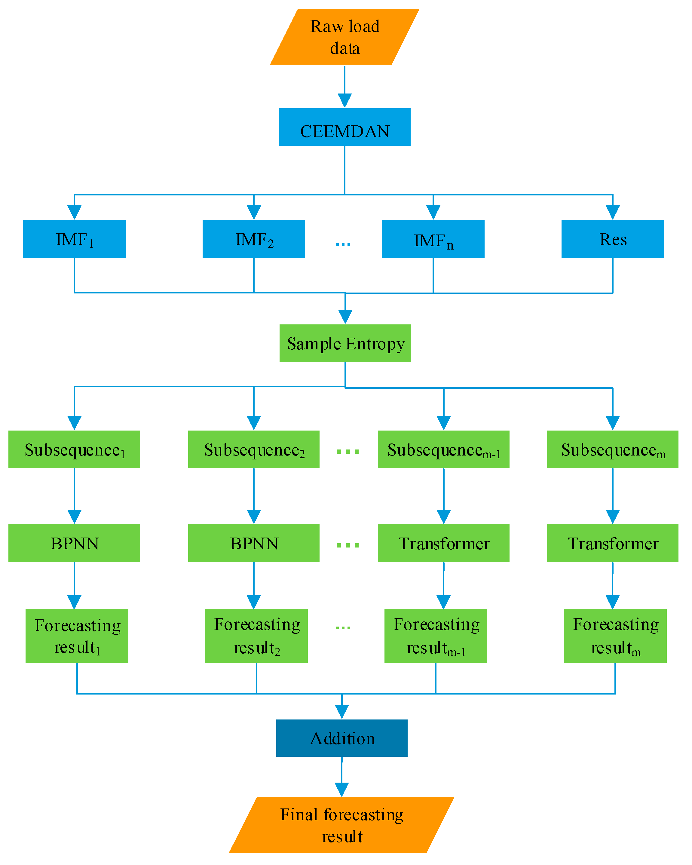
2. Combined Forecasting Model Based on the CEEMDAN-SE-SE-BPNN-Transformer

This paper combined the data decomposition algorithm with the BPNN and the Transformer model, and proposed a combined forecasting model based on the CEEMDAN-SE-BPNN-Transformer. The CEEMDAN-SE was used to decompose the power load into a series of subsequences with obvious differences in complexity, and then the BPNN and the Transformer model were used to model and forecast the subsequences with low and high complexity, respectively. The sequence forecast results were superimposed to obtain the final load forecast results. The flowchart of the proposed algorithm is shown in Figure 1.

Since the power load was affected by many factors, it was difficult for a single forecasting method to obtain accurate forecasting results. Therefore, the CEEMDAN algorithm was used to transform the nonlinear non-stationary time series forecasting problem into several stationary time series forecasting problems, and the complex power load was decomposed into a relatively simple sub-series. At the same time, the SE was used to analyze the complexity of the decomposed stationary subsequences, and it was recombined to form some new subsequences, thereby reducing the amount of calculation and the complexity of the model. For subsequences with higher complexity, the Transformer model based on the attention mechanism can pay more attention, dig out the rules to the greatest extent, and obtain more accurate forecasting results; for subsequences with lower complexity, its periodicity is strong, so a simple-structured BPNN was used for forecast, thereby reducing the training time and avoiding the problem of consuming more resources.

3. Methods

3.1. Complete Ensemble Empirical Mode Decomposition with Adaptive Noise (CEEMDAN)

The Complete Ensemble Empirical Mode Decomposition with Adaptive Noise (CEEMDAN), as an improved method of EMD [15], overcomes the modal aliasing phenomenon of EMD, and also solves the problem of the white noise added in EEMD processing being difficult to remove, and its reconstruction error is very small. The main improvement of CEEMDAN is to add adaptive white noise to the original signal, use EMD to decompose, and average the decomposed components to obtain the final intrinsic mode functions (IMF). The steps of the CEEMDAN algorithm are as follows [20]:

Step 1: Add multiple positive and negative white noises to the original power load sequence x(t). The sequence after adding white noise is as follows:

$$x_{\tau }^{+}\left(t)=x\right(t)+n_{{}_{\tau }}^{+}(t)$$

(1)

$$x_{\tau }^{-}\left(t)=x\right(t)+n_{\tau }^{-}(t)$$

(2)

where, x(t) is the sequence of original power load, $n_{\tau }^{+}$(t) and $n_{\tau }^{-}$(t) are the positive and negative white noise added for the τ-th time.

Step 2: Use the EMD algorithm to perform A times of modal decomposition on the two new sequences $x_{\tau }^{+}$(t) and $x_{\tau }^{-}$(t), and calculate the mean of the two components separately as follows:

$$f^{-}=\frac{1}{A}{\displaystyle \sum _{\tau =1}^A{x}_{\tau }^{-}}$$

(3)

$$f^{+}=\frac{1}{A}{\displaystyle \sum _{\tau =1}^A{x}_{\tau }^{+}}$$

(4)

Step 3: Take the mean of the above two components to obtain the final decomposition result. The steps of CEEMDAN can be summarized as follows:

$$\mathrm{x}(t)={\displaystyle \sum _{i=1}^B{f}_i(t)}+r(t)$$

(5)

3.2. Sample Entropy (SE)

Approximate entropy can measure the complexity of a sequence and only needs a small part of data in a sequence to obtain a result. However, approximate entropy has the disadvantages of poor consistency and easy deviation of calculated results. Therefore, in view of the shortcomings of approximate entropy, Richman [21] proposed the sample entropy theory in 2000. Compared with approximate entropy, sample entropy had better accuracy. The value of the sample entropy directly reflected the complexity of the sequence. The larger the sample entropy value, the more complex the sequence was, and vice versa. The sample entropy is represented by SE(n,α,K), and it can be described as follows [22]:

$$SE(n,\alpha )=\underset{K\to \infty }{\lim }\{-\ln (\frac{R^{n+1}(\alpha )}{R^n(\alpha )})\}$$

(6)

where, K is the length of the time series, n is the dimension, α is the similar tolerance, and Rⁿ⁺¹(α) and Rⁿ(α) are the probability of the two time series matching n or n + 1 points at the threshold value of α. When K takes a finite value, the estimated sample entropy obtained by Equation (6) is:

$$SE(n,\alpha ,K)=-\ln [\frac{R^{n+1}(\alpha )}{R^n(\alpha )}]$$

(7)

3.3. Back Propagation Neural Network (BPNN)

Back Propagation Neural Network (BPNN) [23] is a widely used forecasting method with simple structure and good generalization performance. Compared with SVR and Autoregressive Integrated Moving Average model (ARIMA), it can more accurately forecast the load with strong periodicity and smoothness. Therefore, BPNN is selected in this paper to forecast the subsequence with low complexity.

3.4. Transformer Model

For subsequences with high complexity, BPNN cannot obtain accurate forecasting results due to its simple structure, while the Transformer model based on an attention mechanism [24] has strong feature extraction ability and good fitting ability for subsequences with high complexity. For the time series with high complexity, the Transformer model will pay more attention, that is, compared with the time series with low complexity, the time series with high complexity will gain higher attention weight in the Transformer model, so the forecasting results will be more accurate. Therefore, this paper adopted the Transformer model to forecast the subsequences with high complexity of load.

In 2017, the Google team put forward a model completely based on an Attention-Transformer [24], which consisted of two parts: encoder and decoder. Its structure was more complex than Attention, and the Transformer model was widely used in various fields, such as natural language processing (NLP), machine translation, time series forecasting [25], question answering systems, text summarization, and speech recognition. The structure of the Transformer model [25] is shown in Figure 2.

The Transformer model adopted in this paper is composed of encoder-decoder structure. The Transformer model introduced an attention mechanism in the encoder and decoder in order to have better feature extraction effects. The input layer mapped the input time series data into a d_model dimensional vector through a fully connected network, and encoded sequential information in time series data by adding the input vector element-wise to the positional encoding vector by using position encoding with sine and cosine functions. The resulting vectors were fed into six encoder layers. Each encoder layer consisted of two sublayers: a self-attention sublayer and a fully-connected feed-forward sub-layer. To build a deeper model, residual connections were applied to each sub-layer, followed by a layer normalization. The encoder generated a d_model dimensional vector to feed to the decoder. The decoder used a decoder design similar to the structure of the original Transformer model [24]. The decoder consisted of an input layer, six identical decoder layers, and an output layer.

The Transformer model used a self-attention mechanism to learn the long-term relationship of different time steps [26]. The introduction of the attention mechanism was to solve the problem of information loss caused by too long information. Among them, the attention mechanism obtains the values V ∈ R^N×dV according to the keys K ∈ R^N×dattn and the queries Q ∈ R^N×dattn, as shown in the following equation:

$$\mathit{Q}=\mathit{X}{\mathit{W}}_Q$$

(8)

$$\mathit{K}=\mathit{X}{\mathit{W}}_K$$

(9)

$$\mathit{V}=\mathit{X}{\mathit{W}}_V$$

(10)

$$\mathrm{Attention}(\mathit{Q},\mathit{K},\mathit{V})=A(\mathit{Q},\mathit{K})\mathit{V}$$

(11)

where, X is the input sequence, W_Q, W_K, and W_V are the initialized queries, keys, and values, and A() is the normalization function in Formula (11), which can be expressed as follows:

$$A(\mathit{Q},\mathit{K})=\mathrm{Softmax}(\mathit{Q}{\mathit{K}}^T/\sqrt{d_{attn}})$$

(12)

In order to improve the learning ability of the standard attention mechanism, a multi-head attention mechanism was proposed in [23], which used different heads to represent the subspaces, as shown in Equation (13):

$$MultiHead(\mathit{Q},\mathit{K},\mathit{V})=[{\mathit{H}}_1,...,{\mathit{H}}_{mH}]{\mathit{W}}_H$$

(13)

$${\mathit{H}}_h=\mathrm{Attention}(\mathit{Q}{\mathit{W}}_Q{}^{(h)},\mathit{K}{\mathit{W}}_K{}^{(h)},\mathit{V}{\mathit{W}}_V{}^{(h)})$$

(14)

where, ${\mathit{W}}_K^{\left(h\right)}$∈ R^{dmodel×dattn}, ${\mathit{W}}_Q^{\left(h\right)}$∈ R^{dmodel×dattn}, ${\mathit{W}}_V^{\left(h\right)}$∈ R^dmodel×dv are parameter matrices for keys, queries, and values.

The Transformer model used the attention mechanism to mine the inherent laws of subsequences with high complexity, so that it can more accurately fit the subsequences with high complexity, realize accurate forecast of subsequences with high complexity, and improve the forecasting accuracy of load.

4. Experiments and Discussion

The commonly used evaluation indexes, MAPE and RMSE, were used to compare the forecasting results obtained by the algorithm proposed in this paper (CEEMDAN-SE-BPNN-Transformer) with Transformer, GRU, EEMD-SE-BPNN-Transformer, EEMD-GRU-MLR, CEEMDAN-SE-BPNN-GRU, and CEEMDAN-SE-BPNN-Transformer (unrecombined) algorithms, to prove the superiority of the proposed method in this paper.

4.1. Data Standardization

In order to better extract the internal characteristics of load data, z-score standardization is used to process the data. Its calculation formula is as follows:

$$x_N=\frac{x-x_M}{x_{std}}$$

(15)

where, x_N is the standardized value of load data, x is the value to be standardized of load data, x_M is the mean of the load data, and x_std is the standard deviation of the load data.

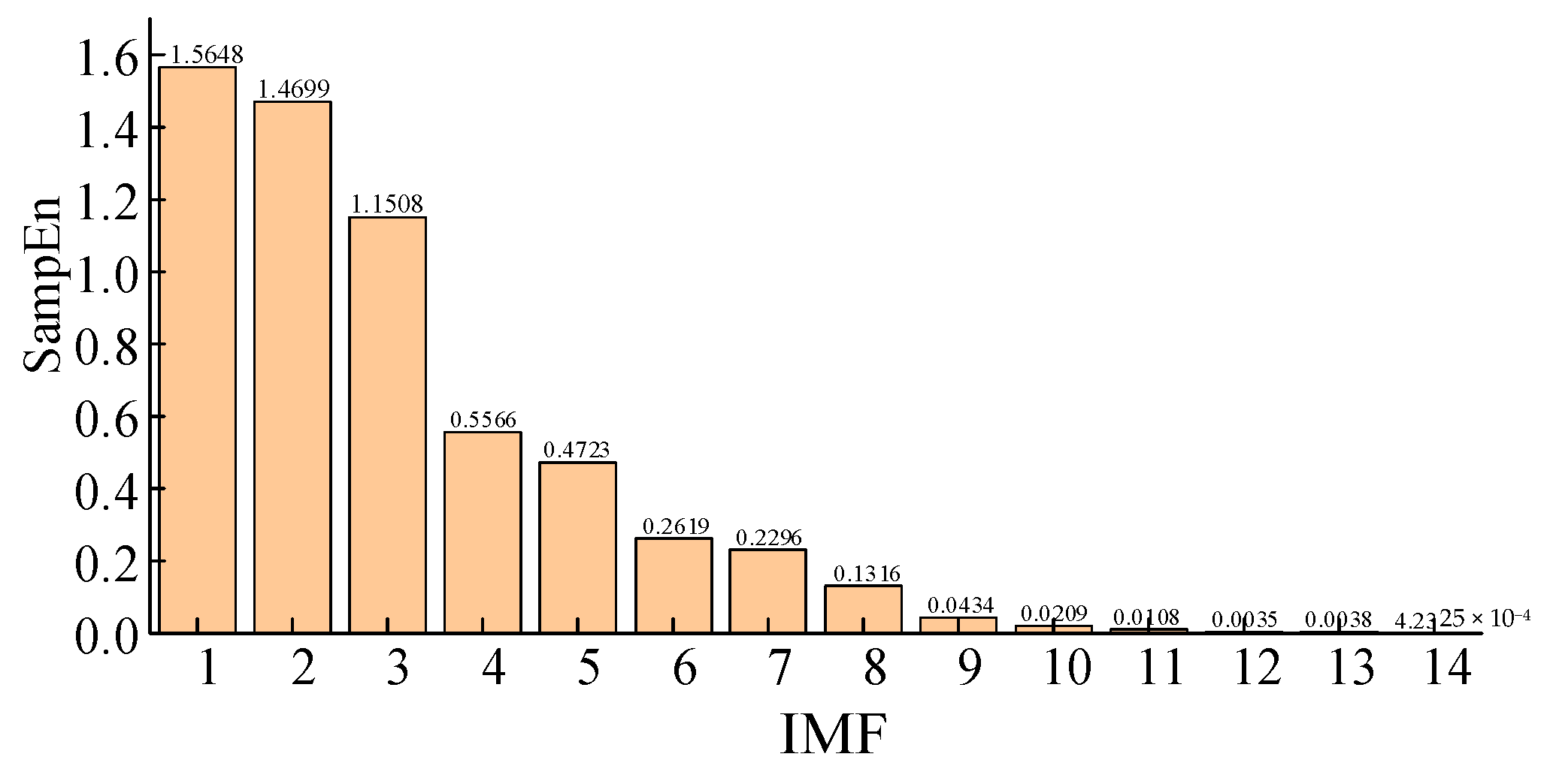
4.2. Power Load Data Decomposition and Complexity Analysis

We used the load data of a certain place in Spain from 1 January to 29 January 2016 as the training set, with a sampling interval of 1 h. The load data from a certain area of Spain was retrieved from https://www.kaggle.com/nicholasjhana/datasets (accessed 20 February 2022). The testing set was the load data of 24 points on 30 January 2016. The load data are shown in Figure 3.

It can be seen from Figure 3 that the original power data have the characteristics of strong randomness, and the ADF test shows that the sequence has a unit root, indicating that the sequence is a non-stationary sequence. Firstly, the standardized load data were decomposed by the CEEMDAN algorithm, and a total of 14 components were obtained from the decomposition. Since there were as many as 14 IMFs obtained by the CEEMDAN decomposition, if each component is directly modeled and forecasted, the amount of calculation will be greatly increased, and the accumulation of excessive component errors will lead to excessive errors in the final forecasting results. Therefore, we used the sample entropy to evaluate the complexity of each decomposed component, and recombined each component according to the value of sample entropy, and then modeled and forecasted the recombined subsequences. The sample entropy of each component is shown in Figure 4.

It can be seen from Figure 4 that the sample entropy of the first eight IMFs were all greater than 0.1, indicating that these eight IMFs were highly complex; the sample entropy of the last six IMFs were all less than 0.1, indicating that these six IMFs were of low complexity. The sample entropy of IMF1, IMF2, and IMF3 were all greater than 1, indicating that the three IMFs had strong randomness. The ample entropy values between the two components IMF1 and IMF2 were close to each other, indicating that the probability of these two IMFs generating a new pattern was roughly the same, so these two components were superimposed to form a new subsequence, and the Transformer model was used to forecast this new sequence. There was a little difference in the sample entropy of IMF4 and IMF5, indicating that the probability of these two IMFs generating a new pattern was roughly the same, so these two IMFs were superimposed to form a new subsequence, and the Transformer model was used to forecast this new sequence. The sample entropy of IMF9 and IMF10 was not much different, and the entropy value was relatively small, so the two IMFs were superimposed into a new subsequence. The sample entropy values of IMF11, IMF12, IMF13, and IMF14 were very close, and the sample entropy values were all less than 0.1. Therefore, IMF11, IMF12, IMF13, and IMF14 were superimposed into a new subsequence.

We forecasted the low-complexity subsequences using BPNN, SVR, and ARIMA, then analyzed the forecasting results. In order to better evaluate the forecast model, this paper adopted the root mean square error (RMSE) and the mean absolute percentage error (MAPE) as the evaluation indexes. The calculation formula of each evaluation index are as follows:

$$e_{RMSE}=\sqrt{\frac{1}{m}{\displaystyle \sum _{k=1}^m[x(k)}-y(k){]}^2}$$

(16)

$$e_{MAPE}=\frac{1}{m}{\displaystyle \sum _{k=1}^m(\frac{\left|x(k)-y(k)\right|}{x(k)}})\times 100\%$$

(17)

where, y(k) and x(k) are the forecasting value and the true value at point k, and m is the total number of samples.

The forecasting accuracy of each model on the low-complexity subsequences are shown in

Table 1. Short-term forecasting performance of BPNN, SVR, and ARIMA on low-complexity subsequences.

Model	BPNN	SVR	ARIMA
RMSE/MW	10.3618	24.3162	34.9004
MAPE/%	0.0305	0.0757	0.1225

.

From Table 1, it can be seen that the MAPE of the BP neural network on the low complexity subsequences was only 0.0305%, the RMSE was only 10.3618 MW, and the two errors were smaller than those of SVR and ARIMA. SVR was difficult to select a suitable kernel function; compared with it, the parameter adjustment of BPNN was relatively simple. Therefore, this showed that BPNN was more suitable for the forecast of subsequences with low complexity, and can accurately obtain the forecasting results.

The recombined results of each IMF and the forecasting models used are shown in

Table 2. Recombined results of each component.

IMF	NEW IMF	Forecasting Model
1, 2	1	Transformer
3	2	Transformer
4, 5	3	Transformer
6, 7, 8	4	Transformer
9, 10	5	BPNN
11, 12, 13, 14	6	BPNN

.

According to the recombined results in Table 2, the subsequences were modeled and forecasted respectively. Finally, the forecasting results of each sub-sequence were superimposed to obtain the final forecasting result of power load.

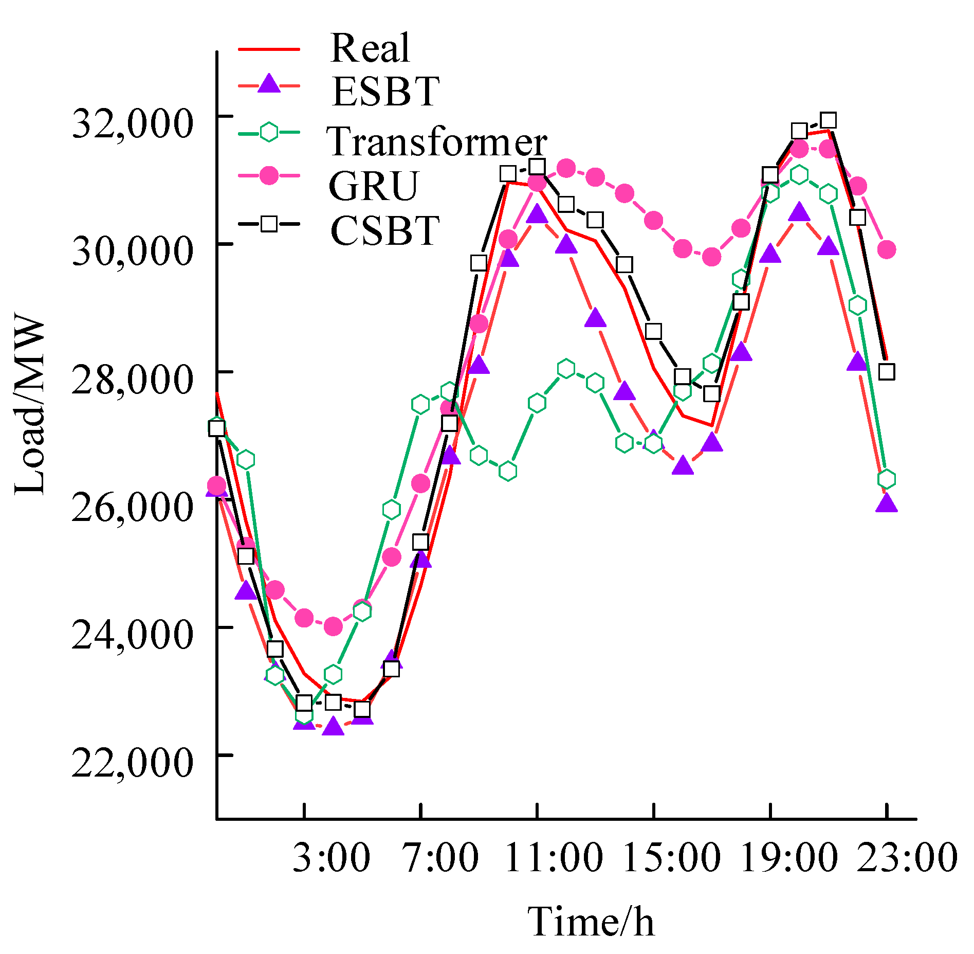
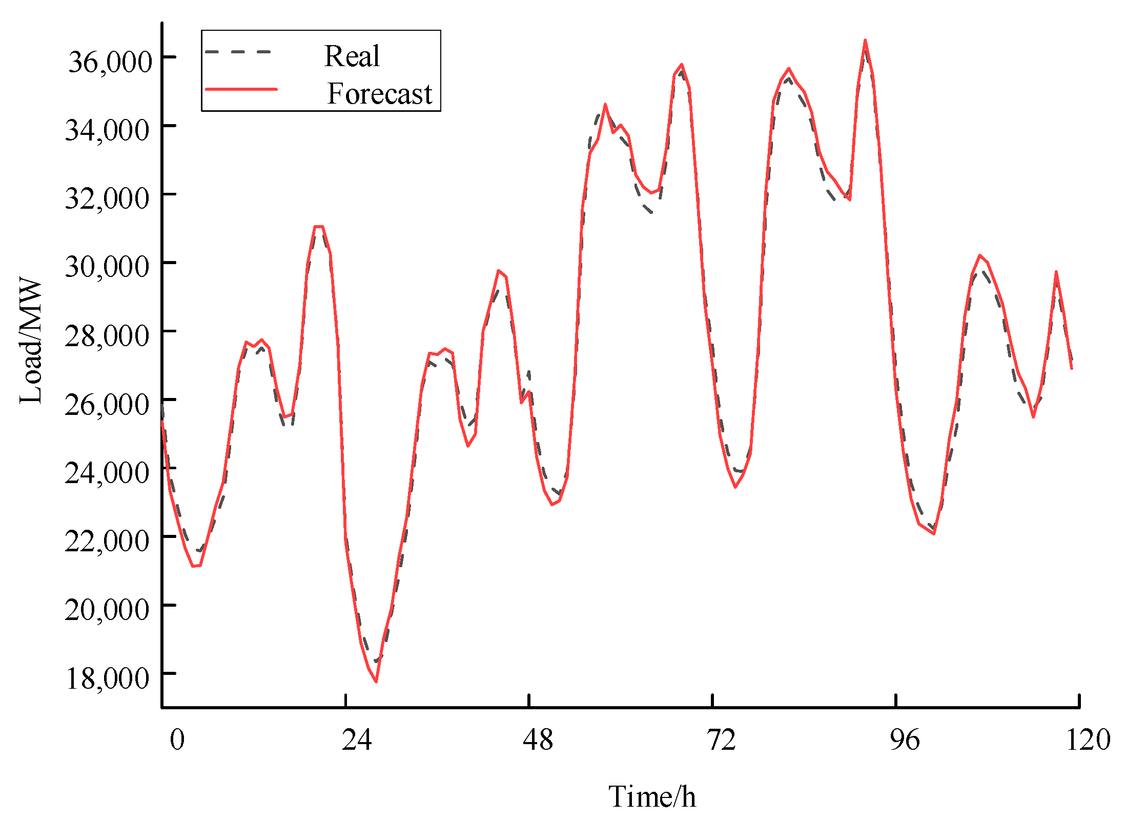
4.3. Comparative Analysis of Forecasting Results

After obtaining the forecasting results of the recombined subsequences, the final power load forecasting value was obtained by adding the forecasting results. The forecasting results are shown in Figure 5 and Figure 6. In order to demonstrate the superiority of the sample entropy-BPNN-Transformer, CSBT was compared with other several forecasting methods. In order to achieve the best forecasting effect of the model, the parameters of each subsequence in each model were adjusted according to the characteristics of the load subsequences and the forecasting condition during the forecasting process. The forecasting methods for comparison are shown below:

(1)

Load forecasting using the Transformer model.

(2)

Load forecasting using GRU model.

(3)

Use the EEMD algorithm to decompose the original load, and then use the sample entropy to analyze the complexity and recombine the components, and then use the BPNN and the Transformer model to forecast the subsequences with low complexity and the subsequences with high complexity, respectively, abbreviated as ESBT.

(4)

Use the EEMD algorithm to decompose the original load, and use the zero-crossing rate proposed in [13], as the basis for dividing high-frequency components and low-frequency components, and divide the decomposed sequence into high-frequency parts and low-frequency parts, then MLR and GRU are used to forecast the low-frequency parts and the high-frequency parts, respectively, abbreviated as EGM.

(5)

Use the CEEMDAN algorithm to decompose the original load, and then use the sample entropy to analyze the complexity and recombine the components, and then use the BPNN and the GRU model to forecast the subsequences with low complexity and the subsequences with high complexity, abbreviated as CSBG.

(6)

Use the CEEMDAN algorithm to decompose the power load data, and then use the sample entropy to analyze the complexity, and divide the components into subsequences with low complexity and high complexity, and then the BPNN and Transformer model are used to forecast the low complexity subsequences and high complexity subsequences, respectively, abbreviated as CSBT (unrecombined).

The detailed settings for BPNN tuning parameters are shown in

Table 3. The adopted parameters of BPNN.

Tuning Parameters	Values
Number of layers	4
Number of hidden layers	2
Activation function	Sigmoid
Learning Rate	0.0001

.

The detailed settings for the Transformer model’s tuning parameters are shown in

Table 4. The adopted parameters of the Transformer model.

Tuning Parameters	Values
Learning rate	0.0001
Dropout	0.1
Batch size	24
dmodel	256
Number of encoder layers	6
Number of decoder layers	6
Number of multi-head attention	8

.

The comparison between the forecasting results of the proposed method, CSBT, and the three methods of Transformer, GRU, and ESBT is shown in Figure 5. The forecasting errors of the model proposed in this paper and several other comparative models are shown in

Table 5. Comparison of forecasting errors of each model.

Model	RMSE/MW	MAPE (%)
GRU	1857.99	5.4547
Transformer	1334.25	4.1312
EGM	1137.11	3.4130
ESBT	936.66	2.9513
CSBG	803.68	2.3840
CSBT (unrecombined)	412.60	1.2958
CSBT	304.40	1.1317

.

As can be seen from Figure 5, compared with the three methods of Transformer, GRU, and ESBT, the forecasting results of the proposed method was closer to the real load curve, and accurate forecasting results were obtained at the positions of the peaks and troughs. Compared with the two single forecasting methods of Transformer and GRU, the results obtained by the ESBT model were closer to the real values. ESBT used EEMD-sample entropy to decompose the data into several subsequences with low complexity and high complexity, and fully excavated the internal features of data. However, the white noise added by EEMD method during decomposition was difficult to remove. As a result, the reconstruction error was too large, therefore, the forecasting result error was too large. The method proposed in this paper used the CEEMDAN method to decompose data, with small reconstruction error and high accuracy of the final forecasting results.

As shown in Table 5, the RMSE of the proposed method in this paper was only 304.40 MW, which was 632.26 MW, 1029.85 MW, and 1553.59 MW less than ESBT, Transformer, and GRU methods, respectively. In addition, compared with the MAPE of ESBT, Transformer, and GRU, the MAPE of the proposed method was only 1.1317%. Therefore, compared with a single algorithm, the method of data decomposition and then forecast in this paper can effectively extract load data features and obtain more accurate forecasting results. This reflects the effectiveness of load decomposition in improving forecasting accuracy, and overcomes the defect that a single algorithm cannot effectively extract load features.

The comparison between the forecasting results of the method proposed in this paper (CSBT) and the three combined forecasting methods of EGM, CSBG, and CSBT (unrecombined) is shown in Figure 6.

As shown in Figure 6, the forecasting results of the proposed model (CSBT) and the CSBT (unrecombined) method are more consistent with the real load data. The other two forecasting methods, EGM and CSBG, had generally obtained good forecasting results, but the error between the forecasting results of these two methods and the real load value was relatively large in some peaks and troughs. During the period from 3:00 to 7:00, as shown in Figure 6, the power load was in a trough state, and the method proposed in this paper (CSBT) can better forecast the change trend, while the forecasting results of the CSBG model and EGM model obviously had a large error with the actual load value. From the perspective of forecasting error, the RMSE of the method proposed in this paper was only 304.40 MW, and compared with the EGM and CSBG models, the RMSE was reduced by 832.71 MW and 499.28 MW, respectively. The MAPE of the EGM method was 3.4130%, the MAPE of the CSBG method was 2.3840%, and the MAPE of the method proposed in this paper was only 1.1317%. The proposed method in this paper chose the Transformer model to forecast the subsequences with high complexity, and it was seen that after decomposing the load data, compared with using GRU to forecast the subsequences with higher complexity, the Transformer model can learn its inherent law more deeply, extract its features in depth, and obtain accurate forecasting results. In addition, CEEMDAN is used for data decomposition in the forecasting method proposed in this paper, and its reconstruction error was small, therefore, the final forecasting result had high accuracy. In this paper, the sample entropy is used to evaluate the complexity of the IMFs, and the IMFs were recombined according to the entropy value to obtain 6 subsequences, and the 6 subsequences were modeled and forecasted, respectively. Compared with the direct forecasting of the 14 IMFs obtained by decomposition, 8 forecasting models were reduced, and the calculation scale was reduced while ensuring relatively high forecasting accuracy.

In order to further prove the superiority and effectiveness of the method proposed in this paper, we used the proposed method to forecast the load from 31 January 2016 to 4 February 2016 by rolling forecasting. That is, the load from 2 January to 30 January were used as the training data to forecast the load value on 31 January, and the load data from 3 January to 31 January were used as training data to forecast the load value on 1 February. The forecasting value from 31 January to 4 February was also obtained by this way, and the forecasting results are shown in Figure 7.

As shown in Figure 7, the obtained load forecasting result was very close to the real value, and the MAPE from 31 January to 4 February was only 1.17%. It can be seen that the method proposed in this paper had a good stable forecasting effect, and the forecasting accuracy was also high. In summary, the forecasting method proposed in this paper was feasible and can effectively improve the forecasting accuracy.

5. Conclusions

A short-term load forecasting model based on the CEEMDAN-SE-BPNN-Transformer is proposed in this paper. Through the example simulation, it was demonstrated that the proposed method not only overcame the shortcomings regarding a single model which cannot effectively extract the characteristics of load data, but that it also improved the forecasting accuracy effectively.

In order to improve the accuracy of short-term load forecasting, a combined forecasting method was proposed based on the CEEMDAN, SE, BPNN, and Transformer model. The CEEMDAN algorithm was used to transform the nonlinear non-stationary time series forecasting problem into several stationary time series forecasting problems, and the complex power load was decomposed into a relatively simple sub-series. At the same time, the SE was used to analyze the complexity of the decomposed stationary subsequences, and it was recombined to form some new subsequences, thereby reducing the amount of calculation and the complexity of the model. For subsequences with higher complexity, the Transformer model based on the attention mechanism paid more attention, dug out the rules to the greatest extent, and obtained more accurate forecasting results; for subsequences with lower complexity, its periodicity was strong, therefore, a simple-structured BPNN was used for forecasting, thereby reducing the training time and avoiding the problem of consuming more resources. The simulation results indicated that the CEEMDAN-SE-BPNN-Transformer forecasting model had a MAPE of 1.1317%, and an RMSE of 304.40, with an overall better forecasting performance than the comparative models.

References

1. Tan, Z.; Zhang, J.; He, Y.; Zhang, Y.; Xiong, G.; Liu, Y. Short-term load forecasting based on integration of SVR and stacking. IEEE Access 2020, 8, 227719–227728. [Google Scholar] [CrossRef]
2. Mishra, M.; Nayak, J.; Naik, B.; Abraham, A. Deep learning in electrical utility industry: A comprehensive review of a decade of research. Eng. Appl. Artif. Intell. 2020, 96, 104000. [Google Scholar] [CrossRef]
3. Li, B.; Lu, M. Short-term load forecasting modeling of regional power grid considering real-time meteorological coupling effect. Autom. Electr. Power Syst. 2020, 44, 60–68. [Google Scholar]
4. Lu, J.; Zhang, Q.; Yang, Z.; Tu, M.; Lu, J.; Peng, H. Short-term load forecasting method based on hybrid CNN-LSTM neural network model. Autom. Electr. Power Syst. 2019, 43, 131–137. [Google Scholar]
5. Wu, F.; Cattani, C.; Song, W.; Zio, E. Fractional ARIMA with an improved cuckoo search optimization for the efficient Short-term power load forecasting. Alex. Eng. 2020, 59, 3111–3118. [Google Scholar] [CrossRef]
6. Hermias, J.P.; Teknomo, K.; Monje, J.C.N. Short-term stochastic load forecasting using autoregressive integrated moving average models and hidden Markov model. In Proceedings of the International Conference on Information and Communication Technologies, Karachi, Pakistan, 26–28 September 2018; pp. 131–137. [Google Scholar]
7. Hong, W.-C.; Fan, G.-F. Hybrid Empirical Mode Decomposition with Support Vector Regression Model for Short Term Load Forecasting. Energies 2019, 12, 1093. [Google Scholar] [CrossRef] [Green Version]
8. Rendon-Sanchez, J.F.; de Menezes, L.M. Structural combination of seasonal exponential smoothing forecasts applied to load forecasting. Eur. J. Oper. Res. 2019, 275, 916–924. [Google Scholar] [CrossRef]
9. Fan, G.-F.; Yu, M.; Dong, S.-Q.; Yeh, Y.-H.; Hong, W.-C. Forecasting short-term electricity load using hybrid support vector regression with grey catastrophe and random forest modeling. Util. Policy 2021, 73, 101294. [Google Scholar] [CrossRef]
10. Zhang, Y.; Ai, Q.; Lin, L.; Yuan, S.; Li, S. A very short-term load forecasting method based on deep LSTM at zone level. Power Syst. Technol. 2019, 43, 1884–1892. [Google Scholar]
11. Jin, Y.; Guo, H.; Wang, J.; Song, A. A Hybrid System Based on LSTM for Short-Term Power Load Forecasting. Energies 2020, 13, 6241. [Google Scholar] [CrossRef]
12. Jin, Y.; Guo, H.; Wang, J.; Song, A. Deep learning methods and applications for electrical power systems: A comprehensive review. Int. J. Energy Res. 2020, 44, 7136–7157. [Google Scholar]
13. Deng, D.; Li, J.; Zhang, Z. Short-term electric load forecasting based on EEMD-GRU-MLR. Power Syst. Technol. 2020, 44, 593–602. [Google Scholar]
14. Chen, Z.; Liu, J.; Li, C. Ultra short-term power load forecasting based on combined LSTM-XGBoost model. Power Syst. Technol. 2020, 44, 614–620. [Google Scholar]
15. Gao, X.; Li, X.; Zhao, B.; Ji, W.; Jing, X.; He, Y. Short-Term Electricity Load Forecasting Model Based on EMD-GRU with Feature Selection. Energies 2019, 12, 1140. [Google Scholar] [CrossRef] [Green Version]
16. Li, B.; Zhang, J.; He, Y.; Wang, Y. Short-term Load forecasting method vased on wavelet decomposition with second-order gray neural network model combined with ADF test. IEEE Access 2017, 05, 16324–16331. [Google Scholar] [CrossRef]
17. Peng, P.; Liu, M. Short-term load forecasting method based on Prophet-LSTM combined model. Proc. CSU-EPSA 2021, 33, 15–20. [Google Scholar]
18. Li, J.; Zhou, S.; Li, H. Short-term electricity forecasting method based on GRU and STL decomposition. J. Shanghai Univ. Electr. Power 2020, 36, 415–420. [Google Scholar]
19. Lei, B.; Wang, Z. Research on short-term load forecasting method based on EEMD-CS-LSSVM. Proc. CSU-EPSA 2019, 33, 117–122. [Google Scholar]
20. Chen, J.; Hu, Z.; Chen, W. Load prediction of integrated energy system based on combination of quadratic modal decomposition and deep bidirectional long short-term memory and multiple linear regression. Autom. Electr. Syst. 2021, 45, 85–94. [Google Scholar]
21. Richman, J.S.; Moorman, J.R. Physiological time-series analysis using approximate entropy and sample entropy. Am. J. Physiol. Heart Circ. Physiol. 2000, 278, 2039–2049. [Google Scholar] [CrossRef] [Green Version]
22. Jia, S.; Ma, B.; Guo, W.; Li, Z.S. A sample entropy based prognostics method for lithium-ion batteries using relevance vector machine. J. Manuf. Syst. 2021, 61, 773–781. [Google Scholar] [CrossRef]
23. Hu, Y.; Li, J.; Hong, M.; Ren, J. Short term electric load forecasting model and its verification for process industrial enterprises based on hybrid GA-PSO-BPNN algorithm—A case study of papermaking process. Energy 2019, 170, 1215–1227. [Google Scholar] [CrossRef]
24. Vaswani, A. Attention is all you need. In Proceedings of the 31st International Conference on Neural Information Processing Systems, Long Beach, CA, USA, 4–9 December 2017; pp. 6000–6010. [Google Scholar]
25. Wu, N.; Green, B.; Ben, X.; O’Banion, S. Deep TransformerModels for Times Series Forecasting: The Influenza Prevealence Case. arXiv 2020, arXiv:2001.08317v1. [Google Scholar]
26. Lim, B.; Arik, S.O.; Loeff, N.; Pfister, T. Temporal Fusion Transformers for interpretable multi-horizon time series forecasting. Int. J. Forecast. 2021, 37, 1748–1764. [Google Scholar] [CrossRef]
Figure 1. The flowchart of the CEEMDAN-SE-BPNN-Transformer Model.
Energies 15 03659 g001
Figure 2. The structure of the Transformer Model.
Energies 15 03659 g002
Figure 3. The raw data of power load.
Energies 15 03659 g003
Figure 4. Sample entropy of each component.
Energies 15 03659 g004
Figure 5. The forecasting results of the CBST model, Transformer, GRU, and ESBT model.
Energies 15 03659 g005
Figure 6. The forecasting results of the CBST model, EGM, CSBG, and CSBT (unrecombined) models.
Energies 15 03659 g006
Figure 7. Forecasting results from January 31 to February 4.
Energies 15 03659 g007