Source-Load Coordinated Low-Carbon Economic Dispatch of Electric-Gas Integrated Energy System Based on Carbon Emission Flow Theory

Abstract

The development of emerging technologies has enhanced the demand response (DR) capability of conventional loads. To study the effect of DR on the reduction in carbon emissions in an integrated energy system (IES), a two-stage low-carbon economic dispatch model based on the carbon emission flow (CEF) theory was proposed in this study. In the first stage, the energy supply cost was taken as the objective function for economic dispatch, and the actual carbon emissions of each energy hub (EH) were calculated based on the CEF theory. In the second stage, a low-carbon DR optimization was performed with the objective function of the load-side carbon trading cost. Then, based on the modified IEEE 39-bus power system/Belgian 20-node natural gas system, MATLAB/Gurobi was used for the simulation analysis in three scenarios. The results showed that the proposed model could effectively promote the system to reduce the load peak-to-valley difference, enhance the ability to consume wind power, and reduce the carbon emissions and carbon trading cost. Furthermore, as the wind power penetration rate increased from 20% to 80%, the carbon reduction effect basically remained stable. Therefore, with the growth of renewable energy, the proposed model can still effectively reduce carbon emissions.

1. Introduction

Emissions of greenhouse gases such as carbon dioxide produced by the development of human society have exceeded the capacity of the Earth, causing the greenhouse effect to become increasingly apparent [1,2]. Energy systems are a major source of carbon emissions [3]. Under the Sustainable Development Goals (SDGs), energy systems are in urgent need of low-carbon development [4,5,6]. Integrated energy systems (IESs) have a prominent low-carbon emission potential, attracting a large number of domestic and foreign scholars to conduct relevant research [7,8]. The research on low-carbon IESs has become a hotspot in the international energy field [3,9].

So, how can we effectively mitigate the carbon emissions in IESs? The recent research [10] systematically combs through carbon emission mitigation strategies from the aspects of policies, sector specific technologies and initiatives, and general societal initiatives. Specifically for integrated energy systems, carbon reduction strategies can be roughly divided into two categories: system internal strategies and policy incentive strategies. The internal strategies include developing renewable energy power generation technologies to replace fossil fuel power generation technology, developing energy storage technology to promote renewable energy consumption, optimizing operation strategies to improve energy utilization, developing carbon capture and utilization storage technology, and so on [10,11]. Policy incentive strategies include the use of a carbon tax, carbon trading, time-of-use energy pricing, and other policies to stimulate the energy supply side and consumption side to change toward a direction that is conducive to mitigating carbon emissions [10,12].

Research focusing on the system internal strategies of IESs to reduce carbon emissions have been widely conducted. The study by [13] proposed a day-ahead energy trading strategy for a regional integrated energy system (RIES) that considered energy cascade utilization to improve the energy utilization efficiency. In [14], the concept of a sharing economy was introduced into the energy interaction process of an IES and proposed a distributed electrical–gas–thermal energy sharing mechanism to improve the energy efficiency and promote the optimal resource allocation. The use of power-to-ammonia in high-renewable multi-energy systems is superior to that of regular batteries and power-to-gas storage for system operational economy and renewable energy accommodation [15].

In terms of policy incentive strategies, some studies have focused on the carbon reduction effects of a carbon tax and carbon trading policies on the energy supply side. A carbon tax was introduced into the objective function of the economic dispatch model to improve the system economy and low-carbon performance in [16]. In [17], an economic dispatch model for RIESs was proposed using the ladder carbon prices. The reward and punishment ladder-type carbon trading mechanism was used to calculate the carbon trading cost of an IES considering the carbon capture technology in [9].

On the other hand, some studies have mainly focused on the policy impact on the energy consumption side. Stimulating demand response (DR) through policies is an effective way to increase the renewable energy consumption and reduce the system carbon emissions [18]. The study in [19] used the time-of-use electricity and gas prices to drive the integrated demand response to reduce the system carbon emissions. In [20], they studied the effect of the time-of-use electricity pricing policy on smart home participation in the power demand response. The authors in [21] studied the impact of the dynamic electricity tariffs on the household’s electricity demand response. Demand response guided by real-time electricity prices has also been studied [22,23]. These studies [19,20,21,22,23] were all from the perspective of energy price policy to stimulate the demand response.

However, in the context of decarbonizing the energy system, the demand response motivated by energy price policies is not straightforward enough. Energy demand is the root cause of carbon emissions in the energy system. The responsibility of the energy demand side for system carbon emissions cannot be ignored. Therefore, it is more direct to guide the demand response through carbon price policies. At present, the demand response under the incentive of user-side carbon trading has not been fully studied, and its carbon reduction effectiveness and advantages remain to be discussed.

To study this problem, the first challenge is to calculate the actual carbon responsibility on the user side. The carbon emission flow (CEF) theory first proposed in [24] solves this problem well. The carbon emission flow theory considering power network losses has also been studied [25]. Furthermore, CEF theory has also been adopted in IESs [3,26], which can allocate the actual carbon emission responsibility from the energy supply side to the demand side.

To sum up, the demand response carbon reduction strategy under the CEF-based user-side carbon trading incentive is worth studying. To study the carbon reduction effect of the strategy, a two-stage low-carbon economic dispatch model was proposed in this paper. The main contributions of this paper are as follows:

• This paper proposes a two-stage low-carbon economic dispatch model of the IES based on the CEF theory. On the basis of considering the load-side carbon responsibility and demand response, the source and load are coordinately optimized to realize the low-carbon economic operation of the IES;
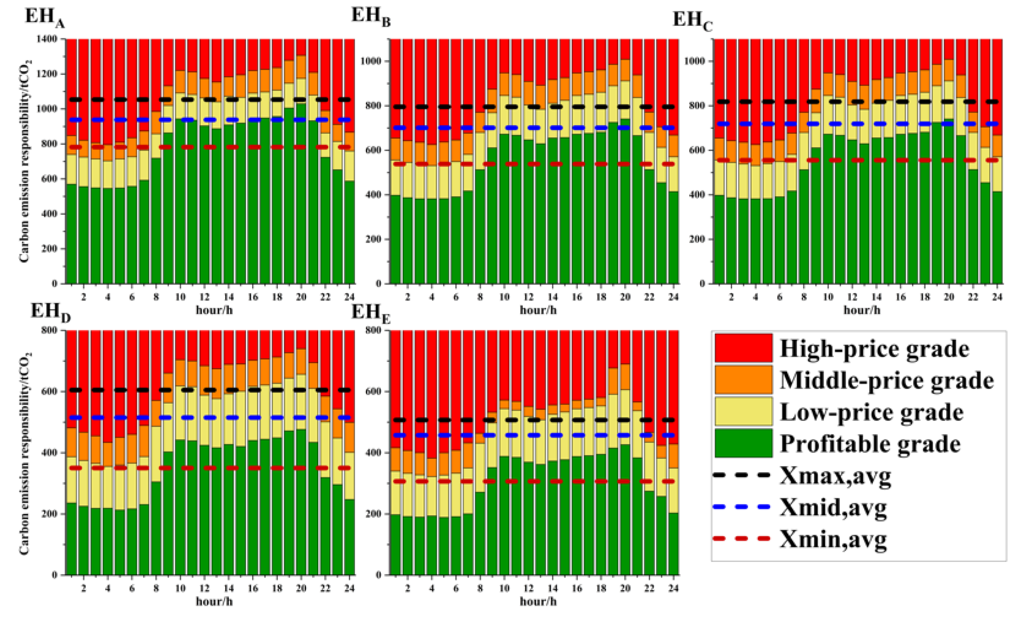
• Based on the Shapley value method, a method for the division of the carbon emission responsibility grades of each energy hub is proposed, and a ladder-type carbon trading mechanism is formulated;
• Through the analysis of three scenarios, the effectiveness of the model proposed in this paper is verified in the IESs with different renewable energy penetration rates, and the mechanism of the demand response is elaborated. Furthermore, the proposed method is proven to have superiority over the other two related existing methods in carbon reduction.

2. Load-Side Carbon Responsibility Allocation Method Based on Carbon Emission Flow Theory and Shapley Value Method

The structure of an electric-gas IES is shown in Figure 1. The solid blue lines represent the power flow from the power source to the load through the power grid. The solid green lines indicate that natural gas flows from the gas source to the gas load through the natural gas network. Electricity and natural gas loads form energy hubs [27]. The blue and green dotted lines in Figure 1 represent the carbon emission flows of electricity and natural gas, respectively. To clarify the carbon emission responsibility that each EH should undertake in the process of using power and natural gas, calculations and analyses can be carried out based on the CEF theory [26]. Subsequently, based on the Shapley value method, the carbon emission responsibility for each EH can be divided into several grades. As a result, a ladder-type carbon-trading mechanism can be formed.

2.1. CEF in Power System Considering Grid Losses

The power system grid loss rate can reach 7–9% [28], and therefore, the carbon emissions caused by grid losses cannot be ignored. Therefore, the carbon emission responsibility caused by grid losses must be attributed to the load side by the CEF considering the grid losses. According to the method introduced in [29], the power flux of bus $i$ is defined as

$$P_{Bi}={\displaystyle \sum }_{j\in i^{+}}{P}_{ji}+P_{Gi}$$

(1)

where $P_{ji}$ is the active power at the end of branch $j-i$, and the positive direction is from $j$ to $i$; $i^{+}$ represents the set of start buses of the branches where the power flows injected into bus $i$ are located; $P_{Gi}$ is the generator output at bus $i$. Equation (2) can be derived from Equation (1):

$${\mathit{P}}_B={\left({\mathit{E}}^{\mathit{g}\mathit{r}\mathit{o}\mathit{s}\mathit{s}}-{\mathit{A}}^{\mathit{g}\mathit{r}\mathit{o}\mathit{s}\mathit{s}}\right)}^{-1}{\mathit{P}}_G$$

(2)

where ${\mathit{P}}_B$ is an $n$-dimensional column vector representing the power fluxes of buses for a power grid with $n$ buses; ${\mathit{E}}^{\mathit{g}\mathit{r}\mathit{o}\mathit{s}\mathit{s}}$ is an $n$-order identity matrix; ${\mathit{A}}^{\mathit{g}\mathit{r}\mathit{o}\mathit{s}\mathit{s}}$ is an $n\times n$ coefficient matrix, each element of which is defined as

$${\mathit{A}}_{ij}^{gross}=\{\begin{array}{c}{P}_{ji}^{gross}/P_{Bj} j\in i^{+}\\ 0 else\end{array}$$

(3)

where $P_{ij}^{gross}$ is the active power at the start of branch $j-i$, which is defined as $P_{ij}^{gross}=P_{ji}+P_{ij}^{loss}$; $P_{ij}^{loss}$ is the grid loss on branch $j-i$. Correspondingly, it can be obtained as:

$${\mathit{P}}_L^{gross}={\mathit{B}}^{\mathit{g}\mathit{r}\mathit{o}\mathit{s}\mathit{s}}{\mathit{P}}_B$$

(4)

where ${\mathit{P}}_L^{gross}$ is an $n$-dimensional column vector, which denotes the equivalent electrical load value after allocating the grid losses to each load, ${\mathit{B}}^{\mathit{g}\mathit{r}\mathit{o}\mathit{s}\mathit{s}}$ is an $n$-order diagonal coefficient matrix, each element of which is defined as

$${\mathit{B}}_{ij}^{gross}=\{\begin{array}{c}{P}_{Li}/P_{Bj} i=j\\ 0 i\ne j\end{array}$$

(5)

From Equations (2) and (5), it can be obtained:

$${\mathit{P}}_L^{gross}={\mathit{B}}^{\mathit{g}\mathit{r}\mathit{o}\mathit{s}\mathit{s}}{\left({\mathit{E}}^{\mathit{g}\mathit{r}\mathit{o}\mathit{s}\mathit{s}}-{\mathit{A}}^{\mathit{g}\mathit{r}\mathit{o}\mathit{s}\mathit{s}}\right)}^{-1}{\mathit{P}}_G={\mathit{T}}^{\mathit{g}\mathit{r}\mathit{o}\mathit{s}\mathit{s}}{\mathit{P}}_G$$

(6)

where ${\mathit{T}}^{\mathit{g}\mathit{r}\mathit{o}\mathit{s}\mathit{s}}$ is the distribution matrix from the source to the load, which can be calculated from the direct current (DC) optimal power flow results considering the grid losses. The element ${\mathit{T}}_{ij}^{gross}$ represents the percentage of generator output at bus $j$ supplied to the load at bus $i$, and therefore the sum of elements in each column of ${\mathit{T}}^{\mathit{g}\mathit{r}\mathit{o}\mathit{s}\mathit{s}}$ is 1.

Because the carbon emission flow is a virtual flow attached to the active power flow, analogous to Equation (2), it can be obtained as:

$${\mathit{R}}_{ele,B}={\left({\mathit{E}}^{\mathit{g}\mathit{r}\mathit{o}\mathit{s}\mathit{s}}-{\mathit{A}}^{\mathit{g}\mathit{r}\mathit{o}\mathit{s}\mathit{s}}\right)}^{-1}{\mathit{R}}_G$$

(7)

where ${\mathit{R}}_G$ is an $n$-dimensional column vector representing the carbon flow rate of the generators in $tC{O}_2/h$. The calculation method for the elements is

$$R_{Gi}=e_{Gi}{P}_{Gi}$$

(8)

where $e_{Gi}$ is the carbon emission intensity of the generator at bus $i$, in $tC{O}_2/MWh$.

Analogous to Equation (6), this is:

$${\mathit{R}}_{ele,L}^{gross}={\mathit{T}}^{\mathit{g}\mathit{r}\mathit{o}\mathit{s}\mathit{s}}{\mathit{R}}_G$$

(9)

where ${\mathit{R}}_{ele,L}^{gross}$ is an $n$-dimensional column vector that denotes the load-side carbon emission responsibility after the source-side carbon emissions are attributed to the load side considering grid losses. On this basis, the bus carbon intensity ${\mathit{e}}_{ele}^{gross}$ can be calculated, the unit of which is $tC{O}_2/MWh$. The calculation method for the elements is as follows:

$$e_{ele,i}^{gross}=R_{D,ele,i}^{gross}/P_{Bi}$$

(10)

2.2. CEF in a Natural Gas System

The CEF of an isolated lossless gas system is completely determined by the mass flow. Assuming that the carbon emission intensities of all gas sources are the same, the carbon emission responsibility of the load side can only be calculated directly according to the load value. However, as the carbon intensity of the power-to-gas (P2G) node changes, the carbon intensity of each gas node is no longer constant. Therefore, it is necessary to adopt the CEF theory to calculate the carbon emission responsibility on the gas load side.

In this study, the steady-state modeling of a natural gas system neglecting pipe storage and pipeline losses was adopted; thus, the CEF theory without considering the network losses can be applied. Because the CEF without grid losses is a special case of the CEF in Section 2.1, the following parts can be obtained.

The mass-flow flux $F_{Bi}$ of node $i$ is:

$$F_{Bi}={\displaystyle \sum }_{j\in i^{+}}{F}_{ji}+F_{Si}$$

(11)

where $F_{ji}$ is the gas mass flow rate of pipeline $j-i$, and the positive direction is from $j$ to $i$; $i^{+}$ represents the set of start nodes of the pipelines where the gas flows injected into node $i$ is located; $F_{si}$ is the mass flow rate of the gas source at node $i$. By analogy, it can be obtained as:

$${\mathit{F}}_B={\left(\mathit{E}-\mathit{A}\right)}^{-1}{\mathit{F}}_s$$

(12)

where ${\mathit{F}}_B$ is an $m$-dimensional column vector representing the node mass flow flux for a gas network with $m$ nodes; $\mathit{E}$ is an $m$-order identity matrix; $\mathit{A}$ is an $m\times m$ coefficient matrix, each element of which is defined as

$${\mathit{A}}_{ij}=\{\begin{array}{c}{F}_{ji}/F_{Bj} j\in i^{+}\\ 0 else\end{array}$$

(13)

where $F_{ji}$ is the gas mass flow rate of pipeline $j-i$; correspondingly, which can be obtained as follows:

$${\mathit{F}}_L=\mathit{B}{\left(\mathit{E}-\mathit{A}\right)}^{-1}{\mathit{F}}_s=\mathit{T}{\mathit{F}}_s$$

(14)

where ${\mathit{F}}_L$ is an $m$-dimensional column vector representing the gas load and $\mathit{B}$ is an $m$-order diagonal coefficient matrix. Each element is defined as follows:

$${\mathit{B}}_{ij}=\{\begin{array}{c}{F}_{Di}/F_{Bj} i=j\\ 0 i\ne j\end{array}$$

(15)

where $\mathit{T}$ is the distribution matrix of the gas network from the source to load. For the carbon emission flow rate in the gas network,

$${\mathit{R}}_{gas,B}={\left(\mathit{E}-\mathit{A}\right)}^{-1}{\mathit{R}}_s$$

(16)

where ${\mathit{R}}_s$ is an $m$-dimensional column vector in $tC{O}_2/h$, representing the carbon flow rate of the gas source. The calculation method of the elements is

$$R_{si}=e_{si}{F}_{si}$$

(17)

where $e_{si}$is the carbon emission intensity of the gas source at node $i$, in $tC{O}_2/MBtu$.

$${\mathit{R}}_{gas,L}=\mathit{T}{\mathit{R}}_S$$

(18)

where ${\mathit{R}}_{gas,L}$ is an $m$-dimensional column vector, which represents the carbon emission responsibility on the load side. Correspondingly, the node carbon intensity of the gas network ${\mathit{e}}_{gas}$, in $tC{O}_2/MBtu$, can be calculated as follows:

$$e_{gas,i}=R_{gas,B,i}/F_{Bi}$$

(19)

2.3. Allocation of Carbon Emission Responsibility Based on the Shapley Value Method

The energy hubs in an IES form a natural cooperative game alliance. The total carbon emissions of the IES are a joint responsibility for all EHs. Therefore, the carbon emission responsibility allocation can be regarded as a classic cost allocation problem. Many methods can be used to solve the cost allocation problem. Among them, the Shapley value (SV) method and generalized nucleolus (GN) method are the most widely used because of their unique solutions and good properties. Compared to the GN method, the SV method is superior in terms of equivalence (the mutual influence between any two members is the same) [30]. Hence, this study adopted the SV method to allocate the carbon emission responsibility among the EHs.

The SV method was proposed by Lloyd Shapley in 1953 and emphasizes the marginal effect of each member for different alliances. According to the definition of the Shapley value, the carbon emission responsibility shared by each EH should be the weighted average of all of its marginal effects, which can be expressed as:

$$X_i={\displaystyle \sum }_{S\subseteq N\backslash \left\{i\right\}}\frac{n_s!\left(n_N-n_s-1\right)!}{n_N!}\left[C\left(S\cup \left\{i\right\}\right)-C\left(S\right)\right]$$

(20)

where $n_N$ represents the number of members in the entire alliance $N$; $S$ represents any sub-alliance without the member $i$; $n_s$ represents the number of members in the sub-alliance $S$; $n_s!\left(n_N-n_s-1\right)!/n_N!$ represents the probability of the occurrence of sub-alliance $S$; $C\left(S\right)$ represents the carbon emission responsibility of the sub-alliance $S$; $S\cup \left\{i\right\}$ represents a new alliance formed by incorporating the alliance member $i$ into alliance $S$; $C\left(S\cup \left\{i\right\}\right)-C\left(S\right)$ represents the carbon emission responsibility marginal effects of member $i$ on sub-alliance $S$.

For each member in an alliance with $n_N$ members, it has $2^{n_N-1}$ marginal effects. Hence, the minimum and maximum marginal effects of member $i$ can be defined as $X_{i,min}$, $X_{i,max}$.

$$X_{i,min}=min\left\{C\left(S\cup \left\{i\right\}\right)-C\left(S\right)\right\}$$

(21)

$$X_{i,max}=max{\left\{C\left(S\cup \left\{i\right\}\right)-C\left(S\right)\right\}}_{ }$$

(22)

The Shapley value $X_i$ is the weighted average of all marginal effects and therefore $X_{i,min}<X_i<X_{i,max}$. The Shapley value of the member $i$ is defined as $X_{i,mid}$.

$$X_{i,mid}=X_i$$

(23)

3. A Two-Stage Low-Carbon Economic Dispatch Model Considering Demand Response

3.1. The Two-Stage Model Overview

The two-stage low-carbon economic dispatch model considering the DR was employed to illustrate the source–load interaction coordination. The detailed process of the two-stage model is presented in Figure 2.

This can be divided into four parts:

• Preparatory work: Based on the method proposed in Section 2, the carbon emission responsibility grades of each EH are calculated using the input data. Thus, a ladder-type carbon trading mechanism is formed to calculate the load-side carbon trading cost in the second stage;
• The first stage: An economic dispatch optimization is performed with the objective function of minimizing the energy supply cost. The flow data of the IES are obtained by optimization. These are then passed to the CEF model to calculate the carbon intensity of each load node;
• The second stage: Based on the first stage, this stage is optimized with the objective function of minimizing the carbon trading cost of the load side. The optimal demand response values are obtained after the optimization;
• Loop solution and output: The response values optimized by the second stage cause load changes, and therefore, it is necessary to use the new load values to perform the first-stage economic dispatch calculation. Finally, a two-stage loop calculation is performed until the objective function values of the two stages tend to be stable.

The modeling of the IES and demand-side response in this study was based on the following hypothesis:

• Without considering the impact of the reactive power flow on the system carbon emissions, the DC power flow modeling was adopted for the power system;
• Without considering the pipeline inventory, the steady-state pipeline modeling was adopted for the gas network;
• The demand-side response was based on the premise that the total energy demand for a day remained unchanged;
• Without considering the power or gas load types, the load response ranges are set to constrain the load response capability.

3.2. The First Stage: Economic Dispatch Model

3.2.1. Objective Function

The objective function is established as flows:

$$min{\displaystyle \sum }_{t=0}^T\left({\displaystyle \sum }_{CFU=1}^{N_{CFU}}{c}_{CFU}{P}_{CFU,t}+{\displaystyle \sum }_{wind=1}^{N_{wind}}{c}_{wind}{P}_{wind,t}+{\displaystyle \sum }_{gas=1}^{N_{gas}}{c}_{gas}{F}_{gas,t}\right)$$

(24)

where $c_{CFU}$ represents the power generation cost coefficient of coal-fired units, which is determined by the fuel cost, power generation efficiency, and so on; $c_{wind}$ is the power generation cost coefficient of the wind turbine, which is determined by the operation cost, maintenance cost, and so on; $c_{gas}$ represents the cost coefficient of natural gas; $P_{CFU,t}$ and $P_{wind,t}$ represents the outputs of the coal-fired units and wind turbines at time $t$, respectively; $F_{gas,t}$ denotes the output mass flow rate of the natural gas source at time $t$.

3.2.2. Constraints

(1)

Power system model

To consider the speed and accuracy of the calculation, this study adopted the DC optimal power flow model considering branch losses [31]. The system has the following constraints.

(a)

Unit constraints:

$$P_{CFU,min}\le P_{CFU,t}\le P_{CFU,max}$$

(25)

$$P_{GFU,min}\le P_{GFU,t}\le P_{GFU,max}$$

(26)

$$P_{wind,min}\le P_{wind,t}\le P_{wind,max}$$

(27)

$$P_{GFU,i}={\eta }_{GFU}{F}_{GFU,m}$$

(28)

$$Ram{p}_{CFU,min}\le P_{CFU,t}-P_{CFU,t-1}\le Ram{p}_{CFU,max}$$

(29)

$$Ram{p}_{GFU,min}\le P_{GFU,t}-P_{GFU,t-1}\le Ram{p}_{GFU,max}$$

(30)

where $P_{CFU,max}$ and $P_{CFU,min}$ represent the upper and lower output limits of the coal-fired units; $P_{GFU,max}$ and $P_{GFU,min}$ represent the upper and lower output limits of the gas-fired units, respectively; $P_{wind,max}$ and $P_{wind,min}$ represent the upper and lower output limits of the wind turbines; $P_{CFU,t}$, $P_{GFU,t}$, and $P_{wind,t}$ are the actual outputs of the coal-fired units, gas-fired units, and wind turbines at time $t$, respectively; ${\eta }_{GFU}$ is the power generation efficiency of the gas-fired units; $F_{GFU,m}$ is the mass flow rate of natural gas consumed by the gas-fired unit, respectively; $Ram{p}_{CFU,max}$ and $Ram{p}_{CFU,min}$ represent the upper and lower output limits of the coal-fired units; $Ram{p}_{GFU,max}$ and $Ram{p}_{GFU,min}$ represent the upper and lower output limits of the gas-fired units, respectively.

(b)

Branch constraints:

$$P_{ij,t}=\frac{{\theta }_{ij,t}}{x_{ij}}$$

(31)

$$P_{ij,t}^{loss}=g_{ij}{\theta }_{ij,t}^2$$

(32)

$$P_{ij,min}\le P_{ij}\le P_{ij,max}$$

(33)

where $P_{ij,t}$ and $P_{ij,t}^{loss}$ represent the power flow and branch losses of branch $i-j$ at time $t$, respectively; ${\theta }_{ij,t}$ is the phase angle difference between the two ends of branch $i-j$ at time $t$; $x_{ij}$ and $g_{ij}$ are the reactance and conductance of branch $i-j$; $P_{ij,max}$ and $P_{ij,min}$ are the upper and lower power transmission limits of branch $i-j$.

(c)

Bus constraints

$$P_{CFU,i}+P_{GFU,i}+P_{wind,i}={\displaystyle \sum }_{j\in {\mathsf{\Omega }}_i}{P}_{ij}+{\displaystyle \sum }_{j\in {\mathsf{\Omega }}_i}\frac{1}{2}{P}_{loss,ij}+P_{L,i}+P_{P2G,i}$$

(34)

$$F_{P2G,m}={\eta }_{P2G}{P}_{P2G,i}$$

(35)

$${\theta }_{ij,min}\le {\theta }_{ij,t}\le {\theta }_{ij,max}$$

(36)

$${\theta }_{ref,t}=0$$

(37)

where $P_{CFU,i}$, $P_{GFU,i}$ and $P_{wind,i}$ represent the power injected into bus $i$ from the coal-fired units, gas-fired units, and wind turbines, respectively; $P_{L,i}$ represents the load on bus $i$; ${\mathsf{\Omega }}_i$ represents the set of all buses around bus $i$; $P_{P2G,i}$ represents the power consumed by the P2G equipment on bus $i$; ${\eta }_{P2G}$ is the energy conversion efficiency of P2G; $F_{P2G,m}$ represents the gas mass flow rate supplied by P2G to node $\mathrm{m}$; ${\theta }_{ij,max}$ and ${\theta }_{ij,min}$ represent the upper and lower phase difference limits of branch $i-j$; ${\theta }_{ref,t}$ is the phase angle of the slack bus at time $t$.

(2)

Natural gas system model

The natural gas system adopts the steady-state modeling based on the Weymouth function [32]. The constraints of the natural gas system are as follows.

(a)

Natural gas source constraints:

$$F_{S,m}^{min}\le F_{S,m}\le F_{S,m}^{max}$$

(38)

where $F_{S,m}$ represents the mass flow rate of the gas source at node $m$; $F_{S,m}^{max}$ and $F_{S,m}^{min}$ represent the upper and lower mass flow rate limits of the gas source at node $m$.

(b)

Pipeline constraints:

$$F_{mn}\left|F_{mn}\right|=k_{mn}\left({\pi }_m^2-{\pi }_n^2\right)$$

(39)

$$F_{mn}^{min}\le F_{mn,t}\le F_{mn}^{max}$$

(40)

where $F_{mn,t}$ represents the gas mass flow rate of pipeline $m-n$ at time $t$. $k_{mn}$ is a constant that depends on the length, diameter, and absolute rugosity of the pipe and the gas composition [32]; ${\pi }_m$ and ${\pi }_n$ denote the gas pressure at nodes $m$ and $n$, respectively; $F_{mn}^{max}$ and $F_{mn}^{min}$ are the upper and lower mass flow rate limits of pipeline $m-n$.

(c)

Node constraints:

$$F_{S,m}+F_{P2G,m}={\displaystyle \sum }_{n\in {\mathsf{\Omega }}_m}{F}_{mn}+F_{L,m}+F_{GFU,m}$$

(41)

$${\pi }_m^{min}\le {\pi }_m\le {\pi }_m^{max}$$

(42)

where $F_{L,m}$ represents the gas load at node $m$; ${\pi }_m^{max}$ and ${\pi }_m^{min}$ represent the upper and lower gas pressure limits of node $m$.

3.3. The Second Stage: Demand Response Model

In the second stage, the optimization focus is shifted from the energy supply side to the energy demand side. The demand response is the behavior of the energy demand side actively changing the demand under market incentives to coordinate with the energy supply. To promote low-carbon energy consumption, a demand-response low-carbon optimization model with a ladder-type carbon price is established in the second stage. The ladder-type carbon price was adopted as the incentive signal, and the minimum demand-side carbon trading cost was set as the goal to optimize the response value.

3.3.1. Objective Function

The objective function of the second stage is to minimize the load-side carbon trading cost.

$$min{\displaystyle \sum }_{t=0}^T{\displaystyle \sum }_{i=1}^{N_{EH}}{C}_{i,t}^{CT}$$

(43)

where $C_{i,t}^{CT}$ is the carbon trading cost of the $E{H}_i$ at time $t$; $N_{EH}$ represents the total number of energy hubs; $T$ represents the time period of an optimization, which is 24 h in this paper.

3.3.2. Constraints

(1)

Carbon trading cost constraints:

If EHs equally share the carbon emission responsibility of the entire IES, it is bound to be an unfair and unreasonable solution. To distribute the carbon emission responsibility on the load side fairly, it is necessary to determine the emission responsibility according to the load value. The carbon emission responsibility of each EH at time $t$ should be in a reasonable range, neither greater than the maximum value of the member’s marginal effect nor less than the minimum value of the marginal effect at time $t$ (i.e., the interval $\left[X_{i,t,min}, X_{i,t,max}\right])$. Therefore, based on the Shapley value method, $X_{i,t,min}$, $X_{i,t,mid}$, and $X_{i,t,max}$ can be adopted as the carbon emission responsibility boundaries of each $E{H}_i$. According to Equations (20)–(23), $X_{i,t,min}$, $X_{i,t,mid}$, and $X_{i,t,max}$ can be calculated. For every hour, each EH has corresponding marginal effects, and therefore the $X_{i,t,min}$, $X_{i,t,mid}$, and $X_{i,t,max}$ of $E{H}_i$ have corresponding 24 different values in a day.

However, in practical engineering applications, it is impractical and difficult for each EH to update the carbon emission responsibility boundaries hourly. Therefore, in this study, the average values of the carbon emission responsibility boundaries of each EH for 24 h were taken as the carbon emission responsibility boundaries for the whole day, as shown in Equations (44)–(46).

$$X_{i,minavg}={\displaystyle \sum }_{t=1}^T{X}_{i,t,min}$$

(44)

$$X_{i,midavg}={\displaystyle \sum }_{t=1}^T{X}_{i,t,mid}$$

(45)

$$X_{i,maxavg}={\displaystyle \sum }_{t=1}^T{X}_{i,t,max}$$

(46)

where $X_{i,t,min}$, $X_{i,t,mid}$, and $X_{i,t,max}$ represent the minimum, medium, and maximum carbon emission responsibility marginal effects of $E{H}_i$ at time $t$, respectively; $X_{i,minavg}$, $X_{i,midavg}$, $X_{i,maxavg}$ represent the 24-h average values of $X_{i,t,min}$, $X_{i,t,mid}$, $X_{i,t,max}$, respectively.

Based on the above, the ladder-type carbon trading cost is formed as Equation (47). Figure 3 shows the schematic diagram of the ladder-type carbon price model.

$$C_{i,t}^{CT}=\{\begin{array}{c}{\lambda }_1(X_{i,\mathit{minavg}}-E_{i,t})0\le E_{i,t}<X_{i,\mathit{minavg}}\hfill \\ {\lambda }_2(E_{i,t}-X_{i,\mathit{minavg}})\hfill \\ \hfill X_{i,\mathit{minavg}}\le E_{i,t}<X_{i,\mathit{midavg}}\\ {\lambda }_2(X_{i,\mathit{midavg}}-X_{i,\mathit{minavg}})\hfill \\ +{\lambda }_3(E_{i,t}-X_{i,\mathit{midavg}})\hfill \\ \hfill X_{i,\mathit{midavg}}\le E_{i,t}<X_{i,\mathit{maxavg}}\\ {\lambda }_2(X_{i,\mathit{midavg}}-X_{i,\mathit{minavg}})\hfill \\ +{\lambda }_3(X_{i,\mathit{maxavg}}-X_{i,\mathit{midavg}})\hfill \\ +{\lambda }_4(E_{i,t}-X_{i,\mathit{maxavg}})\hfill \\ \hfill E_{i,t}\ge X_{i,\mathit{maxavg}}\end{array}$$

(47)

where $E_{i,t}$is the carbon emission responsibility of the $E{H}_i$ at time $t$; ${\lambda }_1-{\lambda }_4$ are the carbon prices of the four grades.

(2)

Carbon emission constraints:

Based on the CEF theory, the actual carbon emissions of each EH can be calculated according to the actual energy consumption on the demand side. The carbon emission responsibility of $E{H}_i$ at time $t$ consists of the carbon responsibility of the original energy demand and the carbon responsibility of the response value.

$$E_{i,t}=R_{ele,L,i,t}^{gross}+e_{ele,i,t}^{gross}{D}_{i,t}^{ele}+R_{gas,L,i,t}+e_{gas,i,t}{D}_{i,t}^{gas}$$

(48)

where $R_{ele,L,i,t}^{gross}$ and $R_{gas,L,i,t}$ denote the $E{H}_i$ carbon emission responsibility at time $t$; $e_{ele,i,t}^{gross}$ and $e_{gas,i,t}$ denote the carbon intensity of the electricity bus and gas node in $E{H}_i$ at time $t$; $D_{i,t}^{ele}$ and $D_{i,t}^{gas}$ represent the response values of the electric load and gas load of the $E{H}_i$ at time $t$.

(3)

Demand response constraints:

Demand response values are the state variables of the second-stage optimization model. In this paper, the demand response was modeled according to its actual characteristics. The ranges of the electric- and gas-demand response values are denoted as Equations (49) and (50). This paper assumes that the total load remained constant after the response, that is, the sum of all response values in time period T was zero, denoted as Equations (51) and (52). Equations (53) and (54) represent the response change constraints of the electric and gas loads between two adjacent moments, which characterize the flexibility of the demand response.

$$k_{ele}^{min}{P}_{L,i,t}\le D_{i,t}^{ele}\le k_{ele}^{max}{P}_{L,i,t}$$

(49)

$$k_{gas}^{min}{F}_{L,i,t}\le D_{i,t}^{gas}\le k_{gas}^{max}{F}_{L,i,t}$$

(50)

$${\displaystyle \sum }_{t=1}^T{D}_{i,t}^{ele}=0$$

(51)

$${\displaystyle \sum }_{t=1}^T{D}_{i,t}^{gas}=0$$

(52)

$$ram{p}_{ele,i}^{min}\le D_{i,t}^{ele}-D_{i,t-1}^{ele}\le ram{p}_{ele,i}^{max}$$

(53)

$$ram{p}_{gas,i}^{min}\le D_{i,t}^{gas}-D_{i,t-1}^{gas}\le ram{p}_{gas,i}^{max}$$

(54)

where $D_{i,t}^{ele}$ and $D_{i,t}^{gas}$ represent the response values of the power load and gas load of the $E{H}_i$ at time $t$, respectively; $P_{L,i,t}$ and $F_{L,i,t}$ represent the real-time power load and gas load of the $E{H}_i$ at time $t$, respectively; $k_{ele}^{max}$ and $k_{ele}^{min}$ are the ratios of the upper and lower limits of the power load response value; $k_{gas}^{max}$ and $k_{gas}^{min}$ are the ratios of the upper and lower limits of the gas load response value; $ram{p}_{ele,i}^{max}$ and $ram{p}_{ele,i}^{min}$ represent the upper and lower limits of the power load response change of $E{H}_i$; $ram{p}_{gas,i}^{max}$ and $ram{p}_{gas,i}^{min}$ represent the upper and lower limits of the gas load response change of $E{H}_i$.

4. Case Study and Discussion

A modified IEEE 39-bus power system/Belgian 20-node natural gas system was employed to demonstrate the effectiveness of the proposed model. All case studies were implemented using MATLAB/Gurobi on a PC with an Intel Core i7-11th processor and 16 GB of RAM. The economic dispatch period was 24 h, and the time step was 1 h.

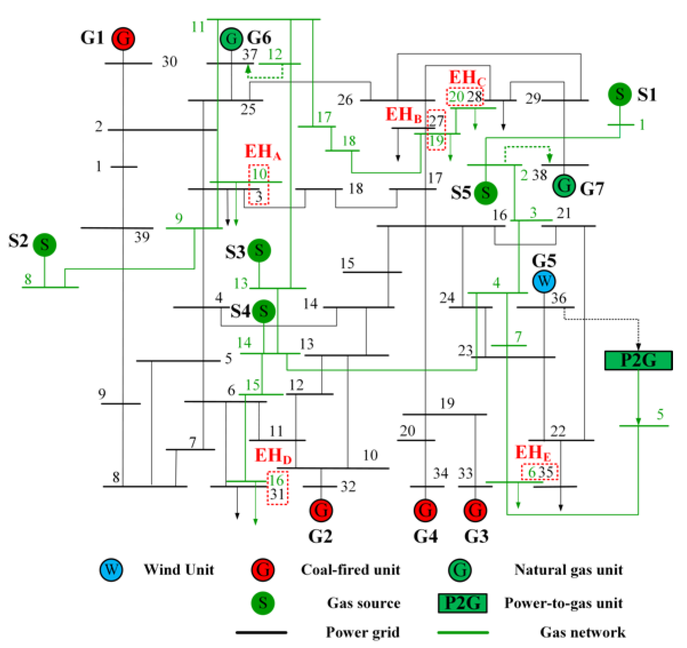
4.1. A. Modified IEEE 39-Bus Power System/Belgian 20-Node Natural Gas System

4.1.1. Basic Data of the System

The modified electric-gas IES is shown in Figure 4. The power system includes four coal-fired units G1–G4, a wind turbine unit G5, and two gas-fired units G6–G7. The parameters of the thermal power units are listed in

Table 1. Parameters of the thermal power units.

Unit	Type	Capacity /(MW)	Cost Coefficient /($/MW)	Emission Intensity /(t CO2/MW)
G1	Coal-fired	1040	35	1.280
G2	Coal-fired	725	35	1.300
G3	Coal-fired	652	35	1.290
G4	Coal-fired	508	35	1.270
G6	Gas-fired	564	\	0.564
G7	Gas-fired	865	\	0.550

[33,34]. Typical forecast data of wind turbine output were directly employed, as in other studies [27,35]. Wind turbine G5 had a cost coefficient of 15 $/MW and carbon emission intensity of 0.006 t CO₂/MW. The natural gas system contained five gas sources, whose parameters are listed in

Table 2. Parameters of the natural gas sources.

Capacity /(MBtu/h)	Cost Coefficient /($/MBtu)	Emission Intensity /(t CO2/MBtu)	Capacity /(MBtu/h)	Cost Coefficient /($/MBtu)
S1	15,000	11.6	0.0566	1.300
S2	20,000	10.8	0.0566	1.290
S3	1000	12.0	0.0566	1.270
S4	250	10.2	0.0566	0.564
S5	250	10.0	0.0566	0.550

[32]. The power grid and gas network were coupled by the P2G equipment with a capacity of 50 MW. Five power/gas loads were paired to form five energy hubs: $\mathit{E}{\mathit{H}}_{\mathit{A}}–\mathit{E}{\mathit{H}}_{\mathit{E}}$. The detailed data of the power load and gas load of each EH are listed in

Table 3. Data of the energy hubs.

EH	Power Load/(MW)	Gas Load/(MBtu/h)
EHA	913.6	526.2
EHB	685.2	25.0
EHC	685.2	158.6
EHD	456.8	1290.9
EHE	456.8	333.5

. The per-unit values of the 24 h maximum wind power outputs, power demands, and gas demands are shown in Figure 5. The base values of the wind power output, power load, and gas load were 658.8 MW, 3197.6 MW, and 2334.2 MBtu/h, respectively. The relevant data of the ladder-type carbon prices are shown in

Table 4. Parameters of the ladder-type carbon price.

Piecewise Interval	Carbon Price/($/t CO2)
$0~X_{i,minavg}$	${\lambda }_1=-5$
$X_{i,minavg}~X_{i,midavg}$	${\lambda }_2=15$
$X_{i,midavg}~X_{i,maxavg}$	${\lambda }_3=30$
$X_{i,maxavg}~\infty$	${\lambda }_4=60$
$0~X_{i,minavg}$	${\lambda }_1=-5$

.

4.1.2. Formation of the Ladder-Type Carbon Trading Mechanism for the Five EHs

It can be observed from Figure 4 that there are five EHs, denoted as A–E for convenience. Thus, the entire alliance is $N=\left\{A, B, C, D, E\right\}$, and there are 31 non-empty sub-alliances of $N$. Taking $t=1$ as an example, the economic dispatch model of the IES is solved under the conditions of different sub-alliances, and the results for the system carbon emission responsibilities are shown in

Table 5. The carbon emission responsibility of each sub-alliance.

Sub-Alliance	Carbon Emission Responsibility /(t CO2)	Sub-Alliance	Carbon Emission Responsibility /(t CO2)
{A}	574.70	\	\
{B}	375.29	{A, B}	1075.64
{C}	382.63	{A, C}	1087.93
{D}	48.77	{A, D}	1124.59
{E}	10.40	{A, E}	1089.93
{B, C}	1067.71	{A, B, C}	1480.67
{B, D}	929.60	{A, B, D}	1505.31
{B, E}	883.47	{A, B, E}	1476.86
{C, D}	939.98	{A, C, D}	1526.90
{C, E}	897.98	{A, C, E}	1489.16
{D, E}	574.60	{A, D, E}	1139.50
{B, C, D}	1120.59	{A, B, C, D}	1550.08
{B, C, E}	1082.62	{A, B, C, E}	1508.31
{B, D, E}	1120.91	{A, B, D, E}	1520.23
{C, D, E}	1130.49	{A, C, D, E}	1541.82
{B, C, D, E}	1520.13	{A, B, C, D, E}	2458.65

.

Taking $E{H}_A$ as an example, it can be obtained from Equations (20)–(23):

$$X_{A,max}=max\left\{C\left(S\cup \left\{A\right\}\right)-C\left(S\right)\right\}=C\left(A,B, D,E\right)-C\left(B,D,E\right)=399.32 tC{O}_2$$

(55)

$$X_{A,min}=min\left\{C\left(S\cup \left\{A\right\}\right)-C\left(S\right)\right\}=C\left(A,D\right)-C\left(D\right)=1075.82 tC{O}_2$$

(56)

$$X_{A,mid}={\displaystyle \sum }_S\frac{\left|S\right|!\left(5-\left|S\right|-1\right)!}{5!}\left[C\left(S\cap \left\{A\right\}\right)-C\left(S\right)\right]=674.8 tC{O}_2$$

(57)

where $S$ is any sub-alliance containing $A$, and $\left|S\right|$ is the number of members in the sub-alliance $S$.

In analogy with Equations (55)–(57), the carbon emission responsibility boundaries for the other 23 h can be obtained. Thus, the average value of the 24-h $E{H}_A$ carbon responsibility boundaries is

$$X_{A,minavg}=694.80 tC{O}_2$$

(58)

$$X_{A,midavg}=904.32 tC{O}_2$$

(59)

$$X_{A,maxavg}=1105.66 tC{O}_2$$

(60)

In summary, the ladder-type carbon trading cost of $E{H}_A$ at time $t$ is:

$$C_{A,t}^{CT}=\{\begin{array}{lr}{\lambda }_1(694.80-E_{A,t})& 0\le E_{A,t}<694.80\\ {\lambda }_2(E_{A,t}-694.80)& 694.80\le E_{A,t}<904.32\\ 209.52{\lambda }_2+{\lambda }_3(E_{A,t}-904.32)& 904.32\le E_{A,t}<1105.66\\ 209.52{\lambda }_2+201.34{\lambda }_3+{\lambda }_4(E_{A,t}-1105.66)& E_{A,t}\ge 1105.66\end{array}$$

(61)

On this basis, the 24-h carbon emission responsibility grades of the five EHs can be divided after the allocation of the carbon responsibility of the load side based on the Shapley value method. The results are shown in Figure 6. The carbon responsibility grades from low to high are represented in green, yellow, orange, and red, respectively. The three dashed horizontal lines represent the 24 h averages of the responsibility boundaries for different color grades. Based on these three averages, a one-day ladder-type carbon price can be formed for each EH, which will be used to calculate the carbon trading cost later.

The calculation results of the carbon emission responsibility boundaries are closely related to the load value and location. In particular, the Shapley value $X_{mid}$ (i.e., the upper boundary of the yellow grade) depends largely on the load value. Due to the low-carbon intensity of natural gas, the carbon emissions of each EH are mainly determined by the power load value. The power loads of $E{H}_B$ and $E{H}_C$ are equal, so it can be seen from Figure 6 that their carbon emission responsibility grades were basically similar, as were $E{H}_D$ and $E{H}_E$. Due to the large power load of $E{H}_A$, its carbon emission responsibility boundaries were also obviously higher than those of the other four EHs. However, the carbon emission responsibility boundaries of $E{H}_E$ were slightly lower than those of $E{H}_D$. This is because the location of $E{H}_E$ was closer to the wind turbine, and a higher proportion of the power consumed came from wind power. From the above analysis, it can be seen that the Shapley value method can reasonably and effectively determine the carbon emission responsibility grades among the EHs.

4.2. Analysis of Scenarios with and without Wind Power

4.2.1. Scenario 1: Without Wind Power

In order to better study the impact of the two-stage model on the IES, the wind turbine G5 on bus 36 in the power system was replaced by a 300 MW coal-fired unit with a carbon emission intensity of 1.28 t CO₂/MWh as the blank control group. Based on the Shapley value method, the 24 h carbon emission responsibility boundaries of the five EHs in the IES were calculated again, and the 24-h average values were used to divide the ladder-type carbon price grades, as shown in Figure 7. Comparing Figure 6 and Figure 7, it can be seen that the 24 h trend of the Shapley value $X_{mid}$ (i.e., the upper boundary of the yellow grade) for the same EH in the two different scenarios was basically consistent and similar to the load curve, since the load values did not change. However, in Scenario 1, the profitable grades were significantly higher than those in the scenario with wind power, especially at night. This is because the carbon intensity of wind power was much lower than those of thermal power and natural gas. In Scenario 1, the EH consumes energy with a high carbon intensity, causing it to emit more carbon with the same load. Therefore, in the calculation of the Shapley value method, it is reasonable that the minimum carbon emission responsibility boundary (i.e., the upper boundary of the green grade) can be adjusted according to the actual carbon emissions of the EH.

After applying the two-stage model considering the DR, the total power/gas demand, energy supply cost, carbon trading cost, and the carbon emissions before and after the optimization are shown in Figure 8 and Figure 9, respectively. As shown in Figure 8, in an IES without wind power, the model could effectively shave the peaks and fill valleys for the system load. Figure 9 shows that the energy supply cost and carbon emissions remained basically unchanged before and after the optimization because there was no low-carbon and low-cost energy injection. However, the carbon trading cost was visibly reduced by approximately 28.9%. This is because, after peak shaving and valley filling under the condition of the constant total load, when optimizing the carbon trading cost, the daytime load could jump from the relatively high-price carbon responsibility grade toward the lower price grade, and the night load increased as much as possible within the original price grade to achieve the lowest total carbon trading cost. From the above results, it can be seen that the model proposed in this paper can effectively guide the load to shave peaks and fill valleys, thus reducing the carbon trading cost.

4.2.2. Scenario 2: With Wind Power

In Scenario 2, the IES structure diagram and carbon emission responsibility grades are shown in Figure 4 and Figure 6, respectively. Figure 10 shows that the two-stage model can still effectively promote load shaving and valley filling in Scenario 2. In Figure 11, the wind power consumption was greatly improved after the response at 1–8 h and 22–24 h. Wind power has the characteristics of low carbon and low cost. Under the action of the two-stage model, the system load can respond in the direction of consuming as much wind power as possible. Before the optimization, except for 8–22 h, there was abandoned wind power for the rest of the time, and the wind power consumption rate throughout the day was only 43.2%. After the optimization, the night load actively participated in the response to consume excess wind power. Consequently, the wind-power consumption rate reached 93.0%.

Figure 12 presents the energy supply cost, carbon trading cost, and carbon emissions before and after the optimization in Scenario 2. Compared with Figure 9, Figure 12 shows that the system energy supply cost and carbon emissions were significantly reduced after the optimization in the scenario including low-carbon and low-cost wind power. Specifically, the energy supply cost, carbon trading cost, and total carbon emissions were reduced by 2.9%, 21.7%, and 6.2%, respectively. From the above results of Scenario 2, it can be proven that the proposed model can not only effectively promote the load peak shaving and valley filling and reduce the load-side carbon trading cost, but also greatly improve the renewable energy consumption capacity of the IES, reducing the carbon emissions and energy supply cost.

4.2.3. Scenario 3: With Different Wind Penetration Rates

To investigate the effect of the two-stage model on the IES with different renewable energy penetration rates, the carbon emissions and percentages of carbon emission reduction after the optimization were studied with the wind power penetration rate (installed wind power capacity/system maximum system load) increasing from 20% to 80% in steps of 10%. As shown in Figure 13, an increase in the penetration rate led to the gradual reduction in the system carbon emissions, and the percentage of carbon reduction after the optimization remained basically stable, with a slight increase from 6.2% to 6.8%. Therefore, with the growth in renewable energy, the two-stage model considering the DR proposed in this paper can still effectively reduce carbon emissions.

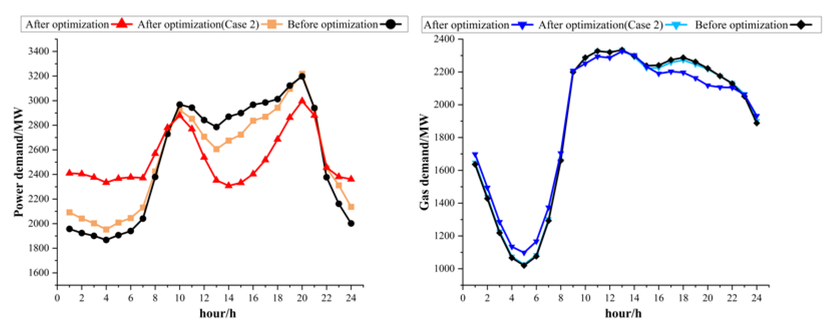
4.3. Discussion of the DR Mechanism

From the above scenario analysis considering the load-side carbon trading cost as the objective function, the system could achieve the load peak shaving and valley filling through the DR, thereby reducing the system carbon emission cost. To further explore the essential mechanism of the DR, the following discussion focused on two factors: carbon emissions and ladder-type carbon prices, which determine the objective function of the second stage.

4.3.1. Influence Mechanism of the Ladder-Type Carbon Prices on the DR

The influence mechanism of the ladder-type carbon price on the DR is shown in Figure 14. The direction of the DR is determined by the carbon price of the current load carbon emission responsibility grade. More specifically, the daytime load at a relatively high-price grade shifts the carbon emission responsibility toward a lower-price grade through a negative response. The night load at a low-price grade responds positively within the original carbon price grade as much as possible to maintain the total load conserved throughout the day. Thus, the carbon price gap can guide the DR to reduce the carbon trading cost on the load side.

To demonstrate the promoting effect of the carbon price gap on the DR, two different carbon pricing cases were compared in Scenario 2.

• Case 1: Constant carbon pricing;
• Case 2: Ladder-type carbon pricing.

Case 2 adopted the ladder-type carbon price model proposed in this paper and its parameters are shown in Table 4. As the blank control group, Case 1 adopted a constant carbon price of 7.5 $/t CO₂. Thus, Case 1 and Case 2 were equal in the carbon trading cost before the two-stage optimization. The results before and after the optimization of the two cases are shown in Figure 15 and Figure 16. In Figure 15, the demand response after the optimization in Case 2 was more obvious than that in Case 1. In Figure 16, after the optimization, the carbon trading cost and carbon emissions in Case 2 were lower than those in Case 1. The carbon trading cost reduction percentages of Case 1 and Case 2 were 1.0% and 21.7%, respectively. The carbon emission reduction percentages of Case 1 and Case 2 were 1.9% and 6.2%, respectively. These results confirm that the carbon price gap can better guide the DR to reduce carbon emissions and the carbon trading cost.

4.3.2. Influence Mechanism of Carbon Emissions on the DR

The load carbon emissions depend on the load carbon intensity and load value. Therefore, the impact of carbon emissions on the DR can be further investigated by focusing on the carbon intensity. The following discussion takes the power demand response in Scenario 2 as an example. According to the principle of proportional sharing [29], the carbon intensity of each bus is determined by the power component injected into the bus, and its value is the weighted average of the carbon intensity of each power component. The power composition of the five power loads in Scenario 2 is shown in Figure 17. The corresponding results of the bus carbon intensities are indicated by the blue line in Figure 18.

Figure 18 shows the relationship between the response value of each power load and bus carbon intensity. It can be seen from Figure 18 that in the period when the carbon intensity was relatively high, the load reduced the consumption of high-carbon power through a negative response. During the period when the carbon intensity was relatively low, the load increased the consumption of low-carbon power through a positive response to meet the conservation of total power demand. The response value is affected by the relative size of the carbon intensity, response range, response change ability, etc. Therefore, the carbon trading cost on the load side can be reduced by directly reducing the carbon emissions from energy consumption. Therefore, the carbon intensity difference caused by the renewable energy connected to the system can promote the DR to reduce the carbon trading cost on the load side.

4.4. Discussion of Three Carbon Reduction Methods

To study whether the proposed method had a superior carbon reduction in the IES, three carbon reduction methods in the existing related research and this paper were compared As shown in

Table 6. Details of the three carbon reduction methods in the existing related research and this paper.

Method	Carbon Trading		DR	Reference
	Source-Side	Load-Side
Method 1	✔			[9]
Method 2			✔	[19]
Method 3		✔	✔	This paper

, Method 1, referenced from [9], is the low-carbon economic dispatch considering the source-side carbon trading. Method 2, referenced from [19], is the economic dispatch considering the DR driven by the time-of-use tariff. Method 3, which was proposed in this paper, is the economic dispatch considering the DR driven by the load-side carbon trading.

The three methods were tested in the modified IEEE 39-bus power system/Belgian 20-node natural gas system of this paper, and the total carbon emissions and wind power consumption rates of the system before and after adopting the three methods were obtained, as shown in Figure 19. The carbon reduction effect of the proposed Method 3 was 281.8% and 203.7% of Method 1 and Method 2, respectively. The wind power consumption rate of the proposed Method 3 was 178.3% and 135.3% of Method 1 and Method 2, respectively. Therefore, the proposed method had significant superiority in promoting the wind power consumption and reducing the system carbon emissions compared with Methods 1 and 2.

5. Conclusions

In this paper, a two-stage low-carbon economic dispatch model of an electric-gas integrated energy system considering the demand response was proposed. In the first stage, the economic dispatch of the integrated energy system was carried out with the objective of minimizing the energy supply cost, and the carbon emission responsibility of the load side was obtained based on the carbon emission flow theory. In the second stage, the low-carbon demand response optimization was carried out with the objective of minimizing the carbon trading cost on the load side. Additionally, a reward and punishment ladder-type carbon trading mechanism, which was used to calculate the carbon trading cost in the second stage, was formulated for each energy hub based on the Shapley value method. Cases based on a modified IEEE 39-bus power system/Belgian 20-node natural gas system were studied to demonstrate the effectiveness of the proposed model. By analyzing the all-thermal-power scenario, wind-included scenario, and scenario with varying wind power penetration rates, four conclusions can be drawn.

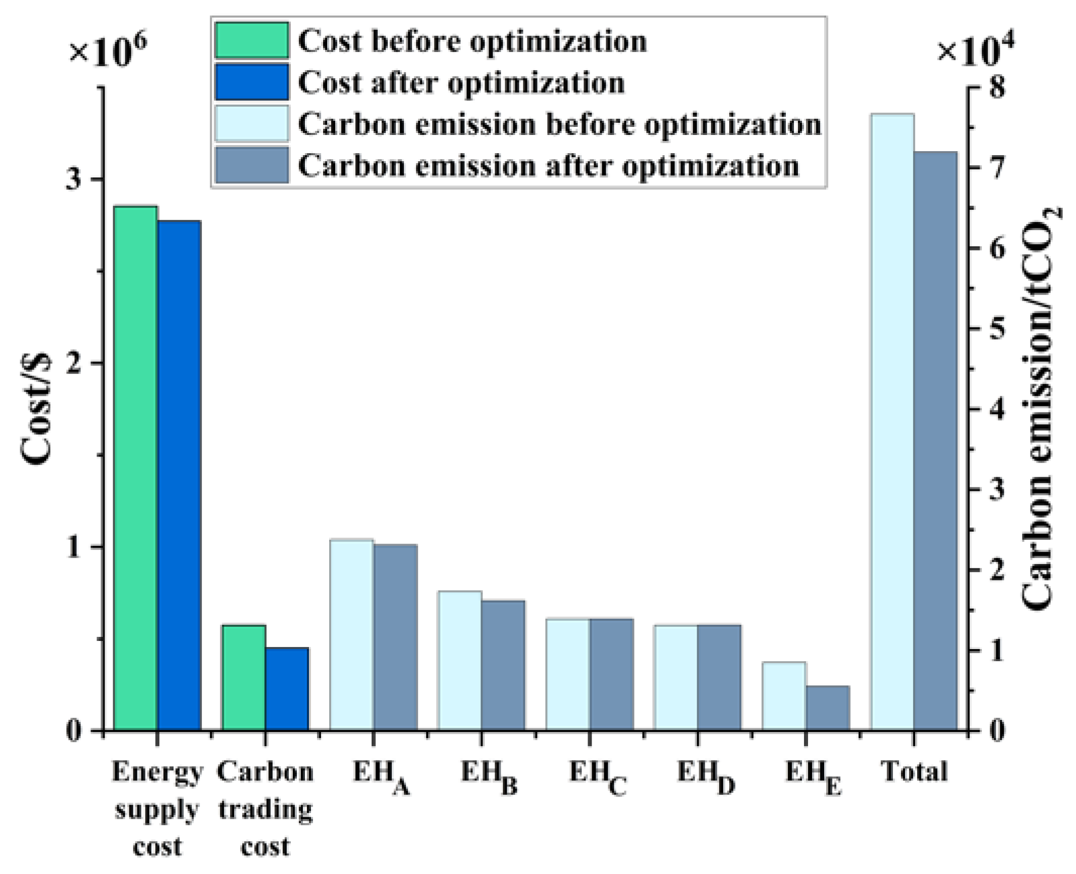
• The two-stage model proposed in this paper could effectively reduce the peak-to-valley difference, enhance the ability of the system to consume wind power, and reduce the system carbon emissions by 6.2% and the carbon trading cost by 21.7%.
• As the wind power penetration rate of the system increased from 20% to 80%, the carbon reduction effect of the model remained basically stable, with a slight increase from 6.2% to 6.8%. Therefore, with the growth in renewable energy, the two-stage model considering the demand response proposed in this paper can still effectively reduce carbon emissions.
• Based on the Shapley value method, the user-side ladder-type carbon trading mechanism was thus formulated. The method proposed in this paper drives the demand response through user-side carbon trading. By comparing the proposed method with the other two related existing methods, the carbon emission reduction effect of the proposed method was 281.8% and 203.7% of the other two methods, respectively. Therefore, the proposed method was proven to have superiority over the other two methods in carbon reduction.

However, there were some limitations in this paper. For example, in the demand response, the loads can be further classified into important loads, shiftable loads, and adjustable loads. Furthermore, the impact of the load-side energy storage and distributed renewable energy was not considered. Based on this study, future research on the low-carbon demand response can be conducted by considering factors such as load-side energy storage, distributed renewable energy, and load types.

References

1. Moore, F.C.; Lacasse, K.; Mach, K.J.; Shin, Y.A.; Gross, L.J.; Beckage, B. Determinants of emissions pathways in the coupled climate–social system. Nature 2022, 603, 103–111. [Google Scholar] [CrossRef] [PubMed]
2. Sognnaes, I.; Gambhir, A.; van de Ven, D.-J.; Nikas, A.; Anger-Kraavi, A.; Bui, H.; Campagnolo, L.; Delpiazzo, E.; Doukas, H.; Giarola, S.; et al. A multi-model analysis of long-term emissions and warming implications of current mitigation efforts. Nat. Clim. Change 2021, 11, 1055–1062. [Google Scholar] [CrossRef]
3. Huang, W.; Zhang, N.; Cheng, Y.; Yang, J.; Wang, Y.; Kang, C. Multienergy Networks Analytics: Standardized Modeling, Optimization, and Low Carbon Analysis. Proc. IEEE 2020, 108, 1411–1436. [Google Scholar] [CrossRef]
4. Wang, Y.; Wang, Y.; Huang, Y.; Yu, H.; Du, R.; Zhang, F.; Zhang, F.; Zhu, J. Optimal Scheduling of the Regional Integrated Energy System Considering Economy and Environment. IEEE Trans. Sustain. Energy 2019, 10, 1939–1949. [Google Scholar] [CrossRef]
5. Liu, N.; Wang, J.; Wang, L. Hybrid Energy Sharing for Multiple Microgrids in an Integrated Heat–Electricity Energy System. IEEE Trans. Sustain. Energy 2019, 10, 1139–1151. [Google Scholar] [CrossRef]
6. Zhu, X.; Yang, J.; Liu, Y.; Liu, C.; Miao, B.; Chen, L. Optimal Scheduling Method for a Regional Integrated Energy System Considering Joint Virtual Energy Storage. IEEE Access 2019, 7, 138260–138272. [Google Scholar] [CrossRef]
7. Zhang, Z.; Jing, R.; Lin, J.; Wang, X.; van Dam, K.H.; Wang, M.; Meng, C.; Xie, S.; Zhao, Y. Combining agent-based residential demand modeling with design optimization for integrated energy systems planning and operation. Appl. Energy 2020, 263, 114623. [Google Scholar] [CrossRef]
8. Fu, Y.; Sun, Q.; Wennersten, R. The effect of correlation of uncertainties on collaborative optimization of integrated energy system. Energy Rep. 2021, 7, 586–592. [Google Scholar] [CrossRef]
9. Wang, R.; Wen, X.; Wang, X.; Fu, Y.; Zhang, Y. Low carbon optimal operation of integrated energy system based on carbon capture technology, LCA carbon emissions and ladder-type carbon trading. Appl. Energy 2022, 311, 118664. [Google Scholar] [CrossRef]
10. Chen, L.; Msigwa, G.; Yang, M.; Osman, A.I.; Fawzy, S.; Rooney, D.W.; Yap, P.S. Strategies to achieve a carbon neutral society: A review. Environ. Chem. Lett. 2022, 1–34. [Google Scholar] [CrossRef]
11. Huang, Y.; Ding, T.; Li, Y.; Li, L.; Chi, F.; Wang, K.; Wang, X.; Wang, X. Decarbonization Technologies and Inspirations for the Development of Novel Power Systems in the Context of Carbon Neutrality. Proc. CSEE 2021, 41, 28–51. [Google Scholar] [CrossRef]
12. Peñasco, C.; Anadón, L.D.; Verdolini, E. Systematic review of the outcomes and trade-offs of ten types of decarbonization policy instruments. Nat. Clim. Change 2021, 11, 257–265. [Google Scholar] [CrossRef]
13. Miao, B.; Lin, J.; Li, H.; Liu, C.; Li, B.; Zhu, X.; Yang, J. Day-Ahead Energy Trading Strategy of Regional Integrated Energy System Considering Energy Cascade Utilization. IEEE Access 2020, 8, 138021–138035. [Google Scholar] [CrossRef]
14. Peng, Q.; Wang, X.; Kuang, Y.; Wang, Y.; Zhao, H.; Wang, Z.; Lyu, J. Hybrid energy sharing mechanism for integrated energy systems based on the Stackelberg game. CSEE J. Power Energy Syst. 2021, 7, 911–921. [Google Scholar] [CrossRef]
15. Xu, D.; Zhou, B.; Wu, Q.; Chung, C.Y.; Li, C.; Huang, S.; Chen, S. Integrated Modelling and Enhanced Utilization of Power-to-Ammonia for High Renewable Penetrated Multi-Energy Systems. IEEE Trans. Power Syst. 2020, 35, 4769–4780. [Google Scholar] [CrossRef]
16. Gu, N.; Wang, H.; Zhang, J.; Wu, C. Bridging Chance-Constrained and Robust Optimization in an Emission-Aware Economic Dispatch With Energy Storage. IEEE Trans. Power Syst. 2022, 37, 1078–1090. [Google Scholar] [CrossRef]
17. Wang, Y.; Wang, Y.; Huang, Y.; Yang, J.; Ma, Y.; Yu, H.; Zeng, M.; Zhang, F.; Zhang, Y. Operation optimization of regional integrated energy system based on the modeling of electricity-thermal-natural gas network. Appl. Energy 2019, 251, 113410. [Google Scholar] [CrossRef]
18. Misconel, S.; Zöphel, C.; Möst, D. Assessing the value of demand response in a decarbonized energy system—A large-scale model application. Appl. Energy 2021, 299, 117326. [Google Scholar] [CrossRef]
19. Lv, G.; Cao, B.; Dexiang, J.; Wang, N.; Li, J.; Chen, G. Optimal scheduling of regional integrated energy system considering integrated demand response. CSEE J. Power Energy Syst. 2021, 1–10. [Google Scholar] [CrossRef]
20. Yu, B.; Sun, F.; Chen, C.; Fu, G.; Hu, L. Power demand response in the context of smart home application. Energy 2022, 240, 122774. [Google Scholar] [CrossRef]
21. Guo, B.; Weeks, M. Dynamic tariffs, demand response, and regulation in retail electricity markets. Energy Econ. 2022, 106, 105774. [Google Scholar] [CrossRef]
22. Yuan, G.; Gao, Y.; Ye, B.; Liu, Z. A bilevel programming approach for real-time pricing strategy of smart grid considering multi-microgrids connection. Int. J. Energy Res. 2021, 45, 10572–10589. [Google Scholar] [CrossRef]
23. Yuan, G.; Gao, Y.; Ye, B. Optimal dispatching strategy and real-time pricing for multi-regional integrated energy systems based on demand response. Renew. Energy 2021, 179, 1424–1446. [Google Scholar] [CrossRef]
24. Zhou, T.; Kang, C.; Xu, Q.; Chen, Q. Preliminary Theoretical Investigation on Power System Carbon Emission Flow. Autom. Electr. Power Syst. 2012, 36, 38–43. [Google Scholar]
25. Kang, C.; Zhou, T.; Chen, Q.; Wang, J.; Sun, Y.; Xia, Q.; Yan, H. Carbon Emission Flow From Generation to Demand: A Network-Based Model. IEEE Trans. Smart Grid 2015, 6, 2386–2394. [Google Scholar] [CrossRef]
26. Cheng, Y.; Zhang, N.; Wang, Y.; Yang, J.; Kang, C.; Xia, Q. Modeling Carbon Emission Flow in Multiple Energy Systems. IEEE Trans. Smart Grid 2019, 10, 3562–3574. [Google Scholar] [CrossRef]
27. Cheng, Y.; Zhang, N.; Zhang, B.; Kang, C.; Xi, W.; Feng, M. Low-Carbon Operation of Multiple Energy Systems Based on Energy-Carbon Integrated Prices. IEEE Trans. Smart Grid 2020, 11, 1307–1318. [Google Scholar] [CrossRef]
28. Electric power transmission and distribution losses. OECD/IEA 2018.
29. Bialek, J. Tracing the Flow of Electricity. IEE Proc. Gener. Transm. Distrib. 1996, 143, 313–320. [Google Scholar] [CrossRef] [Green Version]
30. Zhou, Q.; Feng, D.; Xu, C.; Feng, C.; Sun, T.; Ding, T. Methods for Allocating Carbon Obligation in Demand Side:a Comparative Study. Autom. Electr. Power Syst. 2015, 7, 153–159. [Google Scholar]
31. Yang, L.; Xu, Y.; Sun, H.; Zhao, X. Two-Stage Convexification-Based Optimal Electricity-Gas Flow. IEEE Trans. Smart Grid 2020, 11, 1465–1475. [Google Scholar] [CrossRef]
32. De Wolf, D.; Smeers, Y. The Gas Transmission Problem Solved by an Extension of the Simplex Algorithm. Manag. Sci. 2000, 46, 1454–1465. [Google Scholar] [CrossRef] [Green Version]
33. Zimmerman, R.D.; Murillo-Sánchez, C.E. MATPOWER User’s Manual; Power Systems Engineering Research Center: Washington, DC, USA, 2011. [Google Scholar]
34. Wang, Y.; Zhou, S.; Wang, Y.; Qin, X.; Chen, F.; Ou, X. Comprehensive assessment of the environmental impact of China’s nuclear and other power generation technologies. J. Tsinghua Univ. (Sci. Technol.) 2021, 61, 377–384. [Google Scholar] [CrossRef]
35. Cao, Y.; Wei, W.; Wu, L.; Mei, S.; Shahidehpour, M.; Li, Z. Decentralized Operation of Interdependent Power Distribution Network and District Heating Network: A Market-Driven Approach. IEEE Trans. Smart Grid 2019, 10, 5374–5385. [Google Scholar] [CrossRef]
Figure 1. The structure of an electric-gas IES.
Energies 15 03641 g001
Figure 2. The framework of the two-stage mathematical model.
Energies 15 03641 g002
Figure 3. The schematic diagram of the ladder-type carbon price.
Energies 15 03641 g003
Figure 4. The modified IEEE 39-bus power system and the Belgian 20-node gas system.
Energies 15 03641 g004
Figure 5. The modified IEEE 39-bus power system and the Belgian 20-node gas system.
Energies 15 03641 g005
Figure 6. The carbon emission responsibility grades of each EH allocated by the Shapley value method in the scenario with wind power.
Energies 15 03641 g006
Figure 7. The carbon emission responsibility grades of each EH allocated by the Shapley value in Scenario 1.
Energies 15 03641 g007
Figure 8. The total power/gas demand before and after the optimization in Scenario 1.
Energies 15 03641 g008
Figure 9. The energy supply cost, carbon trading cost, and carbon emissions of each EH before and after the optimization in Scenario 1.
Energies 15 03641 g009
Figure 10. The total power/gas demand before and after the optimization in Scenario 2.
Energies 15 03641 g010
Figure 11. The total power/gas demand before and after the optimization in Scenario 2.
Energies 15 03641 g011
Figure 12. The energy supply cost, carbon trading cost, and carbon emissions of each EH before and after the optimization in Scenario 2.
Energies 15 03641 g012
Figure 13. The carbon emissions and carbon reduction percentages before and after the optimization in different wind power penetration systems.
Energies 15 03641 g013
Figure 14. The influence mechanism of the ladder-type carbon price on the DR.
Energies 15 03641 g014
Figure 15. The power/gas demand before and after the optimization in Case 1 and Case 2.
Energies 15 03641 g015
Figure 16. The carbon trading cost and carbon emissions before and after the optimization in Case 1 and Case 2.
Energies 15 03641 g016
Figure 17. The power composition analysis diagram of each power load in Scenario 2.
Energies 15 03641 g017
Figure 18. The response analysis diagram of each power demand in Scenario 2.
Energies 15 03641 g018
Figure 19. The system carbon emissions and wind power consumption rates with the different methods.
Energies 15 03641 g019