Parameter Effect Analysis of Non-Darcy Flow and a Method for Choosing a Fluid Flow Equation in Fractured Karstic Carbonate Reservoirs

Abstract

Fractured karstic carbonate reservoirs have obvious multi-scale characteristics and severe heterogeneity due to the development of abundant karst caves and fractures with different scales. Darcy and non-Darcy flows coexist due to this property. Therefore, selecting the appropriate flow equations for different regions in the numerical simulation of fluid flows, particularly two-phase and multiphase flows, is a critical topic. This paper compares and analyses the displacement distance differences of waterfront travel using the Darcy, Forchheimer and Barree–Conway equations, as well as analyzes the influence of the Forchheimer constant, fluid viscosity, flow rate and absolute permeability on inertia action based on the Buckley–Leverett theory. The results show that the Forchheimer number/Reynolds number of water/oil two-phase flow is not a constant value and varies with water saturation, making it difficult to determine whether the inertial action should be considered solely based on these values; the influence of inertial action can be measured well by comparing the difference between the displacement distances of the waterflood front, and the quantitative standard is given for the selection of the flow equation of different regions by calculating the allowable error of the displacement distance of the waterflood front. The magnitude of the inertial effect is affected by the physical properties of the fluid and reservoir medium and the fluid velocity. The smaller the difference in the viscosity of the oil/water fluid, the smaller the inertial effect is. This technique was used a preliminary attempt to analyze the fractured karstic carbonate reservoirs at Tarim, and the results confirmed the validity of the method described in this article.

1. Introduction

Carbonate reservoirs are an important type of reservoir that contain 60% of the world’s total oil and gas reserves [1]; however, they differ from conventional reservoirs. Their storage space includes primary porosity, fractures, and karst caves; hence, their porosity scale ranges from millimeter to meter levels. Therefore, two types of flow regimes are present in fractured karst carbonate reservoirs: Darcy flow and non-Darcy flow. One group of researchers used reduced-order models and machine learning to forecast the production of flow by building a high-fidelity DFN model in an unconventional reservoir with fractures [2]. Furthermore, another study proposed the Darcy/non-Darcy coupled model for fluid flow where Darcy and non-Darcy flow coexist [3] (Yao, 2018). Thus, the choice of flow equations according to the fluid flow regimes is an essential part of reservoir simulations. At present, researchers depend mainly on qualitative analysis or the Reynolds number to distinguish the flowing regimes and flow equations. For example, non-Darcy flow usually occurs in near-wellbore regions, large-scale fractures, large karst caves and unconsolidated areas, and at Re = 10–1000. These expressions are qualitative or vague rather than quantitative. There is no specific definition or criteria for predicting non-Darcy flow in fractured karstic carbonate reservoirs; moreover, we do not know the accurate range of the near-wellbore region for non-Darcy flow at a given production rate, or under what conditions non-Darcy flow occurs for the given fractured karstic regions.

Researchers have set up several different fluid flow equations to describe Darcy and non-Darcy flows, including the Darcy, Forchheimer and Barree–Conway equations. The Darcy equations [4] (1856) are widely accepted to describe the behavior of linear fluids, while Forchheimer [5] (1901) proposed the Forchheimer equation to describe non-Darcy flow. Researchers [6,7,8,9,10] (Carman, 1974; Fand, 1987; Montillet, 2004) have found that the Forchheimer equation is unsuitable for high-velocity flow. Barree and Conway [11,12] (2004) proposed the Barree–Conway equation, which is a more general equation for non-linear flow. The Barree–Conway equation has a similar expression as the Darcy equation if the pressure gradient is expressed in terms of the apparent permeability. The Barree–Conway equation describes the entire range of flow velocities versus pressure gradient from Darcy to non-Darcy flow regimes. Since fluids change from Darcy flow to non-Darcy flow as the velocity increases, these flow regimes are located in different regions of the same reservoirs. Thus, how to distinguish these two types of flow regimes has become a significant issue.

Until now, two criteria have been widely used to identify the transition to non-Darcy flow from Darcy flow, namely the Reynolds number and the Forchheimer number. Chilton [13] (1931) obtained and refined the Reynolds number equation through fluid flow experiments with packed particles based on the turbulent flow equation according to the previous belief that non-Darcy flow was similar to turbulent flow. Owing to the difficulty of determining the particle diameter, Green [14] (1951) used the permeability (k) and non-Darcy coefficient (β) instead of the particle diameter. Ma [15] (1993) redefined the Reynolds number (Re) and gave a new criterion, the Forchheimer number (Fo). Not only are the definitions of the Reynolds number and the Forchheimer number inconsistent, but the critical values obtained in experiments are different for non-Darcy flow in porous media [15,16,17,18,19] recommended the Forchheimer number as a criterion for identifying non-Darcy flow due to its advantages of clear definition and wide applicability; the Forchheimer number is the ratio of the liquid–solid interaction pressure gradient to that of viscous resistance. The Reynolds number and Forchheimer number are both used to distinguish between Darcy flow and non-Darcy flow. However, there are still a few problems and obstacles. Furthermore, the critical values become more complex for multiphase flow.

It follows that the Darcy and non-Darcy flows are different flow regimes; however, they usually coexist when fluids flow in the same fractured karstic carbonate reservoir. For multiphase flow in the same fractured karstic reservoir, the non-Darcy equations are more complex than the Darcy equations. The Forchheimer coefficient in the Forchheimer equation is no longer a constant and instead varies with the parameters, which are related to the rock’s structure and the fluids’ properties, the denominator of the Barree–Conway equation becomes very complicated because the expression of apparent permeability is extremely complex. Thus, it not only requires considerable computation to implement the numerical simulation only using the Forchheimer or Barree–Conway equation for the whole reservoir, but also necessitates a greater effort to achieve stability in the numerical simulation. Therefore, the coupled model is a good choice [3] (Yao, 2018). Furthermore, most commercial software is developed based on the Darcy equations, and consequently there will be deviation in some cases with Darcy and non-Darcy flow coexistence. Thus, the following two problems arise: first, distinguishing Darcy flow and non-Darcy flow for choosing the flow equations, and second, evaluating and correcting the deviation in the numerical simulation using the Darcy equation to describe non-Darcy flow. Therefore, it is necessary to establish a method for evaluating the inertial effect and choosing the flow equations.

In this paper, the evolution of the non-Darcy flow mechanism and equations are reviewed. Then, analytical solutions are used to analyze the flow characteristics, compare the difference between Darcy flow and non-Darcy flow and analyze the effect of the parameters. Finally, a method is obtained for choosing the flow equations and estimating the displacement distance deviation of a waterflood front using the Darcy equation to describe non-Darcy flow.

2. Method of Comparing Darcy Flow and Non-Darcy Flows

2.1. Non-Darcy Flow Mechanism and Equations

Through physical experiments, researchers have found that after velocity increases to a certain value, the pressure gradient is no longer proportional to the flow velocity (Figure 1). The physical understanding of non-Darcy flow remains unclear, and there are two main opinions on it. One is that the non-Darcy effect is owing to turbulence, and the other is that inertial force causes the non-Darcy effect. Most researchers advocate for the second opinion, and an equation has been proposed to describe the additional pressure drop observed in non-Darcy flow at a high flow velocity. Bear [20] (1972) systematically gave three reasons to exclude turbulence as the cause for the non-Darcy effect. First, the linear term in the equation does not exist in turbulent flow; second, the transition from laminar to turbulent flow is rather sharp; and third, the critical Reynolds number (R_e) at which the transition starts is several orders of magnitude higher than that at which the non-Darcy effect begins. Moreover, it was concluded that the non-Darcy effect occurs because microscopic inertial effects alter the velocity and pressure fields.

The Forchheimer equation and Barree–Conway equation are the two main equations to describe non-Darcy flow. Although the equations are different from the Darcy equation in form, they have something in common. To some extent, the Forchheimer equation evolved from the Darcy equation according to the non-Darcy flow mechanism by adding an extra term; the Barree–Conway equation has a similar expression to the Darcy equation. The Forchheimer equation is widely accepted as follows:

$$-\nabla \varphi =\frac{\mu v}{k}+\beta \rho v\left|v\right|$$

(1a)

$$F_0=\frac{k\beta \rho v}{\mu }$$

(1b)

in which ϕ is the potential; μ is the viscosity; v is the superficial velocity; k is the absolute permeability; β is the Forchheimer coefficient; ρ is the fluid density; and F₀ is the Forchheimer number. On the right-hand side of the equation, the first term is the viscous term and the second term is the inertial term. When the viscous flow is at high rates, the second term becomes significant. The inertial term causes the differences in the flow behaviors and characteristics between Darcy flow and non-Darcy flow, and the value of β is substantial for the inertial effect. Usually, β is predicted using empirical formulas, and there are many different equations concerning the calculation of β. In this paper, we select one of them, which is based on an experimental study of single-phase flow.

$$\beta =\frac{C_{\beta }}{k^{5/4}{\varphi }^{3/4}}$$

(2)

The Forchheimer equation has a limited range of applicability for high-rate flow conditions; thus, the Barree–Conway equation [11,12] (Barree and Conway, 2004) was presented to describe the relationship between rate and potential gradient for the flow of the entire range of the Reynolds number:

$$-\nabla \varphi =\frac{\mu v}{k_{app}}$$

(3a)

$$k_{app}=k\left(k_{mr}+\frac{1-k_{mr}}{\left(1+R_e\right)}\right)$$

(3b)

$$k_{mr}=\frac{k_{min}}{k}$$

(3c)

$$R_e=\frac{\rho v}{\mu \tau }$$

(3d)

where k_app is apparent permeability; R_e is the Reynolds number; τ is the inverse of the characteristic length, which is related to the mean particle size of sand; k_min is the minimum permeability; and k_mr is the ratio of minimum permeability to Darcy permeability. Τ and k_mr are the key parameters in the equation, and τ is related to the permeability k and the mean size of the particles [11,12] (Barree, Conway, 2004). Usually, τ is a given value according to the particle size (Figure 2). The Reynolds number of Barree–Conway equation depends on the flow velocity and the inverse of the characteristic length τ. Theoretically, when k_mr is equal to 1, the Barree–Conway equation is reduced to the Darcy equation with constant permeability k; when k_mr is equal to zero, it converges to the Forchheimer equation. When the value of k_mr is set to zero, the Barree–Conway equation reduces to the form of the Forchheimer equation and we can obtain the relationship between these two equations and the relationship between τ and β for the single-phase.

$$\tau =\frac{1}{k\beta }$$

(4)

The main difference between the Forchheimer equation and the Barree-Conway equation is the different values of their parameters.

Darcy and non-Darcy flow are different but sometimes coexist underground, especially in complex fractured karstic carbonate media. The Forchheimer or Barree-Conway equations are used in the numerical simulation regardless of the magnitude of the non-Darcy effect, which will take large amounts of internal storage and calculating time. Similarly, the Darcy equation is not valid for high velocities because the inertial effect is ignored. The criteria for distinguishing the flow regimes of multiphase flow are more complex than those for single-phase flow. Establishing a method for evaluating the difference between them is necessary.

2.2. Analytical Solution of Darcy and Non-Darcy Equations

In an isothermal system, the mass-balance equations are as follows:

$$\frac{\partial }{\partial t}\left(\varphi S_{\alpha }{\rho }_{\alpha }\right)=-\nabla ·\left({\rho }_{\alpha }{v}_{\alpha }\right)+q_{\alpha };\alpha =w,o$$

(5)

where ϕ is the porosity of the medium, (−); S_α is the saturation of fluid α, (−); ρ_α is the density of fluid α (kg/m³); v_α is the volumetric flow rate of fluid α, (m/s); q_α is the mass source/sink term for fluid α (m³/s). The Forchheimer equation and the Barree–Conway equation can be extended for multiphase flow:

$$-\nabla P_{\alpha }=\frac{{\mu }_{\alpha }}{k{k}_{r\alpha }}{v}_{\alpha }+{\beta }_{\alpha }{\rho }_{\alpha }{v}_{\alpha }\left|v_{\alpha }\right|;\alpha =w,o$$

(6a)

$${\beta }_{\alpha }=\frac{C_{\beta }}{{\left(k{k}_{r\alpha }\right)}^{5/4}{\left[\varphi \left(S_{\alpha }-S_{\alpha r}\right)\right]}^{3/4}};\alpha =w,o$$

(6b)

$$-\nabla P_{\alpha }=\frac{{\mu }_{\alpha }{v}_{\alpha }}{k{k}_{r\alpha }\left[k_{mr}+\frac{\left(1-k_{mr}\right){\mu }_{\alpha }\tau }{{\mu }_{\alpha }\tau +{\rho }_{\alpha }\left|v_{\alpha }\right|}\right]};\alpha =w,o$$

(6c)

$$k_{mr}=\frac{k_{min}}{k}$$

(6d)

Two additional equations are required:

$${{\displaystyle \sum }}^{}{S}_{\alpha }=1,\alpha =w,o,$$

(7a)

$$P_w=P_o-P_c$$

(7b)

where P_c is the water-oil capillary pressure (Pa).

In an analytical solution of multiphase flow, the saturation profile can be obtained by using the method of characteristics [21,22] (Wu 1991; Wu 2001). The Buckley–Leverett flow conditions are assumed as follows: the multiphase fluids and porous media are incompressible; the capillary pressure gradient and gravity are ignored; the model is one-dimensional; and the fluid flows along the x-coordinate of a semi-infinite linear flow system. Based on these assumptions, acceptable approximations can be obtained. For one-dimensional flow, $v_{\alpha }$ can be expressed using the Forchheimer equation and Barree–Conway equation as follows:

$$\begin{gathered} v_{\alpha }=\frac{1}{2k{\beta }_{\alpha }{\rho }_{\alpha }}\left[-\frac{{\mu }_{\alpha }}{k_{r\alpha }}+\sqrt{{\left(\frac{{\mu }_{\alpha }}{k_{r\alpha }}\right)}^2-4k{\beta }_{\alpha }{\rho }_{\alpha }\frac{\partial P_{\alpha }}{\partial x}}\right];\alpha =w,o \\ {v}_{\alpha }=-\frac{1}{2{\mu }_{\alpha }{\rho }_{\alpha }}\left({\mu }_{\alpha }^2{S}_{\alpha }\tau +k_d{k}_{r\alpha }{k}_{mr}{\rho }_{\alpha }\frac{\partial P_{\alpha }}{\partial x}\right)+ \end{gathered}$$

(8a)

$$\frac{1}{2{\mu }_{\alpha }{\rho }_{\alpha }}\sqrt{{\left({\mu }_{\alpha }^2{S}_{\alpha }\tau +k_d{k}_{r\alpha }{k}_{mr}{\rho }_{\alpha }\frac{\partial P_{\alpha }}{\partial x}\right)}^2-4{\rho }_{\alpha }{k}_d{k}_{r\alpha }{k}_{mr}{\mu }_{\alpha }^2{S}_{\alpha }\tau \frac{\partial P_{\alpha }}{\partial x}};\alpha =w,o$$

(8b)

where $\frac{\partial P_{\alpha }}{\partial x}$ is along the x-coordinate. Then, the mass balance equation can be changed as follows:

$$-\frac{\partial v_{\alpha }}{\partial x}=\varphi \frac{\partial S_{\alpha }}{\partial t};\alpha =w,o$$

(9)

The fractional flow function for the wetting phase may be expressed in the following form:

$$f_w=\frac{v_w}{v_w+v_o}$$

(10)

$$f_o+f_w=1$$

(11)

Under the condition of the same pressure gradient, the inertial effect will affect the flow velocity of the fluid; hence, the displacement distances of waterflood fronts are different for the same volume of water injected. For the same fractured karstic media, the displacement distance calculated using the Darcy equation ignoring inertia is different from that using the non-Darcy equation; thus, there will be a displacement distance deviation of the waterflood front for non-Darcy flow when using the Darcy equation to simulate the fluid flow. In this paper, we introduce the distance deviation of the waterflood front to evaluate the difference between Darcy flow and non-Darcy flow:

$$Dev=\frac{L_D-L_{nD}}{L_D}\times 100\%$$

(12)

where $Dev$ is the distance deviation of the waterflood front (%); L_D is the distance of the waterflood front based on the Darcy equation (m); and L_nD is the distance of the waterflood front based on the non-Darcy equation (m).

Assuming that the physical flow model is a one-dimensional linear porous medium, and at first uniformly saturated with a nonwetting fluid (S_o = 0.8) and a wetting fluid (S_rw = 0.2), the volumetric injection rate is constant with the wetting fluid and imposed at the inlet (x = 0) starting from t = 0. The relative permeability can be estimated using the Brooks–Corey model [23] (Brooks and Corey, 1964). In this paper, all the fluids and formation parameters of the physical flow model are summarized in

Table 1. Parameters for physical flow model.

Parameters	Value	Unit
Porosity, ϕ	0.30
Absolute permeability, k	9.869 × 10−13	m2
Cross section area, A	1.0	m2
Length of model, L	5.0	m
Injection rate, qt	5.0 × 10−4	m3/s
Water viscosity, μw	1.0 × 10−3	Pa·s
Oil viscosity, μo	5.0 × 10−3	Pa·s
Residual water saturation, Swr	0.2
Residual oil saturation, Sor	0.2
Maximum relative permeability, krw,max	0.8
Maximum relative permeability, kro,max	0.8
Power index of relative permeability, nw	2
Power index of relative permeability, no	2
Density of water, ρw	1000	kg/m3
Density of oil, ρo	800	kg/m3
Forchheimer flow constant, Cβ	3.2 × 10−7	m3/2
Minimum permeability fraction, kmr	0.01
Inverse of characteristic length, τ	2.1× 103	m−1

.

Figure 3 shows the difference in the displacement distance of waterfront travel, water fractional flow, and flow velocities among the Darcy, Forchheimer, and Barree–Conway equations (τ = 2100, Figure 2) after the same injection volume of water. The solid lines represent the results of three equations and the dotted lines represent the results of modelling the Darcy and Forchheimer equations using the Barree–Conway equation by changing the values of k_mr and τ. In the water saturation profiles (Figure 3a), the result of the Barree–Conway equation is located between those of the Darcy and Forchheimer equations using the parameters in Table 1. The Barree–Conway equation will fit well with the result of the Darcy equation when k_mr is set to 1. However, when using the Barree–Conway equation to fit the result of the Forchheimer equation, k_mr is set to zero, and τ must be set to 700. In any case, the Barree–Conway equation fits the results of the Darcy and Forchheimer equations well in the water saturation profile. Comparing the flow velocities and the fractional flow (Figure 3b,c), when k_mr is set to 1, the results using the Barree–Conway equations coincide with those of the Darcy equation; however, the values using the Barree–Conway equation are inconsistent with those of Forchheimer equation when k_mr is set to zero and τ is set to 700. The reason for this difference is that the parameter values are different; τ is constantly dependent on the particle size and is equal to 700 in the Barree–Conway equation, but β_α varies with the parameters of the fluids and rock in the Forchheimer equation for two-phase flow. The variation of the Forchheimer/Reynolds number with the water saturation is shown in Figure 3d. Although changing the τ value of the Barree–Conway equation yields the same result in the water saturation profile as the Forchheimer equation, the Reynolds number differs from the Forchheimer number. The Reynolds numbers are the same when k_mr is equal to 0.01 and k_mr is equal to 0.0, because τ is equal to 2100.

In summary, non-Darcy flow is more complex than Darcy flow for multiphase flow, and the Forchheimer and Reynolds numbers are no longer constant and vary with the water saturation. The results of the three equations depend on the values of the parameters. Even if the water saturation of the Forchheimer equation and the Barree–Conway equation are the same, the values of flow velocity, Forchheimer number, and Reynolds number are different. The Forchheimer number has a definite physical meaning and represents the ratio of the viscous term to the inertial term. The water saturation profile of displacement can describe the deviation of non-Darcy flow from Darcy flow with respect to the distance of waterfront travel and water saturation.

3. Comparison of Darcy and Non-Darcy Equations Based on Analytical Solution

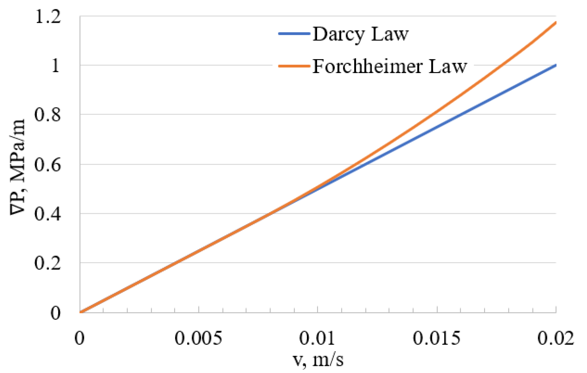
3.1. Comparison of Darcy and Forchheimer Equations

The inertial term in the Forchheimer equation contains the following parameters: flow velocity, Forchheimer constant C_β, porosity, absolute permeability, relative permeability and fluid saturation. The difference between the Forchheimer equation and the Darcy equation will now be compared and analyzed under the influence of the different parameters for two-phase flow. During the comparisons of the key parameters, the other parameters are given the values shown in Table 1.

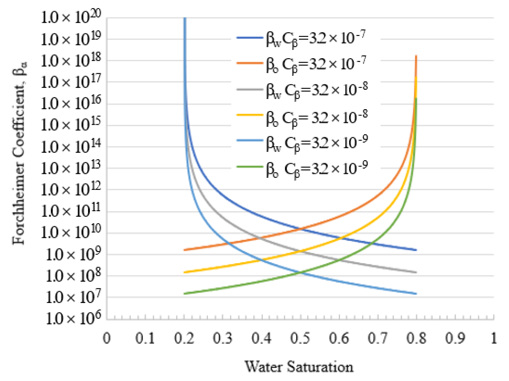
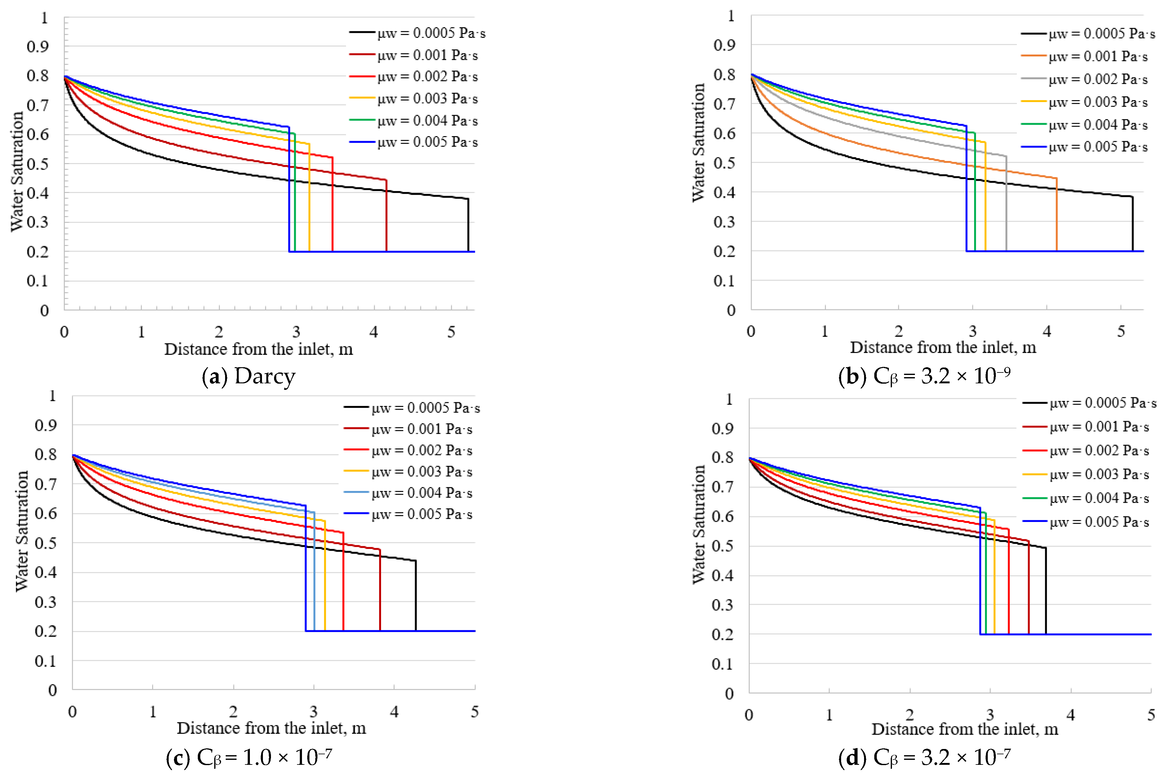
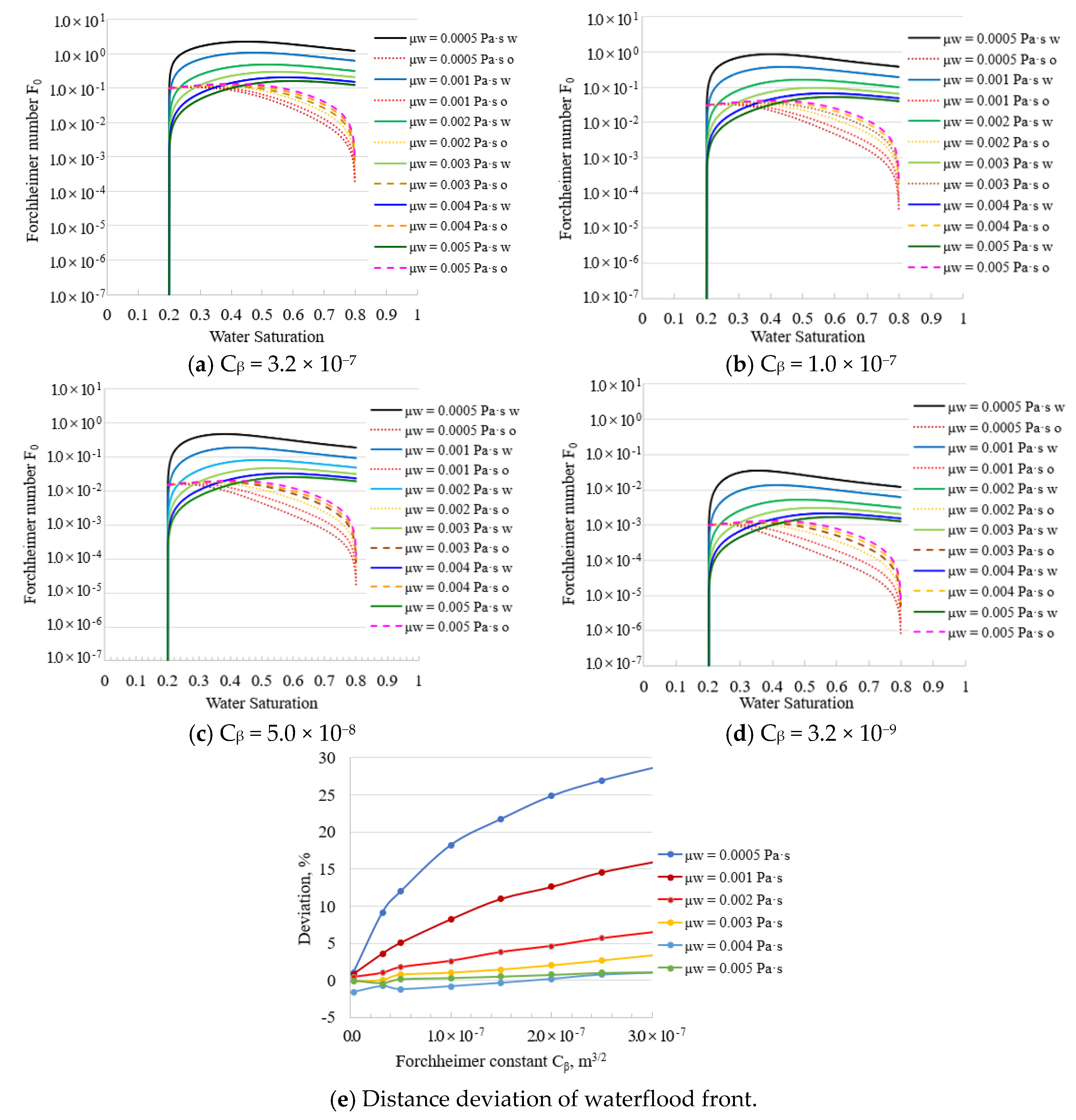
3.1.1. Forchheimer Constant C_β

Here, C_β is an important parameter for β_α and is related to the structure of the rock. Usually, the value of C_β is obtained through a physical experiment on rock cores. According to experimental tests, the value of C_β varies from 10⁻⁹ to 10⁻⁷ m^3/2. In this section, we will analyze the non-Darcy effect of rocks with a different structure using several different values of C_β from 3.2 × 10⁻⁹ to 3.2 × 10⁻⁷ m^3/2.

Figure 4 shows that the value of β_w changes with C_β and S_w for the same porous media. The β_w value changes from a very large value at the minimum water saturation to a minimum value at the maximum water saturation; conversely, the β_o value changes from a minimum value at low water saturation to a very large value at the maximum water saturation. Thus, the value of β_α is no longer constant and varies with the water saturation and C_β for multiphase fluids. The inertial force effect is largest when the oil begins to be displaced by the water and the inertial effect is especially substantial for very large or infinite at the beginning or end of the water saturation.

Figure 5 shows a comparison of the results of the Darcy equation and Forchheimer equation after the same volume of water is injected. The results of water saturation (Figure 5a) are different for the two-phase flow. The larger value of C_β displays a better sweeping efficiency and shorter front travel distance. When the value of C_β decreases, the line in the water saturation profile tends to be close to that of Darcy flow. When C_β is reduced to 3.2 × 10⁻⁹ m^3/2, the displacement saturation distributions of the Forchheimer equation are close to that of Darcy equation, which means the inertial force effect can be ignored. Figure 5b) displays the values of the Forchheimer number F₀ with the different water saturation and C_β values. Here, F₀ is also no longer constant and varies with the water saturation S_w and C_β. When C_β is equal to 3.2 × 10⁻⁷ m^3/2, the F₀ values of the water phase are larger than the others; the maximum is up to more than 1.00, and most values are between 0.10 and 1.10. The F₀ values of the oil phase are between 0.01 and 0.11, though they are smaller than those of the water phase. This means that the inertial force effect is obvious and cannot be ignored. When C_β equals 3.2 × 10⁻⁹ m^3/2, the F₀ values of the water phase are 0.013–0.006, and those of the oil phase are much smaller than 0.001. According to Zeng’s [24] (2006) results, the fluid flow belongs to Darcy flow, and the inertial force effect is negligible. The velocities of the fluids and the fractional flow curves all vary with the value of C_β (Figure 5e,d). When the value of C_β equals 3.2 × 10⁻⁹ m^3/2, the velocities and fractional flow curves nearly coincide with those of Darcy flow. The distance deviation of the waterflood front is also shown with a different Forchheimer constant C_β (Figure 5e). When the value of C_β is less than 5.0 × 10⁻⁸, the distance deviation of the waterflood front is less than 5.0%.

In summary, distinguishing between Darcy and non-Darcy flows and choosing the flow equation based on the value of the Forchheimer number is difficult, because the Forchheimer coefficient C_β and Forchheimer number F₀ of multiphase flows are not constant and vary with the water saturation. The β_w (or β_o) cannot be replaced by a constant value, because the values of β_w (or β_o) are very large or infinite at the beginning (or end) of the water saturation; however, the area scope is very small, and the inertial effect cannot be ignored. The displacement distance deviation of the waterflood front can quantify the difference between Darcy and non-Darcy flows well and help us evaluate the effect of non-Darcy flows in fractured karst reservoirs, choose the appropriate model and correct errors in the numerical simulation.

3.1.2. Fluid Viscosity

In this section, we will analyze the effect of fluid viscosity on the inertia, assuming that the constant viscosity of oil is 0.005 Pa·s and water viscosity takes the following values: 0.0005, 0.001, 0.002, 0.003, 0.004 and 0.005 Pa·s.

Figure 6 shows the water saturation profiles of the Darcy and Forchheimer flows with different ratios of fluid viscosity. When the viscosity difference between oil and water is the largest—namely, the water viscosity is 0.0005 Pa·s and oil viscosity is 0.005 Pa·s—the influence of the inertial effect is obvious in the displacement distance of waterfront travel and sweeping efficiency regardless of the values of C_β. As the water viscosity increases, the displacement distance of waterfront travel decreases. When the water viscosity is equal to that of the oil, the inertial effect tends to weaken because the displacement is similar to piston displacement. In general, the smaller the viscosity difference between the oil and water, the better the oil displacement efficiency.

For the same C_β value (Figure 7), the change in water viscosity affects the Forchheimer number. The water Forchheimer number decreases as the water viscosity increases, whereas the oil Forchheimer number increases. As C_β decreases from 3.2 × 10⁻⁷ to 3.2 × 10⁻⁹, the Forchheimer numbers of water and oil decrease as well. When C_β is equal to 3.2 × 10⁻⁷, most of the water Forchheimer numbers are greater than 0.1 and those of oil are greater than 0.01. The effect of inertial force cannot be ignored. According to the results in Figure 7e, the distance deviations of the waterflood front are less than 0.05 when the water viscosity is greater than or equal to 0.03. Therefore, the deviation is more credible for evaluating the effect of inertial force compared to the Forchheimer number. The distance deviations of the waterflood front with the different C_β and water viscosities are shown in Figure 7e. When the oil viscosity is equal to 0.005 Pa·s and the water viscosity is not greater than 0.003 Pa·s, the distance deviation of the waterflood front is not greater than 0.05, regardless of the value of C_β.

In summary, the inertial effect decreases as the oil–water viscosity ratio decreases. When the viscosities of the fluids are equal (i.e., the water viscosity increases from 0.0005 Pa·s to 0.005 Pa·s), the non-Darcy effect is minimal and can even be ignored. Determining whether to consider the inertial force only according to the value of the Forchheimer number is difficult, and the distance deviation of the waterflood front is more credible to evaluate the inertial effect and to correct the numerical simulation error.

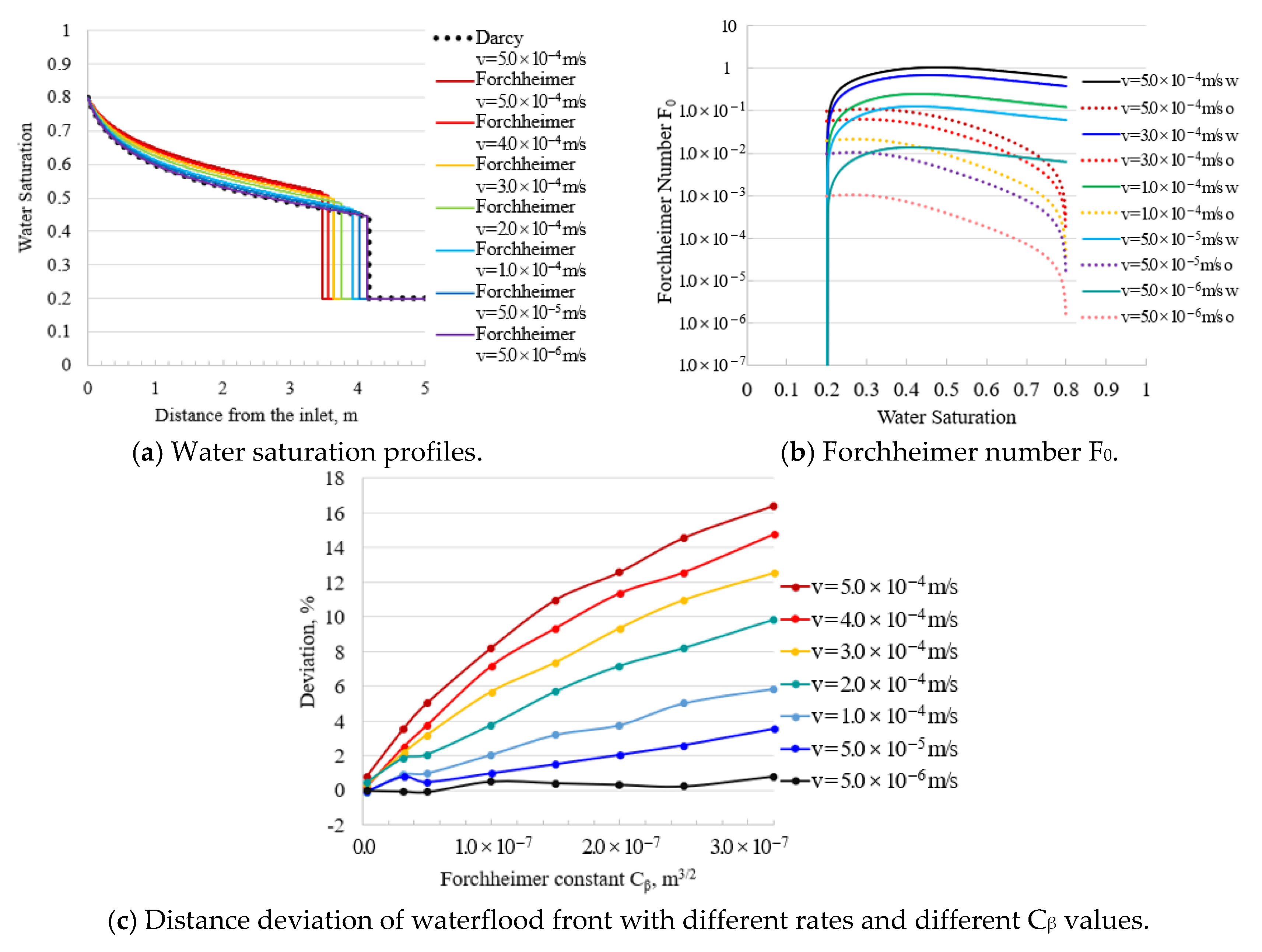
3.1.3. Flow Velocity

When fluids flow in the subsurface, the flow velocity cannot be constant and keeps changing. For instance, the flow velocity is very high near the borehole; as the waterfront advances along the radial direction in the porous media, the flow velocity will gradually decrease. In addition, the velocity may be influenced by the porosity and connectivity. In this section, we will analyze the effect of velocity on non-Darcy behaviors after the same volume of fluids is injected. Here, we assume that the velocity varies from 5.0 × 10⁻⁴ m/s to 5.0 × 10⁻⁶ m/s.

Figure 8 shows the comparison of different flow velocities when C_β equals 3.2 × 10⁻⁷ m^3/2. When the flow velocity is 5.0 × 10⁻⁴ m/s, the sweeping efficiency is the highest and the displacement distance is the shortest. Then, as the velocity decreases, the displacement distance gets longer and becomes close to that of Darcy flow. The values of the Forchheimer number all decrease with a decrease in velocity. When C_β equals 3.2 × 10⁻⁷ m^3/2, most values of the water Forchheimer number are more than 0.01 and those of oil are more than 0.001 when the velocity is larger than 5.0 × 10⁻⁵ m/s. In these cases, the distance deviation of the waterflood front is larger than 0.03 (Figure 8c). When the velocity is no more than 5.0 × 10⁻⁵ m/s, the distance deviation of the waterflood front is less than 0.05, regardless of the C_β value. This means that the inertial force is very small, and the characteristic of the Forchheimer flow is close to that of Darcy flow.

In summary, velocity is the key parameter for the characteristics of fluid flow. When the velocity is larger than a certain value, the non-Darcy effect cannot be ignored, and this threshold value of the velocity is critical. It is much easier to obtain the threshold value of velocity by comparing the distance deviation of the waterflood front than to do so according to the values of the Forchheimer number.

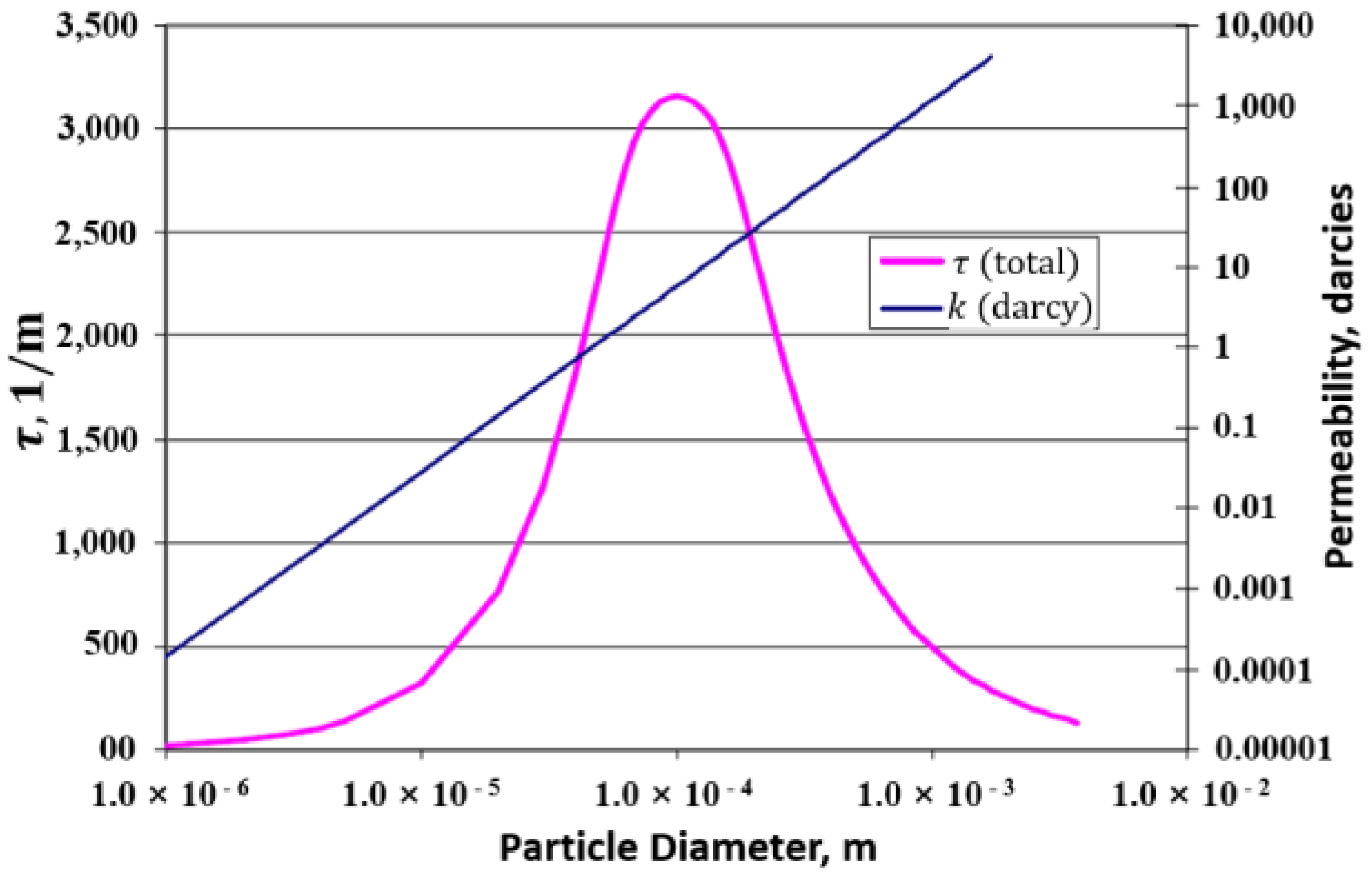
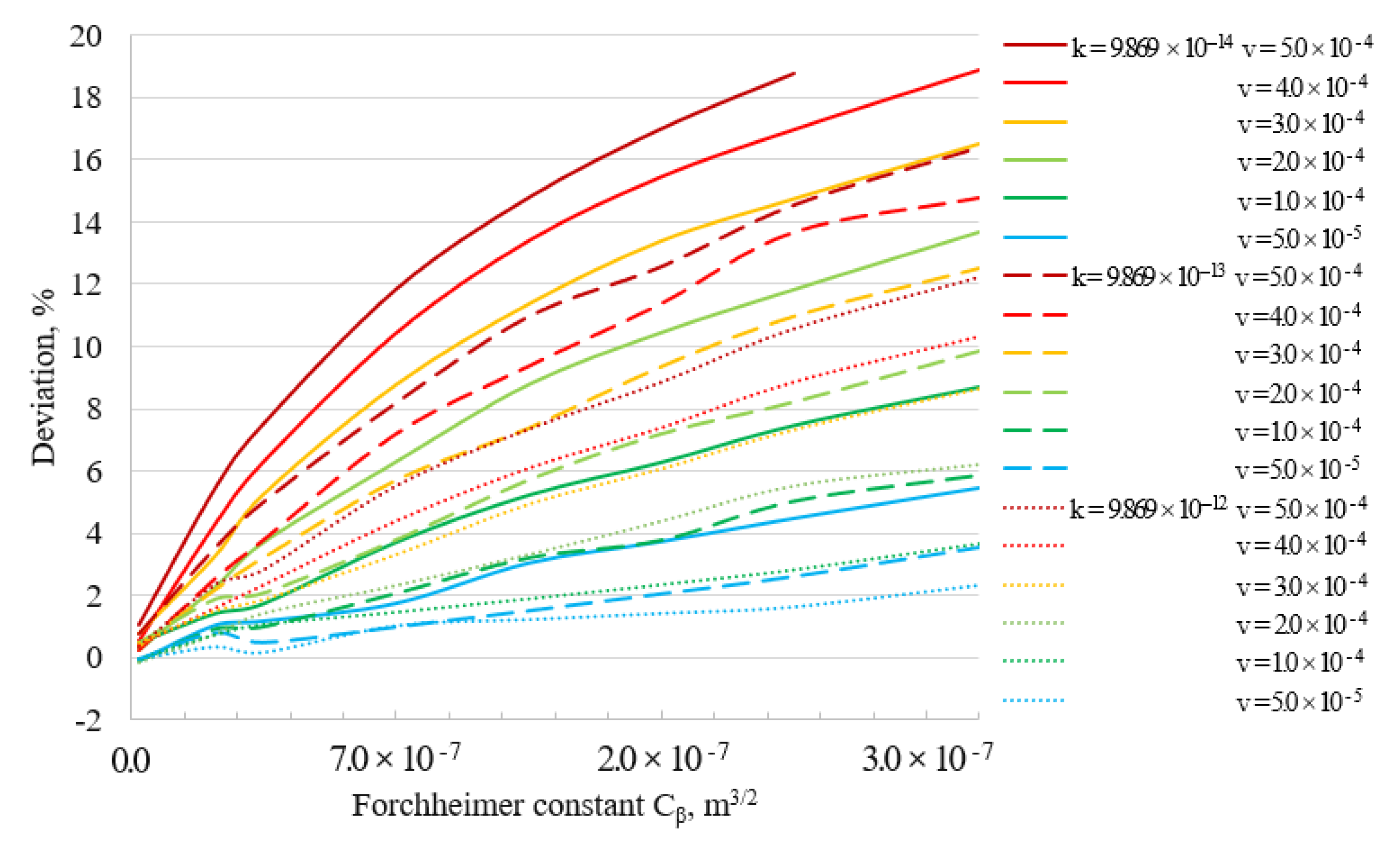
3.1.4. Absolute Permeability

Usually, most reservoirs are heterogeneous and their absolute permeability is not constant. Absolute permeability directly influences the Forchheimer coefficient for non-Darcy flow. In this section, a comparison of the Forchheimer equation with different absolute permeability values will be conducted to evaluate its distance deviations of the waterflood front from Darcy flow. Here, C_β is equal to 1.0 × 10⁻⁷ m^3/2, and the values of absolute permeability are 9.869 × 10⁻¹², 9.869 × 10⁻¹³ and 9.869 × 10⁻¹⁴ m².

Figure 9 shows a comparison of the results of the Darcy and Forchheimer equations with varying absolute permeabilities. According to the water saturation profile (Figure 9a), the displacement distance of waterfront travel is shortest for the lowest absolute permeabilities because of the high flow resistance for the same injection volume. Here, F₀ increases as the absolute permeability decreases (Figure 9b). This means that the lower absolute permeability will enhance the non-Darcy effect and lead to better displacement efficiency. When the absolute permeability is 9.869 × 10⁻¹² m², the distance deviation of the waterflood front between the Forchheimer and Darcy equations is 10.5%. As the absolute permeability decreases, the distance deviation of the waterflood front increases, reaching 20.1% when the absolute permeability is 4.935 × 10⁻¹⁴ m².

In summary, more attention should be paid to the lower absolute permeability region, because lower absolute permeability results in high flow resistance, and the inertial effect increases. Thus, when the fluid flows from high absolute permeability to lower absolute permeability, the flow regime may change from Darcy flow to non-Darcy flow.

3.1.5. Effect of Parameters

As previously stated, there are many factors related to fluids and rock that can affect the inertial force, and the distance deviation of the waterflood front can describe the magnitude of the inertial effect well. In this section, we will set the water viscosity to 0.001 mPa·s to analyze the inertial effect with different Forchheimer constants, absolute permeability and flow velocity. The distribution characteristic and laws of the distance deviation of the waterflood front for waterfront travel under different conditions are shown in Figure 10. When the flow rate is less than 5.0 × 10⁻⁵ m/s, the distance deviation of the waterflood front is less than 6.0% and the non-Darcy effect is insignificant. When the Forchheimer constant is less than 3.2 × 10⁻⁸ m^3/2, the distance deviation of the waterflood front is within 5.0% and the non-Darcy effect can be ignored. In the other cases, the distance deviation of the waterflood front (Figure 10) can assist in determining whether to consider the non-Darcy effect and choosing the suitable flow equation; it can also aid in evaluating the numerical simulation error for a heterogeneous reservoir.

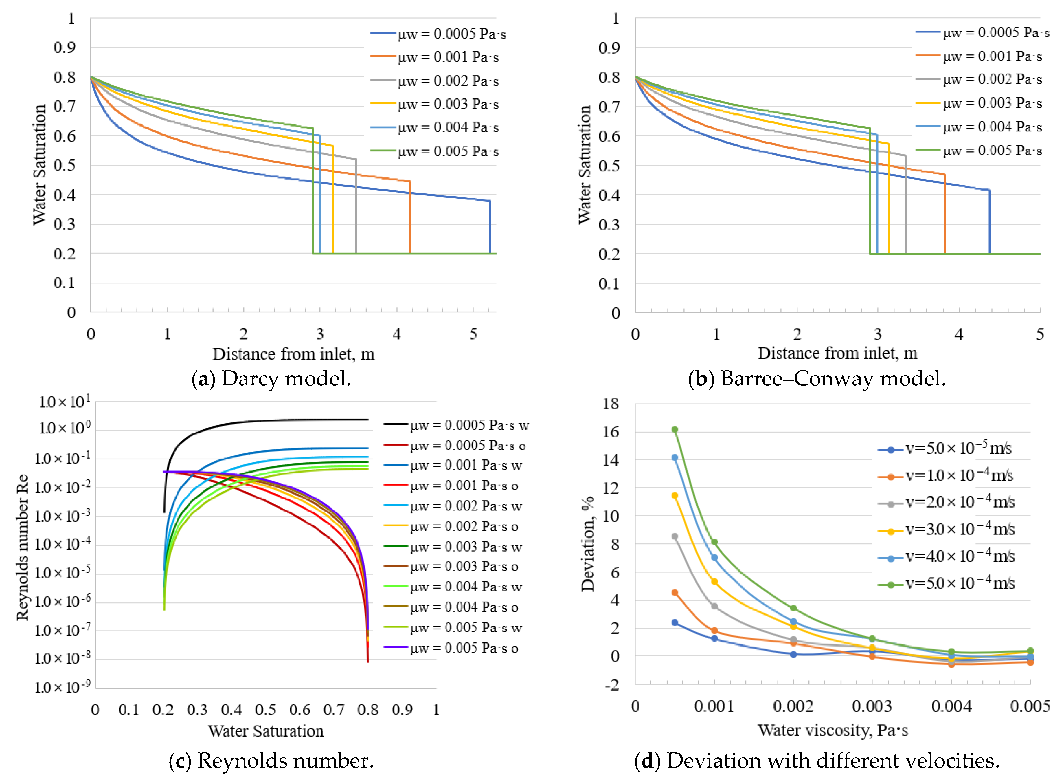
3.2. Comparison of Darcy and Barree–Conway Equations

3.2.1. Fluid Viscosity

Here, we assume that the constant viscosity of oil is 0.005 Pa·s and water viscosity takes the following values: 0.0005, 0.001, 0.002, 0.003, 0.004 and 0.005 Pa·s.

Figure 11 shows the water saturation profiles of the Darcy and Barree–Conway equations for different oil–water viscosity ratios. Similarly, as the oil–water viscosity decreases, the influence of the non-Darcy effect weakens; when the water viscosity is greater than 0.002 Pa·s, the distance deviation of the waterflood front is less than 4% (Figure 11d). When the oil–water viscosity ratio decreases, the Reynolds number of the water decreases, whereas that of the oil increases (Figure 11c). We cannot evaluate the non-Darcy effect only according to the Forchheimer numbers of the water and oil phases. The distance deviations of the waterflood front with different flow rates are shown in Figure 11d. Even when the flow rate is very high (v = 5.0 × 10⁻⁴ m/s) and the water viscosity is no less than 0.002 Pa·s, the distance deviation of the waterflood front is less than 4.0%, indicating that the non-Darcy effect is insignificant. When the oil–water viscosity ratio is extremely high, the non-Darcy effect increases as the flow rate increases.

3.2.2. Flow Velocity

In this section, we will analyze the effect of velocity on the non-Darcy behavior for the same porous media, assuming that the water viscosity is 0.001 Pa·s and the velocity varies from 5.0 × 10⁻⁴ m/s to 5.0 × 10⁻⁵ m/s.

Figure 12 shows the comparison of different flow velocities. When the flow rate is 5.0 × 10⁻⁴ m/s, the sweeping efficiency is the highest and the displacement distance is the shortest for the same porous media. Thereafter, as the rate decreases, the displacement distance increases and comes close but does not overlap with that of Darcy flow; the distance deviation of the waterflood front still is greater than 1% even when the flow rate is 0.5 × 10⁻⁴ m/s (Figure 12c), and the values of Reynolds number all decrease as the flow rate decreases. When the flow rate is less than 2.0 × 10⁻⁴ m/s, the distance deviation of the waterflood front is less than 4% and the Reynolds number is still within several orders of magnitude. In summary, velocity is still the critical parameter in the Barree–Conway model. When the velocity is less than a certain value, the distance deviation of the waterflood front is significantly small, and the non-Darcy effect can be ignored; however, the Reynolds number is not a constant value and will be within several orders of magnitude.

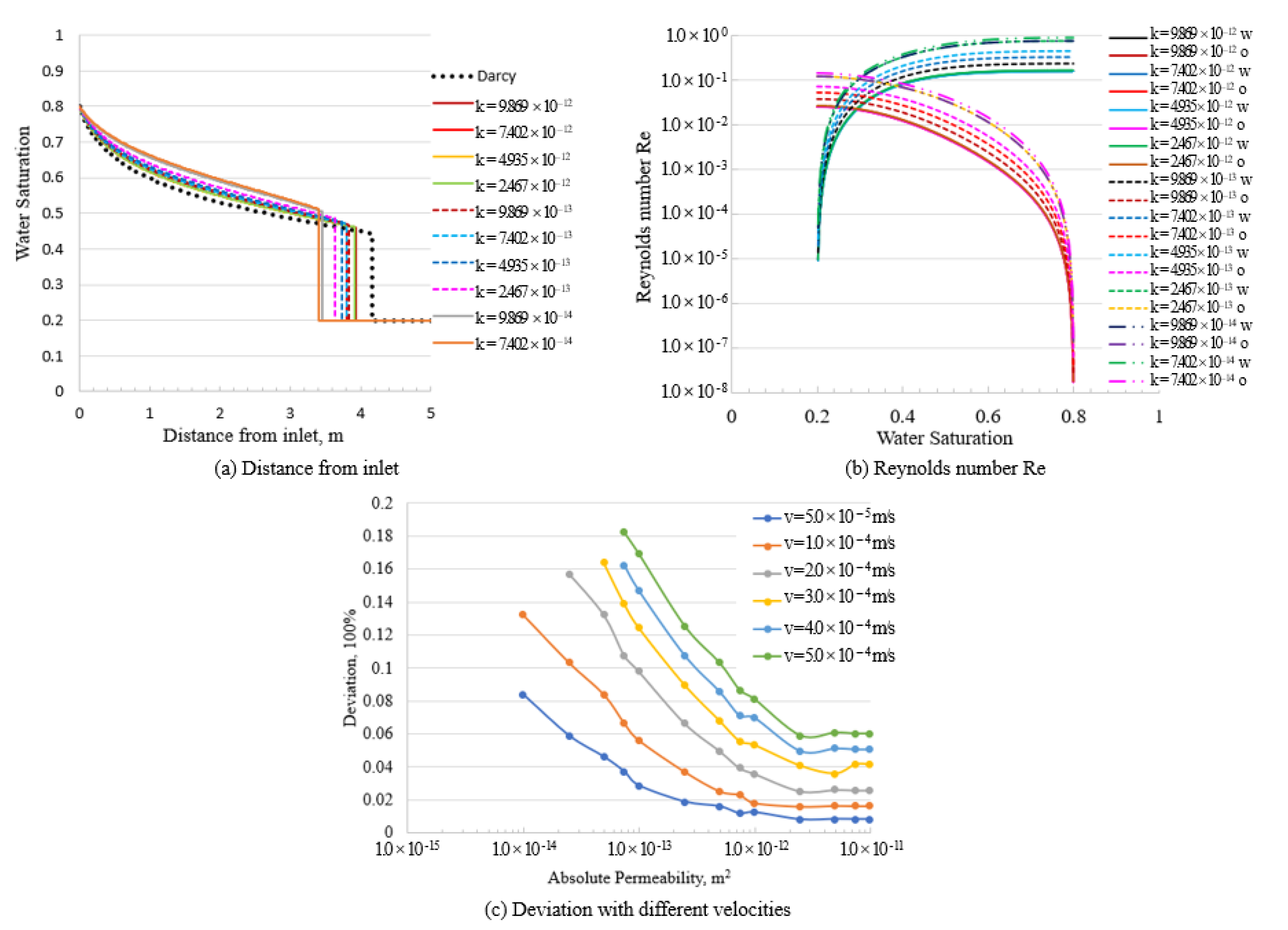
3.2.3. Absolute Permeability

The results of the Barree–Conway model with different absolute permeabilities will be compared in this section to evaluate the distance deviations of the waterflood front with respect to Darcy flow. Here, the absolute permeability value ranges from 9.869 × 10⁻¹² to 7.402 × 10⁻¹⁴ m² and the value of τ is obtained using the relationship in Figure 2 (

Table 2. Parameter of Barree–Conway model (Figure 2).

	Absolute Permeability k, m2	Inverse of Characteristic Length τ, m−1
1	9.869 × 10−12	3100
2	7.402 × 10−12	3100
3	4.935 × 10−12	3150
4	2.467 × 10−12	3000
5	9.869 × 10−13	2100
6	7.402 × 10−13	1900
7	4.935 × 10−13	1500
8	2.467 × 10−13	1100
9	9.869 × 10−14	650
10	7.402 × 10−14	550

).

Figure 13 shows the comparison results of the Darcy and Barree–Conway models with various absolute permeabilities when the flow velocity is 5.0 × 10⁻⁴ m/s. According to the water saturation profile (Figure 13a), the displacement distance of waterfront travel is shortest for the lowest absolute permeabilities with the same injection volume, and the distance deviation of the waterflood front decreases as the absolute permeability increases. When the absolute permeability is greater than 2.467 × 10⁻¹² m², the distance deviation of the waterflood front remains around 6% because there is little difference in the value of another key parameter, τ (Table 2). The Reynolds number decreases as the absolute permeability increases (Figure 13b). The distance deviation of the waterflood front decreases as the flow rate decreases (Figure 13c). For the same flow rate, the absolute permeability increases from 2.467 × 10⁻¹² m² to 9.869 × 10⁻¹² m², while the distance deviation of the waterflood front is kept nearly constant because the value of τ is almost the same.

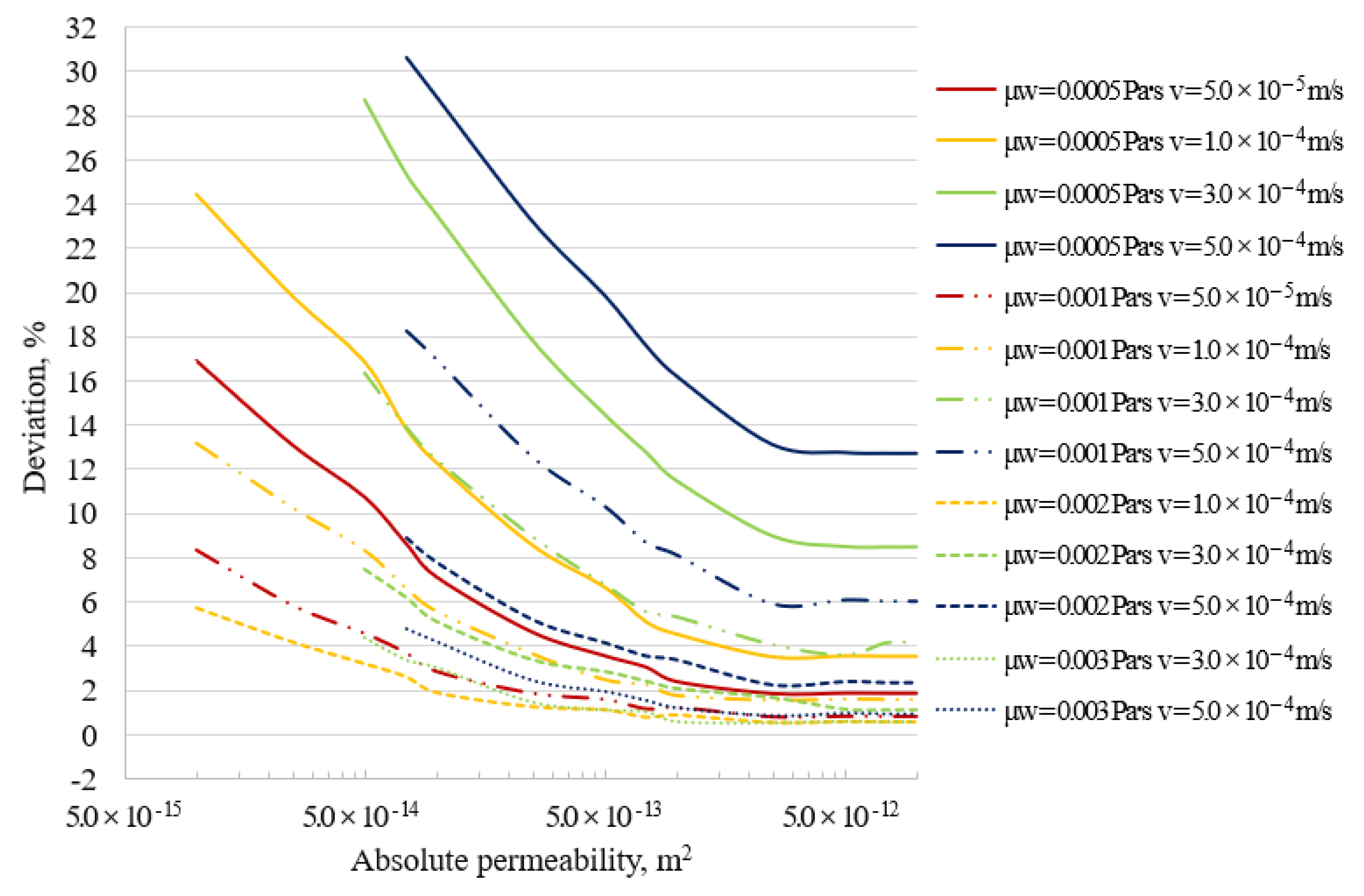
3.2.4. Effect of Parameters

The parameters relating to fluids and rock influence the non-Darcy effect, and the distance deviation of the waterflood front can directly describe the magnitude of the non-Darcy effect. In this section, we will set the oil viscosity to 0.005 Pa·s and analyze the non-Darcy effect with different water viscosities, absolute permeabilities, and flow rates (Figure 14). When the water viscosity is greater than or equal to 0.004 Pa·s, the distance deviation of the waterflood front is less than 3%; when the water viscosity is greater than or equal to 0.003 Pa·s, the distance deviation of the waterflood front is less than 5% and the non-Darcy effect still is not evident; when the water viscosity is equal to 0.002 Pa·s, the non-Darcy effect cannot be ignored in cases with a high flow rate in the low permeability area; when the viscosity ratio of oil–water is extremely large (μ_o = 0.005 Pa·s and μ_w = 0.0005 Pa·s), the distance deviation of the waterflood front is evident and the inertial effect cannot be ignored, especially for a high flow rate and low absolute permeability. The distribution of the distance deviation of the waterflood front with the different parameters is shown in Figure 14.

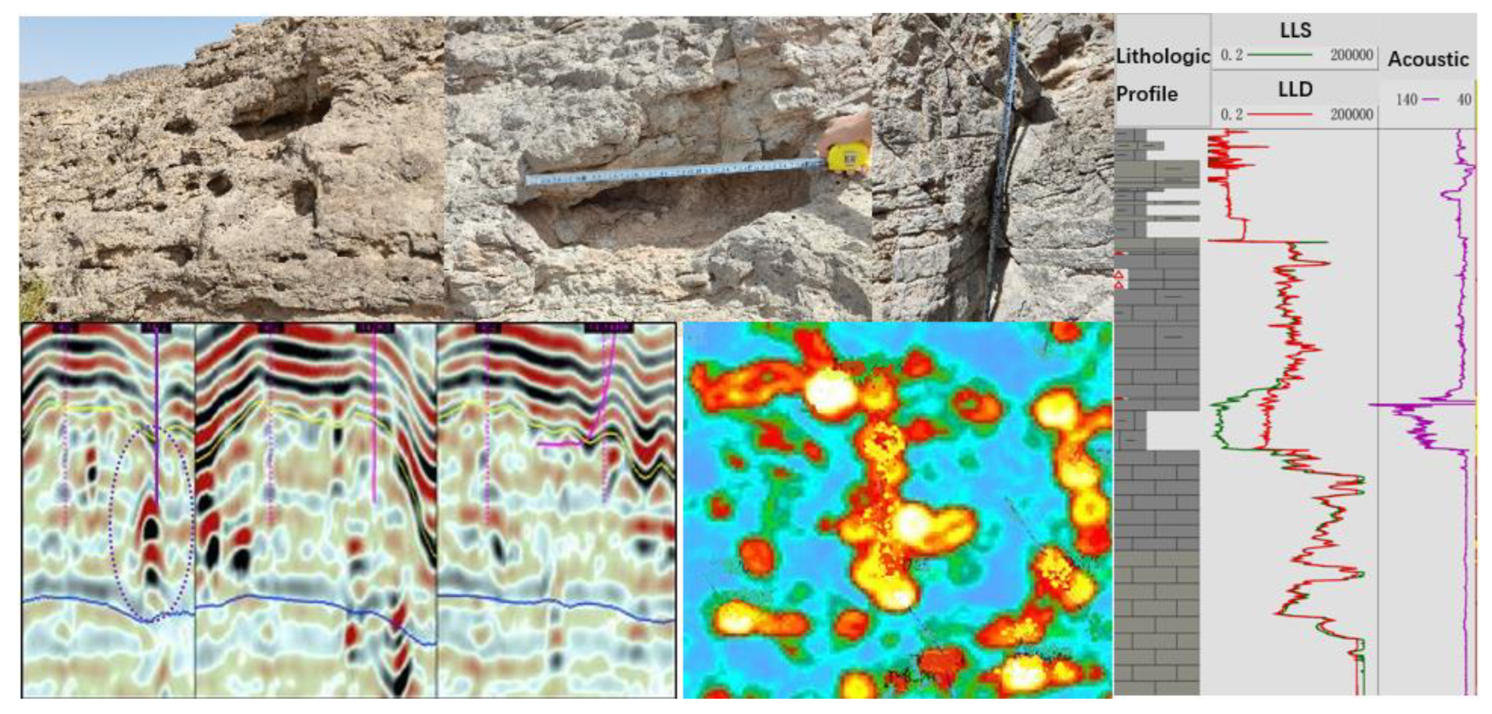
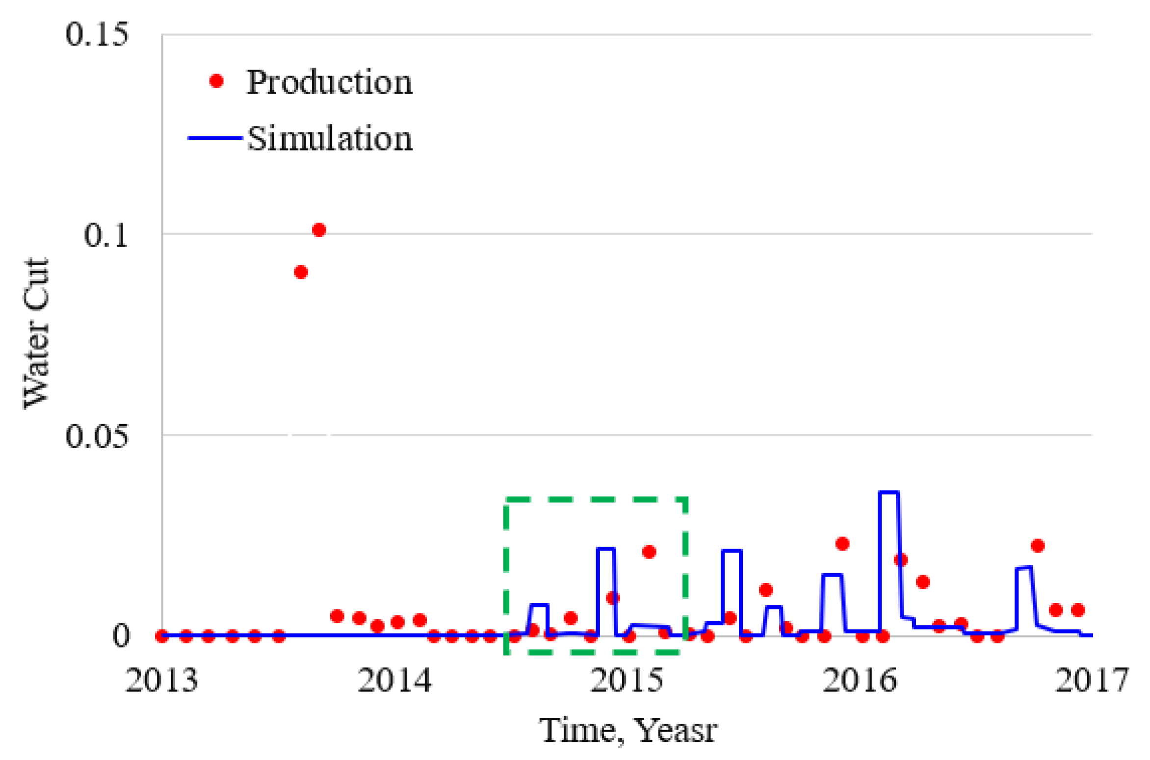
4. Applications of Tarim Fractured Karstic Carbonate Reservoir

We used this method to analyze the distance deviation of the waterflood front at the fractured karstic region in the Tarim reservoir. We chose one well area developing fractures and karstic caves, which were verified from the logging curves, seismic profiles and obtained cores (Figure 15). There were obvious signs of karstic caves and fractures in the seismic profiles and logging curves, and it was hard to obtain a core from the target strata. According to the geophysical method, the average porosity of underground reservoirs is widely distributed: about 2.0% in the low porosity area and up to 50% in the dissolution pores and karstic cave areas. The average permeability varies from 4.93 × 10⁻¹³ m² to 9.869 × 10⁻¹¹ m². According to previous exploration and developments, the production well is located in the fracture cave regions, the porosity is about 45% and the initial effective permeability is 4.93 × 10⁻¹³ m². The oil viscosity is 0.05 Pa·s and the density is 860 kg/m³. The water viscosity is 0.0005 Pa·s, and the density is 1000.0 kg/m³. The daily production is about 300.0–500.0 m³, which is clearly a high flow rate; thus, it is a high yield well.

The Eclipse software based on Darcy flow was used to simulate the fluid flows. The geological model was established according to seismic data and logging data, and the fracture and karstic cave development area was finely carved. The karstic cave area was set with high porosity and high permeability according to the seismic data and logging data, and the model was discretized by a 20 m × 20 m × 20 m grid. The well’s conditions were set according of the well performance data, then a numerical simulation using the Eclipse software was carried out from 2013 to 2017. Usually, the next step is to modify the geological model for historical fitting according to the production dynamics. We analyzed the production curves of this production well (Figure 16) before modifying the geological model. The red dotted line is the actual production curve, and the blue line is the result of the numerical simulation using the Eclipse software. Figure 16 shows the difference between them on the production well, especially in the green dotted area. There was an obvious deviation of the water breakthrough time between them on the production well, and the time of water appearance in the numerical simulation was obviously earlier than that in the actual production. The water began to occur around the year 2015 in the actual production curves; however, the time of water appearance was obviously earlier in the numerical simulation using the Darcy equation. The flow velocity calculated by the numerical simulation was greater than the actual flow velocity because the inertial force was ignored; as a result, the water appeared earlier in the numerical simulation than in the actual production. Usually, we do not take the inertial effect into account and directly modify the geological model or phase permeability curve to achieve the historical fitting.

We selected a region within 500.0 m of this production well and used the method described in this paper to analyze the distance deviation of the waterflood front. Since the main storage space was made up of fractures, karst cracks and dissolution pores, the flow rate was set to 5.0 × 10⁻⁵ m/s. Since there was no non-Darcy flow equation parameter determined by the physical experiment, we used the mild values (the large parameter value indicates that the inertial effect is strong, while the small value indicates that the inertial effect can be ignored). We assumed that the Forchheimer constant C_β was equal to 3.2 × 10⁻⁸ m^3/2 and τ was equal to 1500 m⁻¹ in the Barree–Conway equation (Barree and Conway, 2004); these two values describe non-Darcy flow in which the inertial effect is not very strong. The waterflood displacement front and water saturation distribution curves were obtained by the three equations after injecting the same volume multiple times (as shown in Figure 17).

Figure 17 shows that the waterflood frontal movement of Darcy flow was fast and the displacement distance of waterfront travel was the longest once the inertial effect was ignored, and the results of non-Darcy flow considering inertia were obviously different from those of Darcy flow. The distance deviation of the waterflood front was 4.69% using the Forchheimer equation and 5.04% using the Barree–Conway equation. The inertial effect should be one of the important factors, although there are many factors affecting the time of water emergence. With the reservoir developing, the distance deviation of the waterflood front between the simulation and the actual production ignoring the inertial effect will increase, thus further affecting the modification of the geological model, historical fitting and yield prediction. In reservoir development research, it is generally accepted that geological parameters are modified to achieve consistency in the dynamic production curve, then the prediction of future development dynamics is performed. Here, the geological model and the actual reservoir were equivalent models based on different flow states. In other words, a geological model based on Darcy flow is equivalent to an actual reservoir based on non-Darcy flow, which will lead to further errors in subsequent oil and gas field development and the prediction of remaining oil.

5. Conclusions

Several conclusions can be drawn from the comparison and analysis carried out in this paper:

• It is not very realistic that the non-Darcy flow equation is used to simulate fluid flow in fractured karstic carbonate reservoirs. It is the inertial term in Forchheimer model and the apparent permeability in the Barree–Conway model that make these equations more complex than the Darcy equation. Furthermore, it will dramatically increase the difficulty and expense of numerical simulation.
• The Forchheimer number and Reynolds number do not quantify the magnitude of the inertial effect. In addition, the crucial values of the Forchheimer number and Reynolds number are not constant and vary with the parameters of the rock and fluid properties. It is very difficult to determine whether to consider the non-Darcy effect only according to the Forchheimer/Reynolds number.
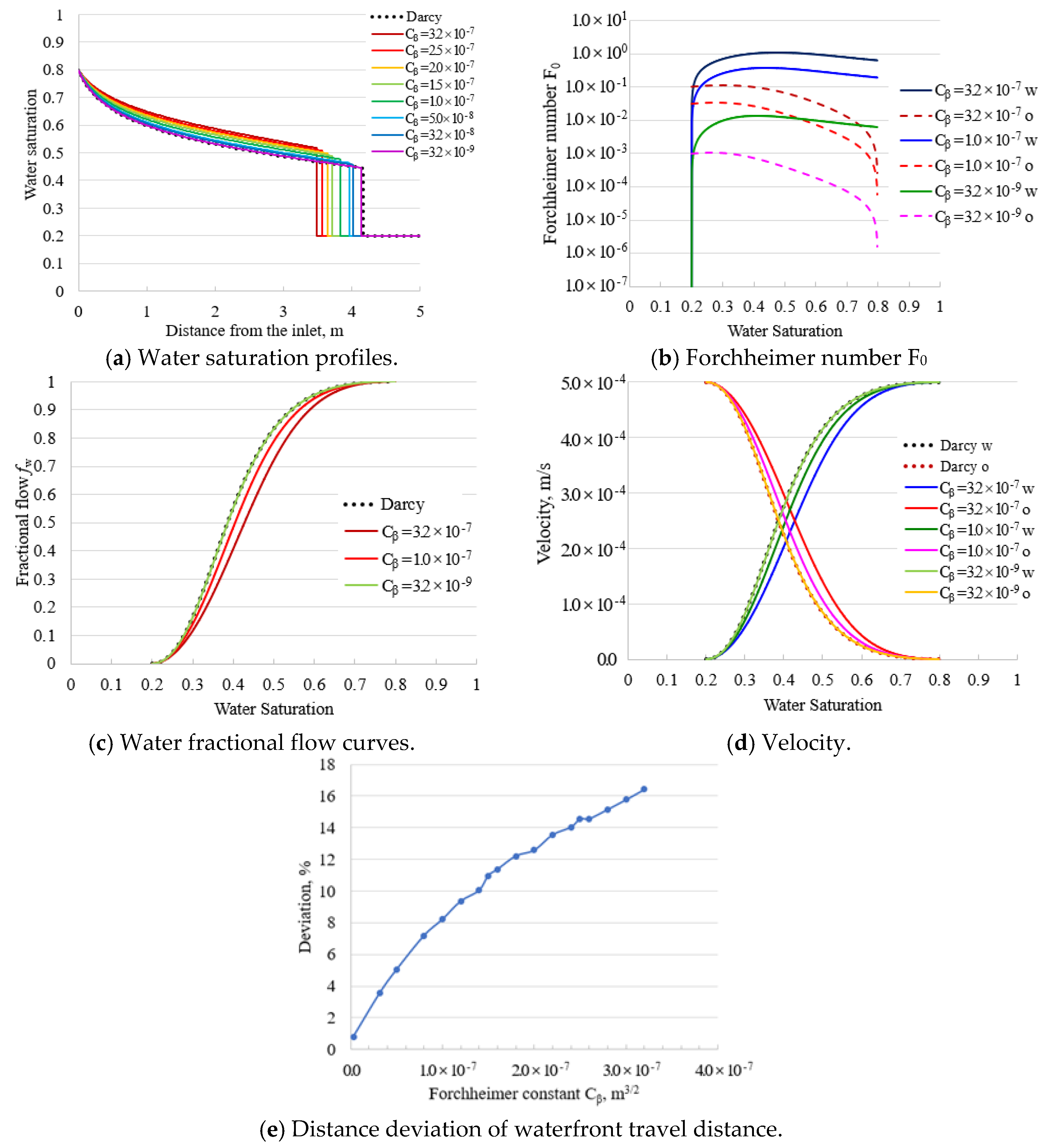
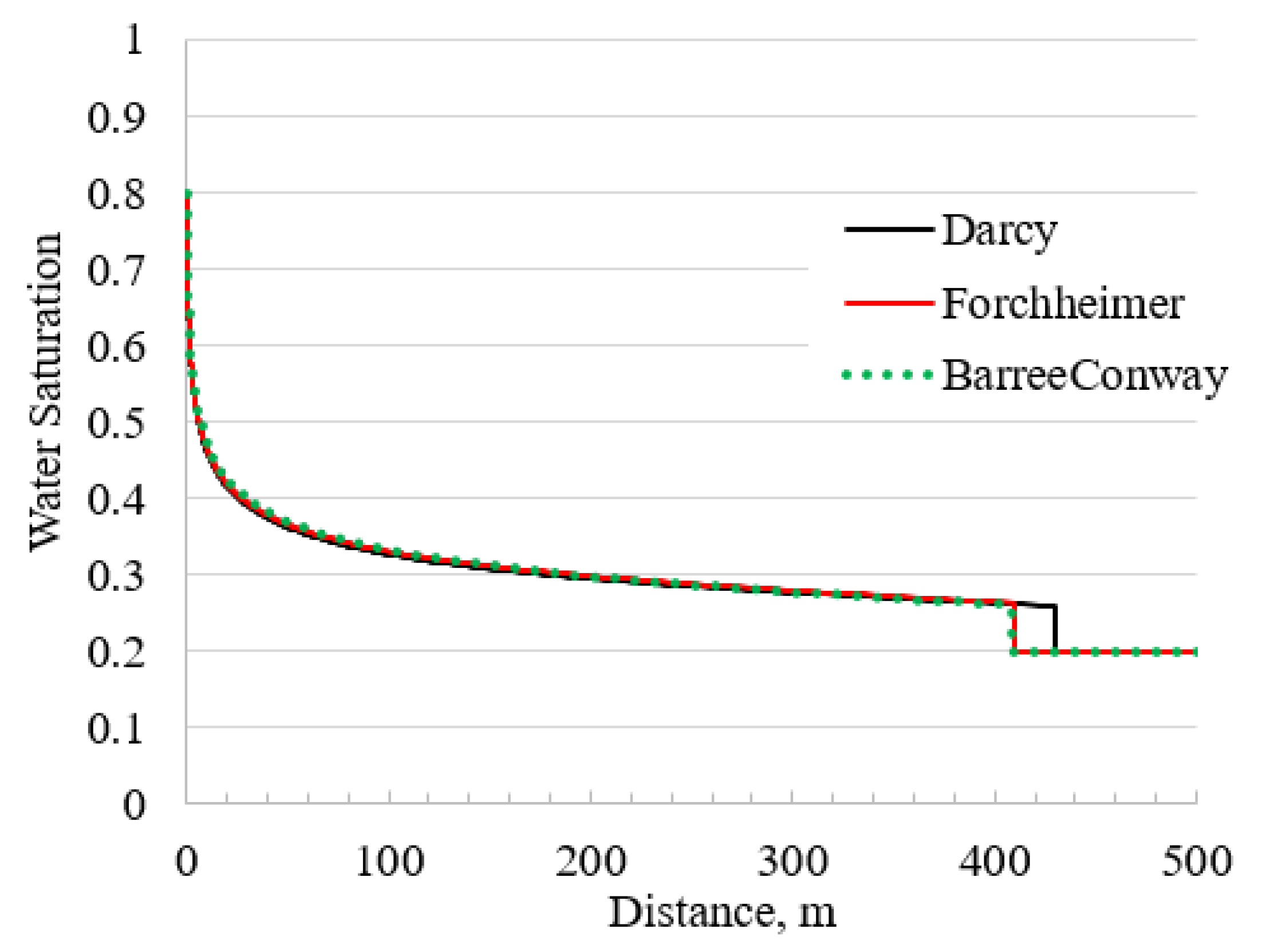
• The distance deviation of the waterflood front can better describe the inertial effect of multiphase flow. In numerical simulation, we are concerned with the displacement range and the sweeping efficiency. According to the distance deviation of the waterflood front between the Darcy and non-Darcy equations, we will not only choose the flow equation within the numerical error allowed, but also obtain the evaluation of the numerical error for a complex heterogeneous reservoir.

References

1. Akbar, M.; Vissapragada, B.; Alghamdi, A.H. A snapshot of carbonate reservoir evaluation. Oilfield Rev. 2000, 12, 20–21. [Google Scholar]
2. Srinivasan, S.; O’Malley, D.; Mudunuru, M.K. A machine learning framework for rapid forecasting and history matching in unconventional reservoirs. Sci. Rep. 2021, 11, 21730. [Google Scholar] [CrossRef] [PubMed]
3. Yao, J.; Sun, H.; Li, A. Modern System of multiphase flow in porous media and its development trend. Sci. China Press 2018, 63, 425–451. [Google Scholar] [CrossRef] [Green Version]
4. Darcy, H. Les Fontaines Publiques de la Ville de Dijon; Technical Report; Dalmont: Paris, France, 1856. [Google Scholar]
5. Forchheimer, P. Wasserbewegung durch boden. Z. Ver Deutsh. Ing. 1901, 45, 1782–1788. [Google Scholar]
6. Whitaker, S. Advances in theory of fluid motion in porous media. Ind. Eng. Chem. 1969, 61, 14–28. [Google Scholar] [CrossRef]
7. Jones, S.C. A Rapid Unsteady-State Klinkenberg Permeameter. Soc. Pet. Eng. J. 1972, 12, 383–397. [Google Scholar] [CrossRef]
8. Geertsma, J. Estimating the Coefficient of Inertial Resistance in Fluid Flow through Porous Media. Soc. Pet. Eng. J. 1974, 14, 445–450. [Google Scholar] [CrossRef]
9. Firoozabadi, A.; Katz, D.L. An analysis of high-velocity gas flow through porous media. J. Petrol. Technol 1979, 31, 211–216. [Google Scholar] [CrossRef]
10. Ruth, D.; Ma, H. On the derivation of the Forchheimer equation by means of the averaging theorem. Transp. Porous Media 1992, 7, 255–264. [Google Scholar] [CrossRef]
11. Barree, R.D.; Conway, W. Beyond Beta Factors: A Complete Model for Darcy, Forchheimer, and Trans-Forchheimer Flow in Porous Media. In Proceedings of the SPE Annual Technical Conference and Exhibition (SPE 2004), Houston, TX, USA, 26–29 September 2004; pp. 1–8. [Google Scholar]
12. Barree, R.D.; Conway, M.W. Multiphase non-darcy flow in proppant packs. In Proceedings of the SPE Annual Technical Conference and Exhibition (SPE 2007), Anaheim, CA, USA, 11–14 November 2007; pp. 1–10. [Google Scholar]
13. Chilton, T.H.; Colburn, A.P. Pressure drop in packed tubes. Ind Engng. Chem. 1931, 23, 913–919. [Google Scholar] [CrossRef]
14. Green, L., Jr.; Duwez, P. Fluid flow through porous metals. J. Appl. Mech. 1951, 18, 39–45. [Google Scholar] [CrossRef]
15. Ma, H.; Ruth, D.W. The microscopic analysis of high Forchheimer number flow in porous media. Transp. Porous Media 1993, 13, 139–160. [Google Scholar] [CrossRef]
16. Ergun, S. Fluid flow through packed columns. Chem. Engng. Prog. 1952, 48, 89–94. [Google Scholar]
17. Evans, R.D.; Hudson, C.S.; Greenlee, J.E. The effect of an immobile liquid saturation on the non-darcy flow coefficient in porous media. SPE Prod. Eng. 1987, 2, 331–338. [Google Scholar] [CrossRef]
18. Scheidegger, A.E. The Physics of Flow through Porous Media, 3rd ed.; University of Toronto Press, Scholarly Publishing: Toronto, ON, Canada, 1974; pp. 31–150. [Google Scholar]
19. Blick, E.F.; Civan, F. Porous media momentum equation for highly accelerated flow. SPE Reserv. Engng. 1988, 3, 1048–1052. [Google Scholar] [CrossRef]
20. Bear, J. Hydraulics of Groundwater; McGraw-Hill: New York, NY, USA, 1979; pp. 66–82. [Google Scholar]
21. Wu, Y. Non-Darcy displacement of immiscible fluids in porous media. Water Resour. Res. 2001, 37, 2943–2950. [Google Scholar] [CrossRef]
22. Bitao, L.; Jennifer, L.; Wu, Y.-S. Non-darcy porous media flow according to the barree and conway model: Laboratory and numerical modeling studies. In Proceeding of the SPE Rocky Mountain Petroleum Technology Conference (SPE 2009), Denver, CO, USA, 14–16 April 2009; pp. 1–10. [Google Scholar]
23. Brooks, R.H.; Corey, A.T. Hydraulic Properties of Porous Media. In Hydrology Papers; Colorado State University: Fort Collins, CO, USA, 1964. [Google Scholar]
24. Zhengwen, Z.; Reid, G. A criterion for Non-Darcy Flow in Porous Media. Transp. Porous Media 2006, 63, 57–69. [Google Scholar]
Figure 1. Relationship between pressure gradient and velocity.
Energies 15 03623 g001
Figure 2. τ and permeability related to mean particle size (Barree, 2004) [11].
Energies 15 03623 g002
Figure 3. Comparison of Darcy, Forchheimer and Barree–Conway equations. (a) Water saturation profiles. (b) Velocity. (c) Water fractional flow curves. (d) Forchheimer number of Forchheimer equation and Reynolds number of Barree–Conway equation.
Energies 15 03623 g003
Figure 4. Forchheimer coefficient curves.
Energies 15 03623 g004
Figure 5. Comparison of Darcy equation versus Forchheimer equation with different Cβ values.
Energies 15 03623 g005
Figure 6. Water saturation profiles of Darcy versus Forchheimer flow with different fluid viscosities.
Energies 15 03623 g006
Figure 7. Forchheimer number F0 of Forchheimer flow with different fluid viscosities.
Energies 15 03623 g007
Figure 8. Comparison of Darcy flow versus Forchheimer flow at different flow rates.
Energies 15 03623 g008
Figure 9. Comparison of Darcy vs. Forchheimer equations with various absolute permeabilities.
Energies 15 03623 g009
Figure 10. Distance deviation of waterflood front with various parameters.
Energies 15 03623 g010
Figure 11. Comparison of Darcy model versus Barree–Conway model for different water viscosities.
Energies 15 03623 g011
Figure 12. Comparison of Darcy model vs. Barree–Conway model for different flow velocities.
Energies 15 03623 g012
Figure 13. Comparison of Darcy model versus Barree–Conway model for different flow velocities.
Energies 15 03623 g013
Figure 14. Distance deviation of Darcy equation versus Barree–Conway equation.
Energies 15 03623 g014
Figure 15. Geology and geophysics response of fractured karstic carbonate rocks.
Energies 15 03623 g015
Figure 16. Results of production and numerical simulation.
Energies 15 03623 g016
Figure 17. Displacement distance of waterfront travel.
Energies 15 03623 g017