Self-Supervised Railway Surface Defect Detection with Defect Removal Variational Autoencoders

Abstract

In railway surface defect detection applications, supervised deep learning methods suffer from the problems of insufficient defect samples and an imbalance between positive and negative samples. To overcome these problems, we propose a lightweight two-stage architecture including the railway cropping network (RC-Net) and defects removal variational autoencoder (DR-VAE), which requires only normal samples for training to achieve defect detection. First, we design a simple and effective RC-Net to extract railway surfaces accurately from railway inspection images. Second, the DR-VAE is proposed for background reconstruction of railway surface images to detect defects by self-supervised learning. Specifically, during the training process, DR-VAE contains a defect random mask module (D-RM) to generate self-supervised signals and uses a structural similarity index measure (SSIM) as pixel loss. In addition, the decoder of DR-VAE also acts as a discriminator to implement introspective adversarial training. In the inference stage, we reduce the random error of reconstruction by introducing a distribution capacity attenuation factor, and finally use the residuals of the original and reconstructed images to achieve segmentation of the defects. The experiments, including core parameter exploration and comparison with other models, indicate that the model can achieve a high detection accuracy.

1. Introduction

Recently, with the increase of railways operating mileage and railway loads, the surface defects of rails have also increased. Therefore, the issue of classification, detection and segmentation of rail surface defects has received considerable critical attention [1]. Among the traditional methods, Yu et al. [2] employed phase Fourier and multiscale features for rail surface defect detection. A coarse-to-fine feature extractor [3] was used to gradually extract defects based on the mean shift and saliency map reported. Rail surface defects are detected by Ni et al. [4] with center-point estimation. By reducing the imbalance between negatives and positives, the method of [5] optimized the performance of detection. Yaman et al. [6] proposed a fuzzy classification method for rail surface fault diagnosis. However, most of the above methods are limited by manual feature extraction or sample imbalance and are susceptible to variable defect patterns, as well as complex backgrounds. With the gradual maturity of supervised methods based on deep learning, both in theoretical and practical uses, their application to rail surface defect detection problems has been significantly improved [7,8]. However, a lot of labeled data is needed for training to guarantee the performance of the models, which makes the labor cost of preparing the data much higher. Meanwhile, there is a serious imbalance between normal rail surface data and defective data, which limits the application of supervised methods. Therefore, reducing the labor cost, while ensuring the detection accuracy, remains a very significant issue.

Over the past few years, several research fields have recognized the benefits of anomaly detection. Unlike traditional defect detection, some anomaly detection methods first learn the latent distribution of defect-free samples, which describes the main information of normal samples, and then discriminate anomalies based on the probability that a test sample belongs to the learned latent distribution. An anomaly detection method is flexible and it can be applied to different fields by simply adjusting the reconstruction and anomaly scoring strategies [9]. Moreover, only defect-free samples are used to train them.

Anomaly detection has received a great deal of attention as a method for identifying unexpected data in many applications., such as video surveillance [10], data security [11] and defect detection [12,13]. In addition, strategies generally include unsupervised clustering, high-dimensional spatial classification and evaluation of the reconstruction quality. Xiong et al. [14] proposed an unsupervised clustering method to achieve anomaly detection. In [15], the authors expected to find a hyperplane to distinguish normal samples from anomalous ones. However, the performance efficiency of the above strategy is limited by its feature representation and classification capability. Another strategy is to distinguish anomalies by reconstruction errors or divergence of potential distributions [16,17,18], which has achieved excellent results in certain fields. Relying on adversarial training, Akcay et al. [19] achieved anomaly detection with a latent space feature. Medel et al. [20] proposed predictive convolutional long- and short-term memory networks for anomaly detection. With the proposal of generative adversarial networks, scholars have proposed various models including OCGAN (one-class GAN) [21], AnoGAN [22] and ALAD (adversarial learning anomaly detection) [23], which explicitly restricts the latent space in the expectation of a more robust performance. Other studies [24,25], using a memory enhancement method, dealt with the problem of excessive generalization of the decoder.

However, the following challenges remain on rail surface defect detection: (i) The contrast between some defective pixels and the background is small and makes it easy for defects to be misidentified as background. (ii) The background of the normal rail surface varies greatly depending on the railway operating conditions (load, environment etc.). (iii) In an industrial environment, the image acquisition process is almost unaffected because it can be controlled manually in a very stable way. However, rails are mostly installed in outdoor environments where there are many factors (light, dust, rust, etc.) that affect image acquisition, resulting in unstable image quality such as contrast, grayscale uniformity, noise interference and false defect targets, etc.

To overcome the above difficulties, inspired by the idea of self-supervised learning and Soft-IntroVAE [26], we proposed a two-stage rail surface defect detection system based on the rail surface cropping network (RC-Net) and defect removal autoencoder (DR-VAE). The system first locates and extracts the rail surface from the original image of the rail inspection vehicle by RC-Net, then it segments the defects and detects anomalies using the DR-VAE inference network. The contributions of this paper are summarized as follows:

• We designed the RC-Net based on the feature complexity of railway inspection images, which greatly simplifies the model parameters, while ensuring rail surface detection accuracy.
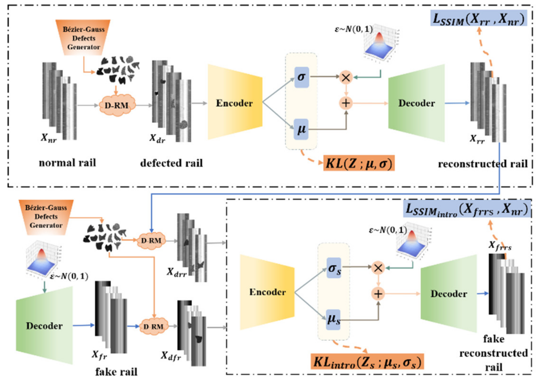
• A self-supervised rail surface defect detection model based on DR-VAE is proposed with a structural similarity index measure (SSIM) [27] and introspective variational autoencoder structure, which avoids additional discriminators and simplifies the network structure, while improving the background reconstruction accuracy using adversarial training.
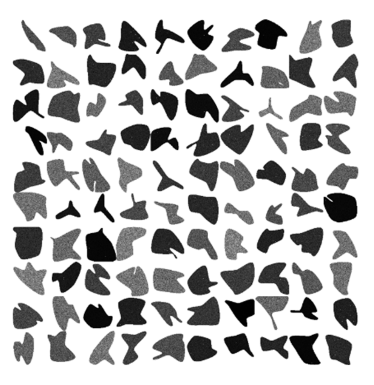
• A defect random mask (D-RM) module is applied to normal rail surfaces during the training process, which provides self-supervised data to improve the defect removal capability of the encoder when reconstructing the background.
• A distribution capacity attenuation factor is proposed in the testing phase to limit the sampling range of the decoder from the latent space, thus reducing the randomness of reconstruction during inferencing and suppressing the problem of excessive generalization of the autoencoder.

2. Materials and Methods

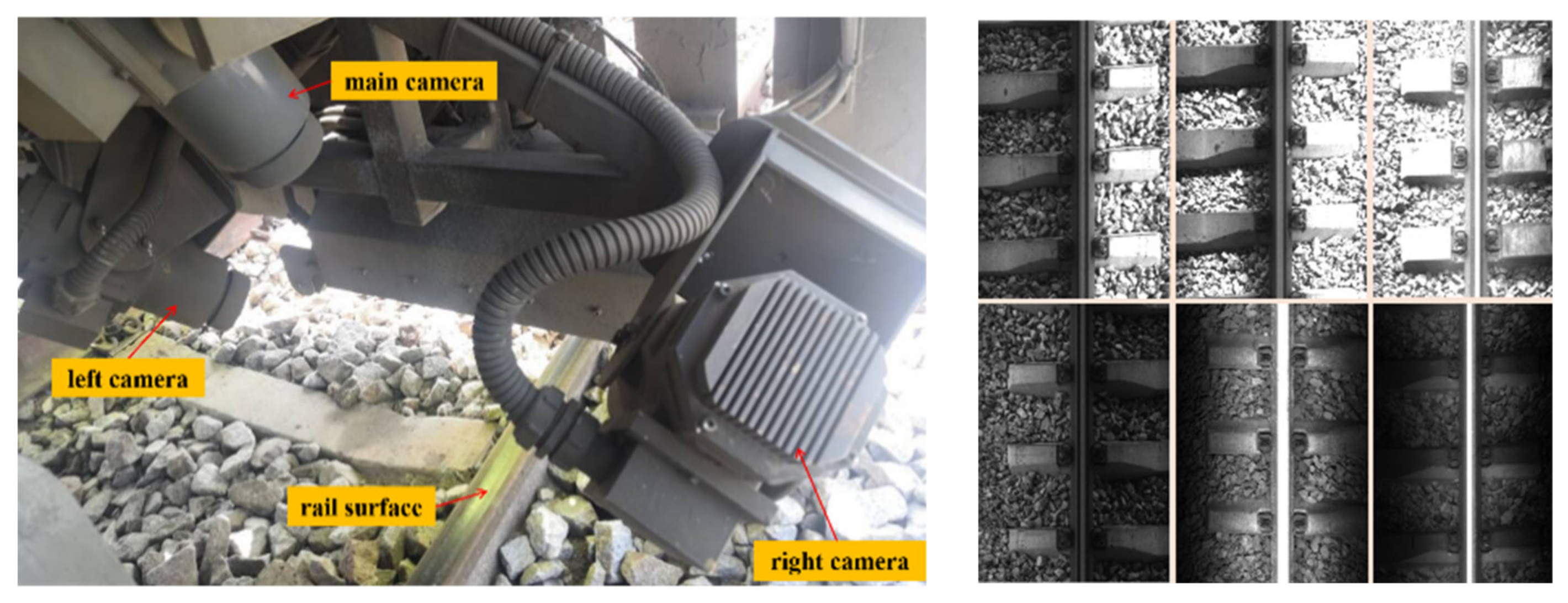
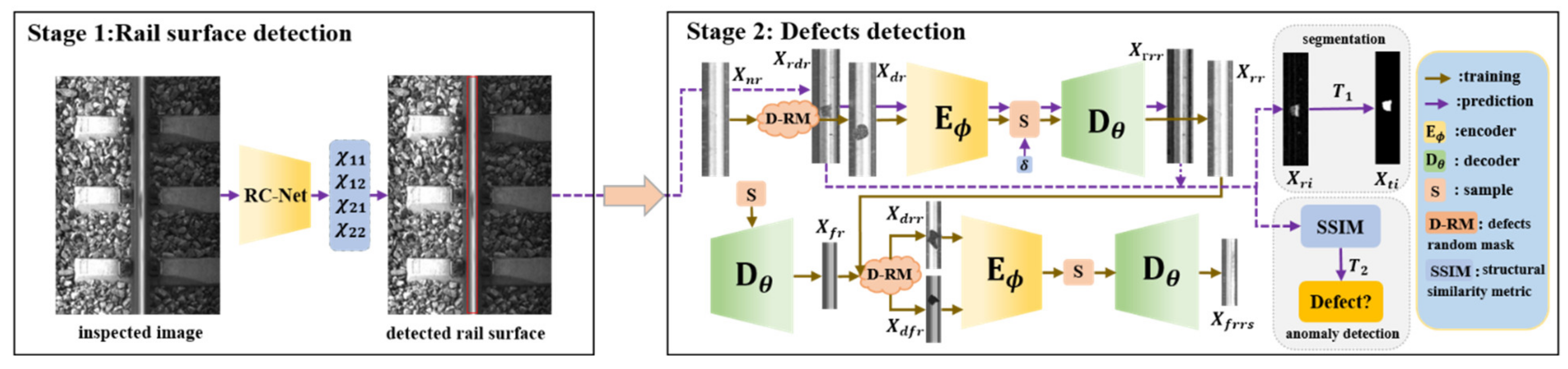
2.1. System Overview

The image acquisition system of the rail inspection car includes three groups of cameras and auxiliary lighting devices, installed at the bottom of the inspection vehicle. The cameras take images of the rail surface from the top, left and right, and the acquisition system stores its captured images, mile markers and other sensor information in a build-in database during the inspection process. The image acquisition system is shown in Figure 1.

The rail surface defect detection system proposed in this paper mainly includes two modules for rail surface detection and defect detection. The two-stage rail surface defect detection system is shown in Figure 2.

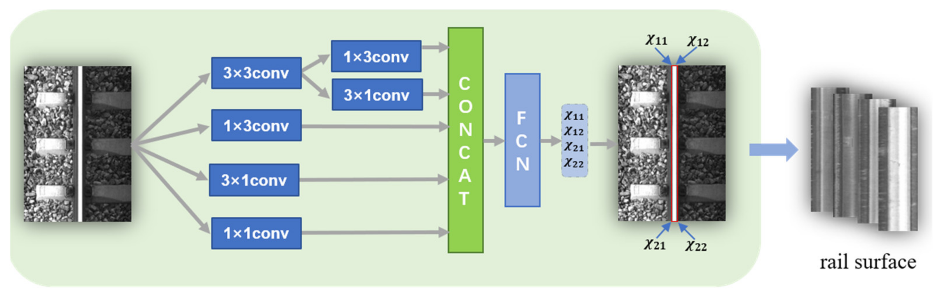
2.1.1. Rail Surface Detection

The purpose of rail surface detection is to locate the pixels of the rail surface area from the original rail inspection images (including rail surface, fasteners, rail sleepers, etc.,) and to extract them for the next stage of defect detection. In order to accurately locate the rail surface from the original rail inspection image, we proposed a lightweight RC-Net based on inception blocks [28], considering the characteristics of the rail inspection image and the task requirements. As shown in Figure 2 stage 1: rail surface detection, the input of RC-Net is the inspection image, and the output is the transverse coordinates of the four vertex pixels (x₁₁, x₁₂, x₂₁, x₂₂) of the rail surface.

2.1.2. Defect Detection

The detection and extraction of the rail surface from the original rail inspection image largely reduced the influence of the remaining background elements such as fasteners and ballast in the detection of defects. To perform defect detection, our basic idea is to reconstruct the defected rail surface image into a normal rail surface image without defects by means of an auto-encoder, and then segment the defects by the residual map between the defected rail surface image and the reconstructed image. To improve the quality of the reconstructed image and the accuracy of the defect segmentation, we add random pseudo-defects as self-supervised signals to the introspective variational auto-encoder in the training process. Thus we proposed the DR-VAE for the background reconstruction, so that the segmentation and anomaly detection of rail surface defects could be performed by the residual map and structured similarity between the input image and the reconstructed image. As shown in Figure 2 stage 2: rail defect detection, in the training phase, an X_nr (normal rail surface image) was firstly masked with random defects by Bézier–Gaussian random pseudo-defects, and then X_dr (masked image) was fed into the variational autoencoder for image reconstruction. Then, following with masking both X_rr (reconstructed image) and X_fr (image derived from the decoder independently sampled and reconstructed) with random defects and feeding them into the variational autoencoder, an introspective self-supervised training process was performed. In the inference stage, X_rdr (real rail surface image) was fed into the trained variational autoencoder for background reconstruction, and then X_ri (residual image), between X_rrr (reconstructed image) and X_rdr, was binarized through the threshold T₁ to obtain X_ti (segmented image). The anomaly scores of X_rdr and X_rrr were also calculated, and the final anomaly detection result was obtained through the threshold T₂.

2.2. Rail Surface Detection

Based on the previous analysis, this paper proposed a simple and effective RC-Net for detection and extraction of the rail surface image from the rail inspection image. As shown in Figure 3, the input of RC-Net is the inspection image, and the output is the transverse coordinates of the four vertex pixels (x₁₁, x₁₂, x₂₁, x₂₂) of the rail surface. In order to minimize the capacity and improve the accuracy of model, we have streamlined the RC-Net to the maximum extent possible. The backbone consists of only an inception module [28] and a fully connected layer. The inception module consists of the 3 × 3, 1 × 1, 1 × 3 and 3 × 1 convolution layers to extract the edge pixels of the rail surface accurately. The 3 × 3 and 1 × 1 convolution kernels facilitate the extraction of local information of the rail edges compared to the large size convolution kernels, and the combination of the 1 × 3 and 3 × 1 convolution layers provides more diverse feature descriptions while reducing the computational effort, compared to the 3 × 3 convolution layer. Ultimately, for subsequent stages of model training and inference, we extracted the rail surface images based on the network output of the rail surface coordinates.

In fact, the data complexity of the rail inspection images is much lower than the initial task data complexity of detection models such as YOLOV4 [29] or Faster-RCNN [30]. Actually, the model only needs to regress four parameters to locate the rail surface area without redundant structures such as RPN and category output, since there is only one class of targets and little variation in target scales. It is worth noting that four regression parameters are necessary to accommodate the extraction of non-rectangular rail surface regions, where x₁₁ is the upper left edge transverse coordinates of the rail surface, x₁₂ refers to the upper right one, and so on.

2.3. Defect Detection

As we previously obtained rail surface images, this section details the rail surface defect detection model DR-VAE, including the training and the inference architecture, of which the training architecture is shown in Figure 4. Firstly, a Bézier–Gaussian random pseudo-defect was generated with an arbitrary shape and a random grayscale. Secondly, the D-RM module was used to add randomly located pseudo-defects to X_nr to generate self-supervised data. At the same time, the DR-VAE also performed an introspective adversarial training process. The details of each part are described in detail below.

2.3.1. Defect Random Mask

To perform self-supervised training [31], we combined Bézier curves with Gaussian random noise to generate pseudo-defect blocks of an arbitrary shape and size [32], and masked the rail surface with it to generate the rail surface containing pseudo-defects as a self-supervised signal. We first generated contours of pseudo-defects with arbitrary shapes using Bézier curves. For any n normalized points in the plane {P_i|i = 1, 2, …, n}, we used a parametric equation B(t), t ∈ 5(0,1) to define the n − 1 order Bézier curve between the first and last two points, as shown in Equation (1).

$$B\left(t\right)={\displaystyle {\sum }_{j=0}^n{t}^j{\displaystyle {\prod }_{s=0}^{j-1}(n-s){\displaystyle {\sum }_{i=0}^j\frac{{\left(-1\right)}^{i+j}{P}_i}{i!\left(j-i\right)!}}}}$$

(1)

The closed curve randomly generated by the Bézier curve was filled with a sequence of randomly decaying Gaussian noise pixels, which makes the final generated random pseudo-defects to be similar to the real rail surface defects. Since directly using Gaussian random noise pixels, to fill the contour generated by the Bézier curve, could not generate random defects close to the real distribution, we introduced a random attenuation factor ζ to the Gaussian random noise, which randomly limits the sampling range of the Gaussian noise to produce a random defective pixel grayscale sequence G(k), as in Equation (2).

$$G\left(k\right)=255\zeta z_k^2$$

(2)

where z_k~N(0,1) is a sampled value from the standard Gaussian distribution, k is the number of pixel points contained in the random contour, ζ ∈ (0,1) is the attenuation factor. The average grayscale value of the generated pixels will be smaller with a smaller value of ζ, and a darker defect will be obtained as a whole. It was then filled into contour to generate a Bézier–Gaussian random pseudo-defect close to the true distribution, as shown in Figure 5.

To obtain the final rail surface containing random pseudo-defects, we used a random factor to generate a random mask location based on the scale of the outer square of the random pseudo-defect. The initial position of the random mask is shown in Equations (3) and (4).

$$P\left(x_m\right)=\left(W-d\right)u_m$$

(3)

$$P\left(y_m\right)=\left(H-d\right)u_m$$

(4)

where m is a mask number, P(x_m) and P(y_m) denote the coordinates of the initial position of the random mask with number m. W and H denote the width and height of the rail surface image. The length of the outer square of the pseudo-defect block is represented by d, and u_m~U(0,1) is a random factor obtained from uniform distribution. The partial rail surface image masked by random pseudo-defect with m = 1 is shown in Figure 6.

2.3.2. Training Framework

The goal of the DR-VAE training framework is to detect defects on the rail surface image based on reconstruction error. The reconstruction error of the defective regions will be larger than that of the normal regions when it exists in the input image. In order to improve the clarity of the reconstructed image while avoiding model redundancy with additional adversarial structure, DR-VAE uses the decoder as a discriminator at the same time to achieve adversarial training. Meanwhile, the encoder and decoder in different parts of the training framework, use the same network structure and share the weight parameters. The corresponding block module consists of multiple residual blocks [28], which can capture the key information in the case of a simple structure. As shown in

Table 1. Model parameters of encoder and decoder.

Encoder	Parameters	Output	Decoders	Parameters	Output
Input	-	64 × 64 × 1	L-vector	-	8 × 1 × 1
Conv	5 × 5, 8	64 × 64 × 8	FC-16	16	16 × 1 × 1
Avg pool	-	32 × 32 × 8	FC-1024	1024	1024 × 1 × 1
Res-block	1 × 1, 16 3 × 2, 16 3 × 3, 16		Reshape	-	4 × 4 × 64
		32 × 32 × 16	Res-block	3 × 3, 64 3 × 3, 64	4 × 4 × 64
Avg pool	-	16 × 16 × 16	Up-sample	-	8 × 8 × 64
Res-block	1 × 1, 32 3 × 3, 32 3 × 3, 32		Res-block	1 × 1, 32 3 × 3, 32 3 × 3, 32
		16 × 16 × 32			8 × 8 × 32
Avg pool	-	8 × 8 × 32	Up-sample	-	16 × 16 × 32
Res-block	1 × 1, 64 3 × 3, 64 3 × 3, 64		Res-block	3 × 3, 16 3 × 3, 16	16 × 16 × 16
		8 × 8 × 64
			Up-sample	-	32 × 32 × 16
Avg pool	-	4 × 4 × 64	Res-block	3 × 3, 8 3 × 3, 8	32 × 32 × 8
Reshape	-	1024 × 1 × 1
FC-16	16	16 × 1 × 1	Up-sample	-	64 × 64 × 8
Split	-	8,8	Conv	5 × 5, 1	64 × 64 × 1

, the encoder consists of stacked residual blocks and averaged pooling layers with increasing channel dimensionality. The input is the rail surface image and the output is the eight-dimensional Gaussian distribution parameters (µ,σ). The decoder consists of a stacked residual block and up-sampling layers with decreasing channel dimension. The input is the sampled values from the aforementioned Gaussian distribution, and the output is the reconstructed rail surface images.

The loss function of our proposed DR-VAE model in the training process includes KL divergence loss and pixel loss. KL divergence is used to measure how similar the latent space distribution, obtained by the encoder, is to the standard Gaussian distribution [33]; and reducing the KL divergence loss can make the pixel grayscale distribution of the reconstructed image more uniform and consistent. The relevant loss functions involved in this paper include the original KL divergence and the introspective KL divergence, as in Equations (5) and (6).

$$KL=\frac{1}{2}{\displaystyle \sum }_{i=1}^N{\displaystyle \sum }_{j=1}^M\left(1+\log \left({\sigma }_{ij}^2\right)-{\mu }_{ij}^2+{\sigma }_{ij}^2\right)$$

(5)

$$K{L}_{intro}=\frac{1}{2}{\displaystyle \sum }_{i=1}^N{\displaystyle \sum }_{j=1}^M\left(1+\log \left({\sigma }_s{}_{ij}^2\right)-{\mu }_s{}_{ij}^2+{\sigma }_s{}_{ij}^2\right)$$

(6)

where μ and σ are latent space distribution parameters that, estimated by the encoder, N, is the minimum batch number, M represents the dimensionality of the latent vectors (z and z_s) sampled from N(μ, σ), and s denotes that the KL_intro contains the KL loss of two different branches in the introspective reconstruction part.

Since the actual running rail surface background is very complex and the difference between abnormal features and normal background features is small, which is often polluted by non-defective features such as dirt and rust, we introduced the structured similarity metric (SSIM) [27] instead of the mean square error as the pixel loss function, including the L_SSIM and the introspective $L_{SSI{M}_{intro}}$, as in Equations (7) and (8):

$$L_{SSIM}=\frac{1}{2}{\displaystyle \sum _{i=1}^{N}SSIM\left(x_{r{r}_i},x_{n{r}_i}\right)}$$

(7)

$$L_{SSI{M}_{intro}}=\frac{1}{2}{\displaystyle \sum }_{i=1}^{N}SSIM\left(x_{frr{s}_i},x_{n{r}_i}\right)$$

(8)

where N denotes the minimum batch number, x_nr is the normal rail image, x_rr is the reconstructed rail image, and x_frrs is the introspective reconstructed rail image; s contains two different branches in the introspective reconstruction part.

The total loss function of the encoder is shown in Equation (9).

$$L\left({\varphi }_E\right)=\frac{1}{d}({\alpha }_{kl}KL+\beta L_{SSIM})-\frac{1}{2}exp\left[-\frac{2}{d}{\displaystyle \sum }_{s=u,v}({\alpha }_{neg}K{L}_{intro}+\beta L_{SSI{M}_{intro}})\right]$$

(9)

The total loss of the decoder is shown in Equation (10).

$$L\left({\theta }_D\right)=\frac{1}{d}\left[\beta L_{SSIM}+{\displaystyle \sum }_{s=u,v}\left({\alpha }_{neg}K{L}_{intro}+\gamma \beta L_{SSI{M}_{intro}}\right)\right]$$

(10)

where d is the input image dimension, α_kl, β, α_neg, γ are hyperparameters, indicating the proportion of each type of loss in the total loss.

Our proposed self-supervised training framework is divided into real rail reconstruction and introspective reconstruction, for which both parts introduce Bézier–Gaussian random pseudo-defects as self-supervised signals. To train the model, we firstly initialized the model hyperparameters and weight parameters; secondly we fixed the decoder weight parameters θ_D and trained the encoder weight parameters ϕ_E; thirdly we fixed the encoder weight parameters ϕ_E and trained the decoder weight parameters θ_D, and finally we iterated the above process until the model converged. The pseudocode is shown in Algorithm 1.

Algorithm 1 DR-VAE training pseudocode

Requireαkl, β, αneg, γ, ϕE, θD

while not converged do.

Xnr ← Get the normal rail surface data for a batch

Xdr ← D-RM(Xnr) generates pseudo-random defective rail surface data

μ,σ ← E(Xdr); z←μ + εσ;zf ← sampled from N(0,1)

Update Encoder E (ϕE).:

Xrr ← D(z); Xfr ← D(zf); Xdrr ←D-RM(Xrr); Xdfr ← D-RM(Xfr)

μs, σs ← E(Xddr, Xdfr); zs ← μs +εσs; Xfrrs ← D(zs)

KL← μ,σ; KLintro ←μs, σs

L ← XSSIMrr, Xnr; LSSIM(intro) ← Xffrs, Xn

L(ϕE) ← (αklKL + βLSSIM)/d − 0.5exp(−2(αnegKLintro + βLSSIM(intro)))/d

ϕE← ϕE − η∇L(ϕE)

end update

Update decoder D (θD):

Xrr ← D(z); Xfr ← D(zf); Xdrr ← D-RM(Xrr); Xdfr ← D-RM(Xfr)

μs, σs ← E(Xddr, Xdfr); zs ← μs + εσs; Xfrrs ← D(zs)

KLintro ← μs, σs; LSSIM ← Xrr, Xnr; LSSIM(intro) ← Xffrs, Xn

L(θD) ← βLSSIM/d + (αneg KLintro + γβLSSIM(intro))/d

θD← θD − η∇L(θD)

end update

end while

2.3.3. Model Inference

The goal of the DR-VAE inference model is to detect defects in the rail surface image based on the reconstruction error. Due to the presence of the sampling process from the standard Gaussian distribution, the background reconstruction process adds a random factor, which leads to the unstable quality of the reconstructed image. However, the consistency of the grayscale distribution of the reconstructed image is also guaranteed by the sampling process from the standard normal distribution. Therefore, in the inference, we introduced a distribution capacity attenuation factor δ to limit the range of sampling values z based on the VAE re-parameterization technique [34], so as to improve the stability of the reconstructed image and ensure the consistency of the grayscale distribution of the image. As shown in Equation (11).

$$z=\mu +\delta \epsilon \sigma$$

(11)

where μ and σ are latent space distribution parameters that are estimated by the encoder, ε~N(0, 1) is a sampled value from the standard Gaussian distribution, and δ ∈ (0, 1) is a hyperparameter.

To achieve anomaly detection and defect segmentation of rail surface defects, we first calculated the anomaly score by the structured similarity between the input image and the reconstructed image [27], and this algorithm measures the similarity of the image by brightness, contrast and structure, as shown in Equation (12).

$$SSIM(x_i,x_r)=\frac{(2{\mu }_i{\mu }_r+a_1)(2{\sigma }_{ir}+a_2)}{({\mu }_i^2+{\mu }_r^2+a_1)({\sigma }_i^2+{\sigma }_r^2+a_2)}$$

(12)

where x_i is the input image and x_r is the reconstructed image. μ_i and μ_r, σ_i and σ_r, and σ_ir are the mean, standard deviation and covariance of x_i and x_r, respectively.a₁ and a₂ are constants to ensure computational stability, and a₁ = 0.01 and a₂ = 0.03, as usual. The anomaly fraction between x_i and x_r is determined by thresholding T₂. Finally, we segmented the residual map corresponding to the rail surface image containing defects by T₁ to achieve the detection of rail surface defects.

3. Results and Analysis

In order to evaluate the performance of the proposed rail surface defect detection system, we performed experiments on the private image dataset collected by the GTC-80J rail inspection vehicle in Gansu, China, as is shown in Figure 7. The dataset contains about 17,000 rail inspection images with a resolution of 1500 × 2180 pixels. The experimental environment is as follows: Ubuntu 16.04, Python 3.7, Keras-2.2.4-TensorFlow-gpu-2.6, Intel(R) Core(TM) i7-7700HQ CPU with 2.80 GHz and NVIDIA Quadro P2000 GPU with 5 GB RAM.

3.1. Rail Surface Detection

In this section, we evaluated the performance of the RC-NET. The original rail inspection image dataset is randomly divided into two parts: 11,000 images for training and 6000 images for testing. To investigate the effect of the convolution scale and the fully connected layer capacity on the detection accuracy, we compared the model performance with a different convolution scale n and fully connected layer capacity m by PR curves. P denotes the precision, which is defined by the proportion of true defect pixels among pixels predicted to be defective. R denotes the recall rate, which is defined by the proportion of correctly predicted defect pixels among the total defect pixels. The AUC denotes the area of the region bounded by the curve and the coordinate axis, and its ideal value is 1. As shown in Figure 8.

It can be found that the model has the best overall performance when the AUC = 0.931 for the PR curve with a convolution scale n = 3 and fully connected layer capacity of m = 16. The discussion and analysis are as follows: (i) A large convolution scale n leads to a decrease in the model’s ability to recognize fine-grained features, which are important for the model to recognize the edges of the railroad surface. However, a small convolution scale n leads to a smaller perceptual field, which makes the model less able to extract abstract features. (ii) If the capacity m of the fully connected layer is too small, the model will underfit the training data, making it difficult for the model to converge in training. However, too large a capacity will lead to very severe overfitting of the model during training, which will make the model less accurate for testing.

To further validate the model performance, we also compared the RC-Net with several deep learning object detection methods, including YOLOv4 [29], Faster R-CNN [30], and SSD [34]. For a fair comparison, all of these algorithms used the same training dataset and annotation. After training, the IOU threshold was set to 0.7, and the performance of each object detection algorithm was evaluated using precision, recall and F1 score metrics. The results of the rail surface detection are shown in

Table 2. Comparison of different rail surface detection models.

Models	Precision	Recall	F1 Score
Faster R-CNN	0.991	0.979	0.985
YOLOv4	0.979	0.978	0.979
SSD	0.985	0.975	0.980
RC-Net	0.992	0.985	0.988

. It can be found that the deep learning object detection method performed well in rail surface detection. Compared with the other listed methods, RC-NET outperforms on rail surface detection with an accuracy of 0.992, a recall of 0.985 and an F1 score of 0.988, based on a greatly simplified model structure.

3.2. Rail Surface Defect Detection

In this section, we evaluated the performance of the proposed defect detector DR-VAE. In our experiments, we selected 10,000 rail inspection images with normal rail surfaces and extracted rail regions using RC-Net. Then we trained DR-VAE with a momentum of 0.8, weight decay of 3 × 10⁻⁴ and batch size of 32, for a total of 300 epochs. The learning rate was set to 0.001 and a decay of 0.5 times every 60 epochs. To test the performance of DR-VAE, we mixed the remaining 6000 normal railroad surface images with 146 images containing defects and disordered them. The capacity attenuation factor δ and Bézier–Gaussian random pseudo-defects are the main factors that affect the performance of the model To investigate the actual effect of them, we compared the model performance with different pseudo-defect scales d and the capacity attenuation factor δ using P-R curves. This is shown in Figure 9.

The experiments showed that the model has the best overall performance with the AUC of 0.922 at d of 15 and δ of 0.2. The reason is that, if pseudo-random defects are too large, this will lead to large differences between the distribution of the self-supervised signal and the original defective data, thus leading to a limitation of the effectiveness of the self-supervised training. Meanwhile, too small a distribution capacity attenuation factor will lead to over concentrated distribution of the reconstructed data, thus making it very different from the real track surface; while too large a distribution capacity attenuation factor will lead to much randomness in the distribution of the reconstructed data, thus leading to over generalization of the model, which further leads to a decrease in the reconstruction accuracy of the reconstructed data of non-defective pixels.

To evaluate the ability of DR-VAE to detect the rail surface defects, we conducted comparison experiments using PR curves and ROC curves (receiver operating characteristic curves). ROC curves do not vary with the classification distribution and are a widely used evaluation for classifiers with unbalanced binary prediction problems because they are not biased towards majority or minority classes. Contrast algorithms included GANomaly [21], AnoGAN [23], MemAE [25], and Soft-IntroVAE [27]. Figure 10 show the ROC and PR curves on the rail surface dataset to see that the proposed DR-VAE has an AUC = 0.933 for the PR curve and an AUC = 0.958 for the ROC curve, which has a significant advantage over other leading methods. The reason is that our proposed model greatly improves the ability on the removal of defects while retaining enough critical information of normal images through self-supervised learning. Meanwhile, the sharpness of the reconstructed rail surface images is also improved through introspective adversarial training.

For a more comprehensive and objective evaluation, we also introduced accuracy rate (ACC) F1 score and Matthews correlation coefficient (MCC, range [−1, 1]) as auxiliary evaluation metrics. Using the value synthesis confusion matrix, MCC measures the correlation between the true value and inference. The results of the defect detection evaluation on the rail surface dataset are listed in

Table 3. Comparison of different rail surface defect detection methods.

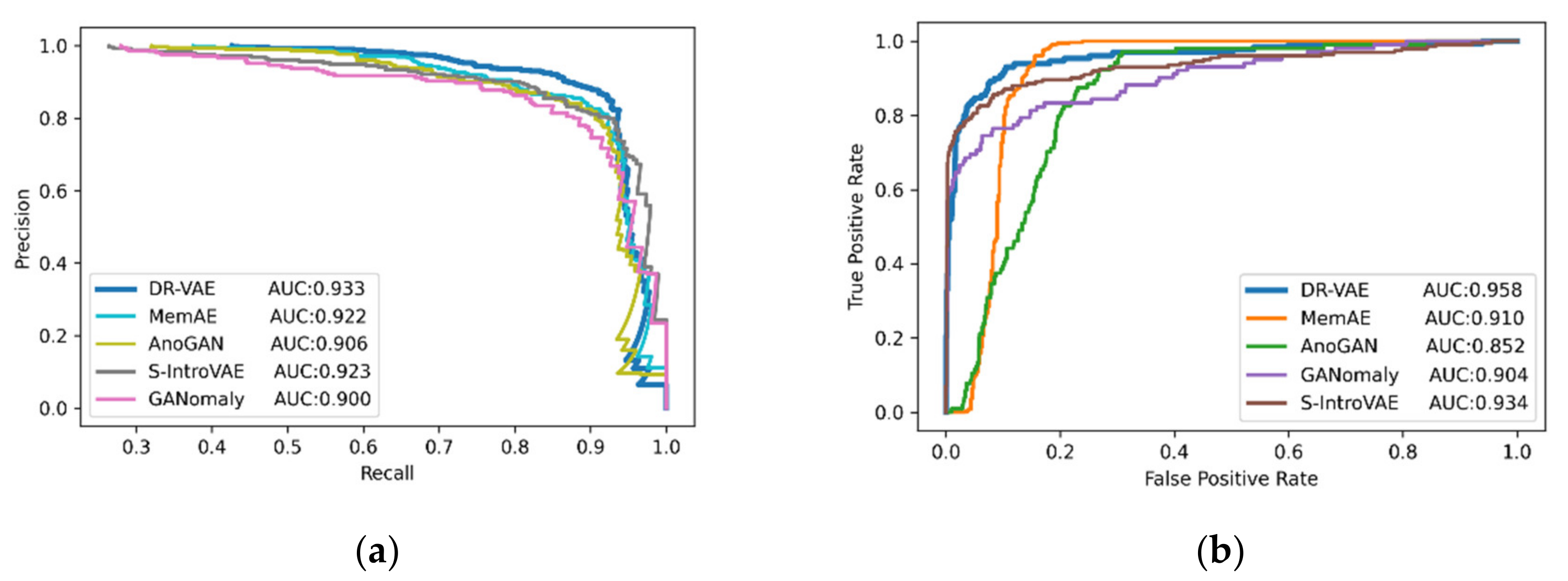
Models	ACC	Precision	Recall	MCC	AUC	F1
MemAE	0.69	0.91	0.47	0.58	0.922	0.74
Soft-IntroVAE	0.68	0.93	0.46	0.57	0.923	0.78
GANomaly	0.68	0.92	0.46	0.57	0.900	0.73
AnoGAN	0.52	0.86	0.31	0.49	0.906	0.50
DR-VAE	0.71	0.95	0.48	0.59	0.933	0.81

and show the effectiveness of our approach. The best results on accuracy and recall indicate that normal and abnormal samples can be accurately identified. In addition, two classification metrics (MCC, F1) also prove the superiority of our method. The representative defect segmentation results are shown in Figure 11.

Compared with supervised deep learning methods, the proposed method in this paper overcomes the disadvantage of the requirement for a large number of defect-containing samples. The encoding vector of DR-VAE is derived from a random sample (Gaussian distribution) with uniform structure in the latent space; with this randomness, the decoder still has to reconstruct the defect-free background in the training phase, which makes its defect suppression stronger. The incorporated Bézier–Gaussian pseudo-defects provided the model with a self-supervised signal and therefore it has an advantage for defect removal and background reconstruction. At the same time, the random error is greatly reduced by introducing a distribution capacity attenuation factor in the inference stage, which maximizes the sharpness of the reconstructed image, while avoiding a wide range of grayscale panning.

4. Conclusions

The two-stage structure proposed in this paper combined supervised and self-supervised learning methods to complete the training of the model, and automatically locate the rail surface and detect defects from the rail inspection images under the condition of unbalanced samples. Compared to supervised learning methods, our proposed method requires only easily accessible normal samples during training, without directly addressing the problem of the imbalance of samples due to insufficient defective samples. Also the proposed method improves the defect removal ability and background reconstruction quality of the model compared to other unsupervised methods, due to the integration of the introspective training framework with random pseudo-defects as self-supervised signals, which leads to the improvement of the defect detection accuracy of the model. We analyzed the effects of the main parameters of RC-Net and DR-VAE on the model performance and compared the model with related alternative methods. The main parameter experiments showed that the rail surface detection model RC-Net has the best overall performance with the AUC = 0.931 of the PR curve at the convolution scale n = 3 and the fully connected layer capacity m = 16. The defect detection model DR-VAE had the best overall performance with AUC = 0.922 at random pseudo-defect scale d = 15 and distribution capacity attenuation factor δ = 0.2. Comparative experiments related to RC-Net showed that it can ensure the accuracy of rail surface region detection in practice with a simplified network structure. Compared with other methods, it also indicated that DR-VAE performs well with the AUC, precision, recall and other evaluation metrics. The experimental results showed that RC-Net and DR-VAE outperform other testing methods and can effectively detect railroad surface defects. Therefore, the proposed method can be implemented in a railroad surface inspection system for detecting railroad surface defects. However, the two-stage process made the training process tedious, and subsequent research should design an end-to-end defect detection framework to simplify the training process. Meanwhile, in the application research of deep learning algorithms, the simplification of the network structure and the regulation of hyperparameters often appear to be crucial. In this paper, we have completed a part of the comparative research and achieved good results. Therefore, how to minimize the network and make it more lightweight while ensuring the model accuracy and inference rate is still a direction worthy of research.

References

- Cao, X.; Xie, W.; Ahmed, S.M.; Li, C.R. Defect Detection Method for Rail Surface Based on Line-Structured Light. Measurement 2020, 159, 107771. [Google Scholar] [CrossRef]
- Haomin, Y.; Li, Q.; Tan, Y.; Gan, J.; Wang, J.; Geng, Y.; Jia, L. A Coarse-to-Fine Model for Rail Surface Defect Detection. IEEE Trans. Instrum. Meas. 2019, 68, 656–666. [Google Scholar] [CrossRef]
- Gan, J.; Li, Q.; Wang, J.; Yu, H. A Hierarchical Extractor-Based Visual Rail Surface Inspection System. IEEE Sens. J. 2017, 17, 7935–7944. [Google Scholar] [CrossRef]
- Ni, X.; Ma, Z.; Liu, J.; Shi, B.; Liu, H. Attention Network for Rail Surface Defect Detection via Consistency of Intersection-over-Union(IoU)-Guided Center-Point Estimation. IEEE Trans. Ind. Inform. 2022, 18, 1694–1705. [Google Scholar] [CrossRef]
- Hajizadeh, S.; Núñez, A.; Tax, D.M.J. Semi-Supervised Rail Defect Detection from Imbalanced Image Data. IFAC-Pap. 2016, 49, 78–83. [Google Scholar] [CrossRef]
- Yaman, O.; Karakose, M.; Akin, E. A Vision Based Diagnosis Approach for Multi Rail Surface Faults Using Fuzzy Classificiation in Railways. In Proceedings of the 2017 International Conference on Computer Science and Engineering (UBMK), Antalya, Turkey, 5–8 October 2017; pp. 713–718. [Google Scholar]
- Yuan, H.; Chen, H.; Liu, S.; Lin, J.; Luo, X. A Deep Convolutional Neural Network for Detection of Rail Surface Defect. In Proceedings of the 2019 IEEE Vehicle Power and Propulsion Conference (VPPC), Hanoi, Vietnam, 14–17 October 2019; pp. 1–4. [Google Scholar]
- Jin, X.; Wang, Y.; Zhang, H.; Zhong, H.; Liu, L.; Wu, Q.M.J.; Yang, Y. DM-RIS: Deep Multimodel Rail Inspection System with Improved MRF-GMM and CNN. IEEE Trans. Instrum. Meas. 2020, 69, 1051–1065. [Google Scholar] [CrossRef]
- Sabokrou, M.; Khalooei, M.; Fathy, M.; Adeli, E. Adversarially Learned One-Class Classifier for Novelty Detection. In Proceedings of the 2018 IEEE/CVF Conference on Computer Vision and Pattern Recognition, Salt Lake City, UT, USA, 18–23 June 2018; pp. 3379–3388. [Google Scholar]
- Nawaratne, R.; Alahakoon, D.; De Silva, D.; Yu, X. Spatiotemporal Anomaly Detection Using Deep Learning for Real-Time Video Surveillance. IEEE Trans. Ind. Inform. 2020, 16, 393–402. [Google Scholar] [CrossRef]
- He, Y.; Peng, Y.; Wang, S.; Liu, D. ADMOST: UAV Flight Data Anomaly Detection and Mitigation via Online Subspace Tracking. IEEE Trans. Instrum. Meas. 2019, 68, 1035–1044. [Google Scholar] [CrossRef]
- Castellani, A.; Schmitt, S.; Squartini, S. Real-World Anomaly Detection by Using Digital Twin Systems and Weakly Supervised Learning. IEEE Trans. Ind. Inform. 2021, 17, 4733–4742. [Google Scholar] [CrossRef]
- Luo, Q.; Fang, X.; Liu, L.; Yang, C.; Sun, Y. Automated Visual Defect Detection for Flat Steel Surface: A Survey. IEEE Trans. Instrum. Meas. 2020, 69, 626–644. [Google Scholar] [CrossRef] [Green Version]
- Xiong, L.; Póczos, B.; Schneider, J. Group Anomaly Detection Using Flexible Genre Models. In Advances in Neural Information Processing Systems; Shawe-Taylor, J., Zemel, R., Bartlett, P., Pereira, F., Weinberger, K.Q., Eds.; Curran Associates, Inc.: Red Hook, NY, USA, 2011; Volume 24. [Google Scholar]
- Zhuang, B.; Shen, C.; Tan, M.; Liu, L.; Reid, I. Structured Binary Neural Networks for Accurate Image Classification and Semantic Segmentation. In Proceedings of the 2019 IEEE/CVF Conference on Computer Vision and Pattern Recognition (CVPR), Long Beach, CA, USA, 15–20 June 2019; pp. 413–422. [Google Scholar]
- Zong, B.; Song, Q.; Min, M.R.; Cheng, W.; Lumezanu, C.; Cho, D.; Chen, H. Deep Autoencoding Gaussian Mixture Model for Unsupervised Anomaly Detection. In Proceedings of the International Conference on Learning Representations, Vancouver, BC, Canada, 15 February 2018; pp. 1–19. [Google Scholar]
- Hasan, M.; Choi, J.; Neumann, J.; Roy-Chowdhury, A.K.; Davis, L.S. Learning Temporal Regularity in Video Sequences. In Proceedings of the 2016 IEEE Conference on Computer Vision and Pattern Recognition (CVPR), Las Vegas, NV, USA, 30 June 2016; pp. 733–742. [Google Scholar]
- Zhao, Y.; Deng, B.; Shen, C.; Liu, Y.; Lu, H.; Hua, X.-S. Spatio-Temporal AutoEncoder for Video Anomaly Detection. In Proceedings of the 25th ACM International Conference on Multimedia, New York, NY, USA, 23–27 October 2017; pp. 1933–1941. [Google Scholar]
- Akcay, S.; Atapour-Abarghouei, A.; Breckon, T.P. GANomaly: Semi-Supervised Anomaly Detection via Adversarial Training. In Proceedings of the Computer Vision–ACCV 2018, Perth, Australia, 2–6 December 2018; Jawahar, C.V., Li, H., Mori, G., Schindler, K., Eds.; Springer: Cham, Switzerland, 2019; pp. 622–637. [Google Scholar]
- Medel, J.R.; Savakis, A. Anomaly Detection in Video Using Predictive Convolutional Long Short-Term Memory Networks. arXiv 2016, arXiv:1612.00390. [Google Scholar]
- Perera, P.; Nallapati, R.; Xiang, B. OCGAN: One-Class Novelty Detection Using GANs with Constrained Latent Representations. In Proceedings of the 2019 IEEE/CVF Conference on Computer Vision and Pattern Recognition (CVPR), Long Beach, CA, USA, 15–20 June 2019; pp. 2893–2901. [Google Scholar]
- Schlegl, T.; Seeböck, P.; Waldstein, S.M.; Schmidt-Erfurth, U.; Langs, G. Unsupervised Anomaly Detection with Generative Adversarial Networks to Guide Marker Discovery. In Proceedings of the Information Processing in Medical Imaging, Boone, NC, USA, 25–30 June 2017; Niethammer, M., Styner, M., Aylward, S., Zhu, H., Oguz, I., Yap, P.-T., Shen, D., Eds.; Springer: Cham, Switzerland, 2017; pp. 146–157. [Google Scholar]
- Zenati, H.; Romain, M.; Foo, C.-S.; Lecouat, B.; Chandrasekhar, V. Adversarially Learned Anomaly Detection. In Proceedings of the 2018 IEEE International Conference on Data Mining (ICDM), Singapore, 17–20 November 2018; pp. 727–736. [Google Scholar]
- Gong, D.; Liu, L.; Le, V.; Saha, B.; Mansour, M.R.; Venkatesh, S.; Van Den Hengel, A. Memorizing Normality to Detect Anomaly: Memory-Augmented Deep Autoencoder for Unsupervised Anomaly Detection. In Proceedings of the 2019 IEEE/CVF International Conference on Computer Vision (ICCV), Seoul, Korea, 27 October–2 November 2019; pp. 1705–1714. [Google Scholar]
- Ye, F.; Huang, C.; Cao, J.; Li, M.; Zhang, Y.; Lu, C. Attribute Restoration Framework for Anomaly Detection. IEEE Trans. Multimed. 2022, 24, 116–127. [Google Scholar] [CrossRef]
- Daniel, T.; Tamar, A. Soft-IntroVAE: Analyzing and Improving the Introspective Variational Autoencoder. In Proceedings of the 2021 IEEE/CVF Conference on Computer Vision and Pattern Recognition (CVPR), Nashville, TN, USA, 19 June 2021; pp. 4389–4398. [Google Scholar]
- Bergmann, P.; Löwe, S.; Fauser, M.; Sattlegger, D.; Steger, C. Improving Unsupervised Defect Segmentation by Applying Structural Similarity to Autoencoders. arXiv 2018, arXiv:1807.02011. [Google Scholar]
- Szegedy, C.; Ioffe, S.; Vanhoucke, V.; Alemi, A. Inception-v4, Inception-ResNet and the Impact of Residual Connections on Learning. arXiv 2016, arXiv:1602.07261. [Google Scholar]
- Bochkovskiy, A.; Wang, C.-Y.; Liao, H.-Y.M. YOLOv4: Optimal Speed and Accuracy of Object Detection. arXiv 2020, arXiv:2004.10934. [Google Scholar]
- Ren, S.; He, K.; Girshick, R.; Sun, J. Faster R-CNN: Towards Real-Time Object Detection with Region Proposal Networks. In Proceedings of the 28th International Conference on Neural Information Processing Systems, Montreal, QC, Canada, 7–12 December 2015; MIT Press: Cambridge, MA, USA, 2015; Volume 1, pp. 91–99. [Google Scholar]
- He, K.; Chen, X.; Xie, S.; Li, Y.; Dollár, P.; Girshick, R. Masked Autoencoders Are Scalable Vision Learners. arXiv 2021, arXiv:2111.06377. [Google Scholar]
- Viquerat, J.; Hachem, E. A Supervised Neural Network for Drag Prediction of Arbitrary 2D Shapes in Laminar Flows at Low Reynolds Number. Comput. Fluids 2020, 210, 104645. [Google Scholar] [CrossRef]
- Kingma, D.P.; Welling, M. Auto-Encoding Variational Bayes. arXiv 2014, arXiv:1312.6114. [Google Scholar]
- Liu, W.; Anguelov, D.; Erhan, D.; Szegedy, C.; Reed, S.; Fu, C.-Y.; Berg, A.C. SSD: Single Shot MultiBox Detector. In Proceedings of the Computer Vision–ECCV 2016, Amsterdam, The Netherlands, 11–14 October 2016; Leibe, B., Matas, J., Sebe, N., Welling, M., Eds.; Springer: Cham, Switzerland, 2016; pp. 21–37. [Google Scholar]