Transient Stability Analysis and Post-Fault Restart Strategy for Current-Limited Grid-Forming Converter

Abstract

Grid-forming converters are attracting attention for their significant advantages in terms of stability in a weak grid and simulated inertia. However, while they offer great flexibility due to the use of power semiconductors, they are also affected by their low current-carrying capacity. This means that during a fault, instead of the usual voltage control, a current limiting control is active, which changes the dynamic performance of the converter and influences transient stability. This manuscript focuses on the dynamic performance of grid-forming converters during the restart phase at the post-fault period, and proposes an initial phase threshold to prevent the converter from going into current saturation. Based on this, the manuscript proposes several restart strategies during the post-fault period, by using some fast resynchronization methods in order to meet the requirements of the converter’s stable operation and fast active power restoration. Finally, the above findings and the proposed strategies are validated by a joint control hardware-in-the-loop system.

1. Introduction

As the 2030 climate and energy framework [1] targets for renewable energy are gradually being met, investment in renewable energy is also on the rise. The combination of renewable energy sources and grid-connected converters brings more flexibility to the power system [2]. However, grid-connected converters also pose problems for a power system such as stability in a weak grid [3,4], a lack of inertia [5], and even causing some accidents [6,7] in the last few years. In order to compensate for the shortcomings of using grid-connected converters, the grid-forming concept was proposed [8,9,10,11].

Grid-forming converters differ from conventional grid-connected converters in their control method rather than in their hardware topology. Firstly, the control method uses an active power-frequency (P-f) loop to control its output active power, so that it automatically simulates inertia to enhance the frequency stability of the grid [12]. Secondly, it uses a controlled voltage source mode to control its output voltage, so the robustness in weak grids is also enhanced in the sense of its small-signal stability [13].

However, the transient characteristic of grid-forming converters during faults is limited by the current-carrying capacity of the power semiconductor components [14]. When the grid voltage drops, grid-forming converters cannot perform their original dynamic performance due to the current saturation [15]. Optimized grid-forming strategies have been proposed for fault ride through capability [16,17,18,19,20,21,22]. However, more experience has been gained with phase-locked loop (PLL)-based techniques to fulfill the control requirements of negative sequence currents in grid codes [23], particularly for reactive current injection in positive and negative sequences [24,25]. Therefore, mostly, grid-forming converters currently activate a backup PLL during the Low-Voltage Ride Through (LVRT), thus temporarily turning into a grid following-like converter [8,26] so as to meet the requirement for the reactive current injection in negative sequences. After the fault clearing, the converter then reactivates its P-f loop to restore its grid-forming characteristics.

In the study of LVRT strategies for grid-forming converters, most of the literature has focused on the stability performance during the fault [16,17], or the moment of fault onset, while neglecting the dynamic characteristics after fault clearing. During the LVRT, the grid voltage decreases, resulting in a concomitant decrease in the power delivered by the converter to the grid. Therefore, even if the converter loses synchronization during the LVRT, its impact on the grid is limited. After the fault clearing, the grid voltage returns to 1.0. p.u.; the converter’s impact on the grid also increases with the increase in output power. The oscillation of the rated power with voltage recovery is detrimental to the stability of the converter and the grid. Therefore, the dynamics of the converter after the fault clearing need to be given attention.

The restart of grid-forming converters in the post-fault period is subject to similar problems as during black starts, such as the impact of the start-up current on the grid [27] and the slow rise in active power [28]. It can even lose stability after a restart [14,29,30,31].

In order to avoid current saturation during and after faults, Ref. [22] proposed a method to limit the output current using voltage limiting. Combined with the use of a backup PLL during the fault, this voltage limiting method allows the grid-forming converter to operate stably during and after the fault. However, in the experimental results, it can be seen that the output active power takes negative values after fault clearing before it slowly rises to the rated value. The negative active power output of the generating equipment is detrimental to the active power balance of the grid and should be avoided.

Through the direct Lyapunov method’s validation, [32] proposed a method to regulate the reference active power of the P-f loop by using the frequency deviation of the virtual synchronous generator (VSG) from the center of inertia frequency. This method enhances the dynamic characteristics and damping of the VSG. However, its experimental results show that in the post-fault period, its active power rises to the rated value with a slow oscillation. This is unfavorable for a 100% converter supplied grid.

For the active power balance problem in the post-fault period, [33] pointed out that different fault types and LVRT strategies can have an impact on the Rate of Change of Frequency (ROCOF) due to the different recovery rate of active power.

To avoid the impact on the grid of the restart of the P-f loop in the post-fault period, [34] used the strategy of superimposing the output phase of the PLL on the output phase of the P-f loop. Since the phase is taken in the interval from 0 to $2\mathsf{\pi }$, the phase superposition of two different control loops may cause a jump in the phase’s sign and may lead to stability problems. In addition, the experimental results show that the active power recovery is slow after a zero-current restart. This phenomenon can be also seen in [35].

The main contributions of this work to the analysis of the fault and post-fault behavior of grid-forming inverters are as follows:

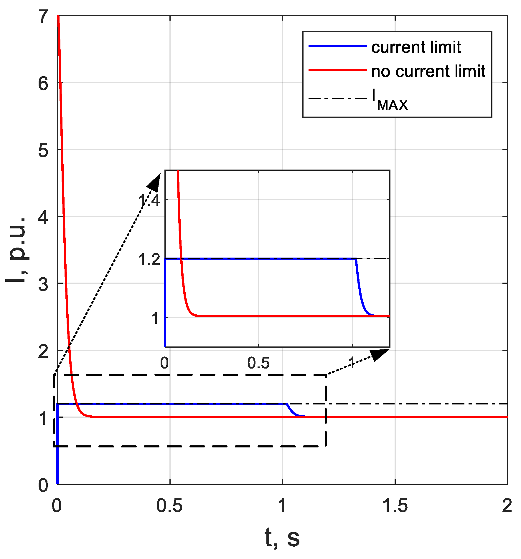
• To address the aforementioned issues, this manuscript investigates the transient stability of grid-forming converters in the post-fault period. The dynamic performance of the grid-forming converter changes under current saturation, which is analyzed in this manuscript by large-signal modelling and by considering current saturation, and provides a theoretical basis for subsequent optimization of the control strategy.
• In order to reduce the impact on the grid during the post-fault period, and in order to avoid instability, several restart strategies are proposed, such as a voltage zero-crossing start and an auxiliary synchronization strategy. In addition, control methods based on variable control parameters are proposed. The use of these strategies avoids putting the converter into current saturation during post-fault periods and allows for an increased rate of resynchronization and the speed up of the active power recovery after the restart to assist the grid in restoring active power balance.

The remaining sections of this manuscript are organized as follows: Section 2 will provide an introduction to the grid-forming’s control strategy with a large-signal modelling and dynamic performance investigation of the converter in the current saturation case. Section 3 will investigate the dynamic characteristics of the converter during a fault, especially post-fault, and propose several restart strategies. In Section 4, the above findings and optimization strategies are validated by a joint controller hardware-in-the-loop test system. Section 5 concludes the full manuscript.

2. Large-Signal Analysis of the Grid-Forming Converter

In this section, the control strategies of the grid-forming converter are described. It also presents a large-signal modelling and investigation of the control loop responsible for synchronization: the active power-frequency (P-f) control loop. The investigation focuses on the comprehensive comparison between system behaviour with neglected current saturation and with current saturation considered.

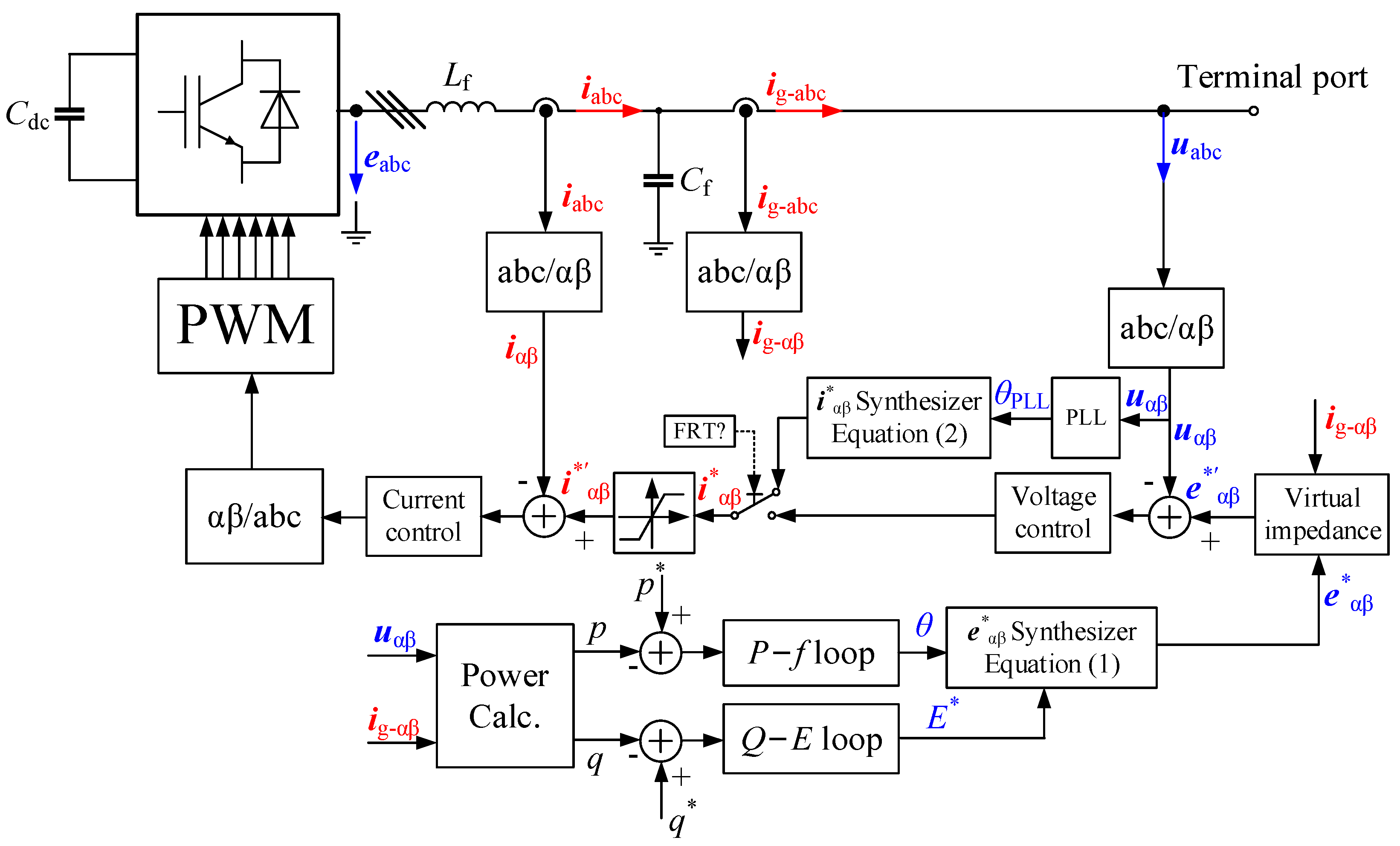
2.1. Control Strategies

A simplified grid-forming converter-grid system consisting of a converter (power semiconductors), EMI filter, grid impedance, and public grid is illustrated in Figure 1. A detailed description of the model used as well as a deviation of the relevant set of equations is given in [8]. As the focus of this investigation is on the grid connection side, the DC side of the converter as well as the energy source are simplified to a constant DC voltage source.

In Figure 1, the voltage $\underset{\_}{E}$ at B1 is the equivalent output voltage of the power semiconductor’s circuit. $\underset{\_}{I}$ is the output current of the converter. ${\underset{\_}{Z}}_{\mathrm{f}}$ is the filter impedance. The voltage $\underset{\_}{U}$ at B2 is the terminal port voltage. The voltage ${\underset{\_}{V}}_{\mathrm{g}}$ at B3 is the public grid voltage.

The control of the grid-forming converter in this manuscript is based on the αβ axis, as illustrated in Figure 2. Therefore, quasi-proportional resonance (PR) controllers [4] are used for the internal loop control of the voltage and current, in order to control the sinusoidal signal without static errors. Furthermore, the control in this manuscript is based on per unit values.

In Figure 2, the grid voltage ${\mathit{u}}_{\mathrm{abc}}$ and the grid current ${\mathit{i}}_{\mathrm{g}-\mathrm{abc}}$ are converted into ${\mathit{u}}_{\mathsf{\alpha }\mathsf{\beta }}$ and ${\mathit{i}}_{\mathrm{g}-\mathsf{\alpha }\mathsf{\beta }}$, respectively, by the abc/αβ transformation. The output active and reactive power of the converter p and q, respectively, can then be calculated. The active and reactive powers are compared with reference values and their deviations are fed into the P-f loop and the Q-E loop, respectively, in order to produce the reference phase angle θ and the reference voltage amplitude $E^{*}$. The reference voltage amplitude and the reference phase are synthesized via (1) into the αβ component of the reference voltage

$$\{\begin{array}{l}{e}_{\alpha }^{*}=E^{*}\cos \left(\theta \right)\\ e_{\beta }^{*}=E^{*}\sin \left(\theta \right)\end{array}.$$

(1)

The robustness of the converter is improved by the virtual impedance, which generates the reference value ${\mathit{e}}_{\mathsf{\alpha }\mathsf{\beta }}^{*\prime }$ for voltage loop control. A quasi-PR controller regulates the voltage and calculates the reference value ${\mathit{i}}_{\mathsf{\alpha }\mathsf{\beta }}^{*\prime }$ for current loop control. Due to the low current-carrying capacity of the power semiconductor components, even a short period of overcurrent can permanently damage the semiconductor components. In order to protect the converter, the current reference amplitude must therefore be restricted by a limit controller. Another quasi-PR controller regulates the current; the generated reference voltage is converted through αβ/abc transformation. The power electronics of the converter are controlled by a PWM modulation unit.

In order to meet the requirements for reactive current injection in a negative sequence [23], the double second-order generalized integrator (DSOGI)-based PLL [24,25] is used during the fault. Thus, when a fault is detected, the current loop control uses the reference current generated by (2) with the assistance of the DSOGI-PLL directly, while disconnecting the reference currents from the P-f and Q-E loops and the voltage loop control.

$$\{\begin{array}{l}{i}_{\mathsf{\alpha }}^{*}=\sqrt{i_{\mathrm{d}}^{*}{}^2+i_{\mathrm{q}}^{*}{}^2}\cos \left({\theta }_{\mathrm{PLL}}+{\tan }^{-1}\left(\frac{i_{\mathrm{q}}^{*}}{i_{\mathrm{d}}^{*}}\right)\right)\\ i_{\mathsf{\beta }}^{*}=\sqrt{i_{\mathrm{d}}^{*}{}^2+i_{\mathrm{q}}^{*}{}^2}\sin \left({\theta }_{\mathrm{PLL}}+{\tan }^{-1}\left(\frac{i_{\mathrm{q}}^{*}}{i_{\mathrm{d}}^{*}}\right)\right)\end{array}$$

(2)

The reference currents $i_{\mathrm{d}}^{*}$ and $i_{\mathrm{q}}^{*}$ herein come from the grid codes [23].

During a fault, the converter therefore operates in a similar way to the grid following mode. After the fault clearing, the converter returns to the grid-forming mode, i.e., the reference currents of the current loop control are derived from the P-f and Q-E loops as well as the voltage loop control.

In order to further investigate the dynamic characteristics of the grid-forming converter, in particular the synchronous performance, large-signal modelling is carried out with the P-f loop as the main component. Since the Q-E loop can practically be decoupled from the P-f loop [15], which is not taken into account in this investigation, it is considered as an ideal unit in large-signal modelling. Furthermore, since the control bandwidth of the voltage and current loops is often at least one order of magnitude larger than that of the P-f loop, they are assumed to be ideal gain units [12] in large-signal modelling and subsequent investigations.

The most common P-f loop control strategies available today are droop-like control [8,20] and virtual synchronous generator (VSG) control [12,17], as depicted in Figure 3.

Two of the common P-f control strategies currently available are illustrated in Figure 3. These are droop-like controls as presented in Figure 3a, and VSG as shown in Figure 3b. Since power synchronous control [8] and droop control are identical in a large-signal sense, this manuscript therefore treats them as the same type of control for the analysis.

In Figure 3a, by filtering the deviation between the active power reference $p^{*}$ and the instantaneous output active power p, the P-f loop can eliminate the effects of sensor noise as well as current harmonics. A first-order low-pass filter is used here. The filtered deviation is regulated by a droop factor $D_{\mathrm{p}}$ to produce the angular frequency $∆\omega$. To improve the dynamic performance of the system, the P-f loop also has a feedforward factor of the rated grid angular frequency ${\omega }_0$. Then final angular frequency $\omega$ is converted into the reference phase $\theta$ by an integration unit.

In Figure 3b, the VSG mimics the rotor equations of a synchronous generator. The deviation between the active power reference $p^{*}$ and the instantaneous output active power p is produced through the regulated production angular frequency $∆\omega$ of the damping factor D and the inertia factor H. The reference phase $\theta$ is subsequently obtained in a similar way to the droop control.

Under the assumption that the rated grid angular frequency ${\omega }_0$ is constant, the second-order differential equations for the droop control of Figure 3a and the VSG of Figure 3b are expressed as follows

$$\frac{{\mathrm{d}}^2}{\mathrm{d}{t}^2}\theta \left(t\right)=-{\omega }_{\mathrm{p}}\frac{\mathrm{d}}{\mathrm{d}t}\theta \left(t\right)+D_{\mathrm{p}}{\omega }_{\mathrm{p}}\left(p^{*}-p\left(t\right)\right),$$

(3)

$$\frac{{\mathrm{d}}^2}{\mathrm{d}{t}^2}\theta \left(t\right)=-\frac{D}{H}\frac{\mathrm{d}}{\mathrm{d}t}\theta \left(t\right)+\frac{1}{H}\left(p^{*}-p\left(t\right)\right).$$

(4)

The two Equations (3) and (4) are identical by setting (5)

$$\{\begin{array}{l}D=\frac{1}{D_{\mathrm{p}}}\\ H=\frac{1}{D_{\mathrm{p}}{\omega }_{\mathrm{p}}}\end{array}.$$

(5)

The droop control of Figure 3a and the VSG of Figure 3b are thus equivalent in a large-signal sense as long as (5) is satisfied. Therefore, the droop control with a first-order low-pass filter is used for subsequent investigations in this manuscript.

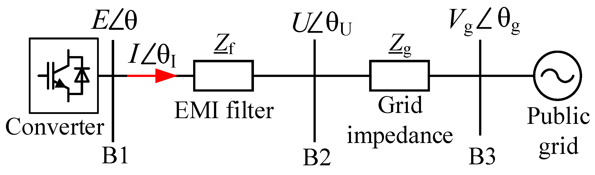
2.2. Current-Unsaturated Converter-Grid System

In order to protect the power semiconductor components, the output current amplitude must be limited to the converter’s maximum allowed physical limits. The limited current amplitude leads to a restricted active power output. This influences the dynamic characteristics of the P-f loop. Within the next two subsections, system behavior is investigated without current saturation and compared to system behavior with current saturation, respectively.

First, it is assumed that the converter never enters current saturation, i.e., the current amplitude threshold is infinite, to facilitate the analysis.

The active power output from B2 to the grid in Figure 1 is

$$p\left(t\right)=\frac{U^2\cos \left({\theta }_{\mathrm{Z}}\right)-V_{\mathrm{g}}U\cos \left({\theta }_{\mathrm{U}}\left(t\right)+{\theta }_{\mathrm{Zg}}\right)}{\left|{\underset{\_}{Z}}_{\mathrm{g}}\right|}.$$

(6)

Substitute (6) into (3) and set

$$\{\begin{array}{l}x\left(t\right)={\theta }_{\mathrm{U}}\left(t\right)\\ y\left(t\right)=\frac{\mathrm{d}}{\mathrm{d}t}{\theta }_{\mathrm{U}}\left(t\right)\end{array},$$

(7)

in order to obtain a set of two first-order differential equations

$$\{\begin{array}{l}\frac{\mathrm{d}}{\mathrm{d}t}x\left(t\right)=y\left(t\right)\\ \frac{\mathrm{d}}{\mathrm{d}t}y\left(t\right)=-{\omega }_{\mathrm{p}}y\left(t\right)+D_{\mathrm{p}}{\omega }_{\mathrm{p}}\frac{V_{\mathrm{g}}U}{\left|{\underset{\_}{Z}}_{\mathrm{g}}\right|}\cos \left(x\left(t\right)+{\theta }_{\mathrm{Zg}}\right)+D_{\mathrm{p}}{\omega }_{\mathrm{p}}\left(p^{*}-\frac{U^2}{\left|{\underset{\_}{Z}}_{\mathrm{g}}\right|}\cos \left({\theta }_{\mathrm{Zg}}\right)\right)\end{array}.$$

(8)

In order to obtain the stable equilibrium point (SEP) of (8) [36], assume the SEP is located in $(x_0, y_0)$ of the phase plane. The SEP’s coordinates are characterized in the following: $x_0$, phase of converter terminal voltage; $y_0$, instantaneous angular frequency ($y=\frac{\mathrm{d}{\theta }_U}{\mathrm{dt}}{|}_{t=0}$).

$$\{\begin{array}{l}0=y_0\\ 0=-{\omega }_{\mathrm{p}}{y}_0+D_{\mathrm{p}}{\omega }_{\mathrm{p}}\frac{V_{\mathrm{g}}U}{\left|{\underset{\_}{Z}}_{\mathrm{g}}\right|}\cos \left(x_0+{\theta }_{\mathrm{Zg}}\right)+D_{\mathrm{p}}{\omega }_{\mathrm{p}}\left(p^{*}-\frac{U^2}{\left|{\underset{\_}{Z}}_{\mathrm{g}}\right|}\cos \left({\theta }_{\mathrm{Zg}}\right)\right)\end{array}.$$

(9)

Two equilibrium points (EPs) can be obtained from (9)

$$x_0=\pm {\cos }^{-1}\left(\frac{U^2\cos \left({\theta }_{\mathrm{Zg}}\right)-\left|{\underset{\_}{Z}}_{\mathrm{g}}\right|p^{*}}{U{V}_{\mathrm{g}}}\right)-{\theta }_{\mathrm{Zg}}+n2\pi ,\begin{array}{cc}& n\in Z\end{array}.$$

(10)

To determine the stability of these two EPs, substitute (10) into (8)

$$\{\begin{array}{l}{f}_1\left(x_0,y_0\right)=y_0\\ f_2\left(x_0,y_0\right)=-{\omega }_{\mathrm{p}}{y}_0+D_{\mathrm{p}}{\omega }_{\mathrm{p}}\frac{V_{\mathrm{g}}U}{\left|{\underset{\_}{Z}}_{\mathrm{g}}\right|}\cos \left(x_0+{\theta }_{\mathrm{Zg}}\right)+D_{\mathrm{p}}{\omega }_{\mathrm{p}}\left(p^{*}-\frac{U^2}{\left|{\underset{\_}{Z}}_{\mathrm{g}}\right|}\cos \left({\theta }_{\mathrm{Z}}\right)\right)\end{array}.$$

(11)

Its Jacobian matrix at the EPs $(x_0, y_0)$ is

$$\mathbf{J}=\left[\begin{array}{cc}\frac{\partial f_1}{\partial x_0}& \frac{\partial f_1}{\partial y_0}\\ \frac{\partial f_2}{\partial x_0}& \frac{\partial f_2}{\partial y_0}\end{array}\right]=\left[\begin{array}{cc}0& 1\\ -D_{\mathrm{p}}{\omega }_{\mathrm{p}}\frac{V_{\mathrm{g}}U}{\left|{\underset{\_}{Z}}_{\mathrm{g}}\right|}\cos \left(x_0+{\theta }_{\mathrm{Zg}}\right)& -{\omega }_{\mathrm{p}}\end{array}\right].$$

(12)

In order for the system to be stable, the real part of the eigenvalues of the J matrix must be negative. This leads to the criterion that

$$-{\theta }_{\mathrm{Zg}}\le x_0\le \mathsf{\pi }-{\theta }_{\mathrm{Zg}}.$$

(13)

According to the criterion (13), the stable equilibrium point is obtained as

$$x_{\mathrm{SEP}}={\cos }^{-1}\left(\frac{U^2\cos \left({\theta }_{\mathrm{Zg}}\right)-\left|{\underset{\_}{Z}}_{\mathrm{g}}\right|p^{*}}{U{V}_{\mathrm{g}}}\right)-{\theta }_{\mathrm{Zg}}+n2\pi ,$$

(14)

where $n2\pi$ implies the existence of periodic SEPs. Furthermore, in order for a physically meaningful SEP, $x_{\mathrm{SEP}}$ must be real, and thus the active power reference must satisfy (15)

$$p^{*}\le \frac{V_{\mathrm{g}}U+U^2\cos \left({\theta }_{\mathrm{Zg}}\right)}{\left|{\underset{\_}{Z}}_{\mathrm{g}}\right|}.$$

(15)

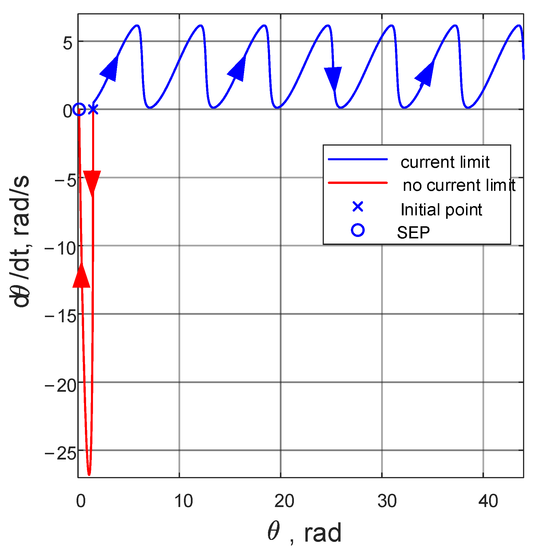
2.3. Current-Saturated Converter-Grid System

With reference to Figure 1, when the output current reaches the maximum value of the allowed current amplitude, $I_{\max }$, the active power output of the converter is

$$p\left(t\right)=I_{\max }U\cos \left({\theta }_{{\rm I}}\left(t\right)\right).$$

(16)

The second-order non-linear differential Equation (17) for the converter-grid system in the case of current saturation is obtained by substituting (16) into (3)

$$\frac{{\mathrm{d}}^2}{\mathrm{d}{t}^2}\theta \left(t\right)=-{\omega }_{\mathrm{p}}\frac{\mathrm{d}}{\mathrm{d}t}\theta \left(t\right)+D_{\mathrm{p}}{\omega }_{\mathrm{p}}\left(p^{*}-I_{\max }U\cos \left({\theta }_{{\rm I}}\left(t\right)\right)\right).$$

(17)

Its stable equilibrium point can be obtained by a similar method as in Section 2.1

$$x_{\mathrm{SEP}}^{\prime }={\cos }^{-1}\left(\frac{p^{*}}{I_{\max }U}\right)+n2\pi .$$

(18)

It is worth noting that its stable equilibrium point and the grid impedance are no longer relevant as in (14). In order for a real number of SEP to exist, the active power reference needs to satisfy (19)

$$p^{*}\le I_{\max }U.$$

(19)

In total, the system is described for both unsaturated and saturated currents by (20)

$$\begin{array}{l}\frac{{\mathrm{d}}^2}{\mathrm{d}{t}^2}\theta \left(t\right)=-{\omega }_{\mathrm{p}}\frac{\mathrm{d}}{\mathrm{d}t}\theta \left(t\right)+D_{\mathrm{p}}{\omega }_{\mathrm{p}}\left(p^{*}-p\left(t\right)\right)\\ \{\begin{array}{c}p\left(t\right)=\frac{U^2\cos \left({\theta }_{\mathrm{Z}}\right)-V_{\mathrm{g}}U\cos \left({\theta }_{\mathrm{U}}\left(t\right)+{\theta }_{\mathrm{Zg}}\right)}{\left|{\underset{\_}{Z}}_{\mathrm{g}}\right|}\begin{array}{cc}& \mathrm{unsaturated}\end{array}\\ p\left(t\right)=I_{\max }U\cos \left({\theta }_{{\rm I}}\left(t\right)\right)\begin{array}{cccc}\begin{array}{ccc}\begin{array}{cc}& \end{array}& & \end{array}& & & \mathrm{saturated}\end{array}\end{array}\\ \end{array}$$

(20)

If current limiting is not taken into account, the dynamic performance of the converter will differ considerably from the real situation, i.e., a current-limited system. The trajectories of these two systems are obtained by solving the differential Equations (8) and (20) in the time domain, as illustrated in the phase portrait in Figure 4. As the investigation of the dynamic characteristics of the system in this manuscript is qualitative rather than quantitative, the uncertainty of the control parameters is not investigated.

As illustrated in Figure 4, the red curve is the trajectory without current limitation and the blue curve is the trajectory with current limitation. The blue x is the position of the initial operation point. The blue o represents the SEP. After the system is started, the operation point reaches the SEP along the red and blue curves, respectively.

Since the current is not limited, the deviation between the reference active power and the actual active power in (6) are also not limited; thus, the movement of the operation point in the $d\theta /dt$ direction is not limited. This implies that the operation point can return to the SEP quickly along the red curve, as also shown in Figure 5. In Figure 5, the output current amplitude without current limitation (red curve) instantaneously reaches 7 p.u. after start-up and then returns to 1.0 p.u. within 0.2 s, i.e., the operation point reaches its stable equilibrium point.

With current limitation, the trajectory (blue curve in Figure 4) overlaps with the trajectory without current limitation (red curve in Figure 4) within a short time after start-up. During this period, the current amplitude remains below $I_{\max }$. When the current amplitude rapidly reaches $I_{\max }$, as depicted in the blue curve in Figure 5, the system enters the current saturation state. The deviation in active power $∆p$ in (17) is therefore constrained to be

$$\left|\Delta p\right|\le \left|\pm 1-I_{\max }\right|U.$$

(21)

In Figure 4, the blue curve representing the current-limited system is limited in its change in the $d\theta /dt$ direction, implying that the operation point takes more time to return to the SEP along the blue curve. In Figure 5, the output current amplitude of the current-limited system (blue curve) momentarily reaches 1.2 p.u., the maximum allowed current amplitude, $I_{\max }$, after the system starts. It then remains at $I_{\max }$ for about 1 s before falling back to 1.0 p.u.

When the current amplitude is less than $I_{\max }$, the system exits current saturation. Therefore, in Figure 4, the trajectory of the current-limited system on the left (blue curve) and the trajectory of the system without current limitation (red curve) overlap again.

The dynamic performance of the current-limited system is considerably worse than that of the system without current limitation by using the same control parameters. According to (21), the dynamic performance becomes slower as $I_{\max }$ decreases.

Due to the difference in the differential equations, the domain of attraction (DOA) [37] of the current-limited system is shifted compared to the current-limited system, as illustrated in Figure 6.

In Figure 6, the differently colored blocks represent different areas of the DOA. All operation points located in the yellow area can return to the original SEP point. All operation points located in the green area can return to $\mathrm{SEP}-2\mathsf{\pi }$, which is the neighboring SEP on the left. The operation points located in the orange area can return to $\mathrm{SEP}+2\mathsf{\pi }$, which is the neighboring SEP on the right.

In the current-unsaturated system (Figure 6 top), the DOA is symmetrically distributed left and right, centered on the SEP. In the current-saturated system (Figure 6 bottom), the DOA is shifted to the left overall. This results in the right-hand DOA boundary being closer to the SEP, making the operation point prone to move to the neighboring SEP on the right.

For the same initial operation point $(\mathrm{SEP}+0.44\mathsf{\pi }, 0)$, its trajectory is quite different for the two systems. In the current-unsaturated system (Figure 6 top) the initial operation point * is located in the yellow area, so it follows the red curve back to the original SEP. Meanwhile, in the current-saturated system (Figure 6 bottom), the initial operation point * is located in the orange area. It therefore follows the blue curve to the neighboring SEP on the right.

Figure 7 illustrates the current amplitude curves for the same initial operation point in different systems. The red curve depicts the current amplitude of a current-unsaturated system and the blue curve depicts the current amplitude for a current-saturated system. Similar to Figure 5, the current amplitude of the current-unsaturated system (red curve) rises to 11 p.u. directly after start-up, then drops back and stabilizes at 1.0 p.u. after 0.2 s.

The current amplitude of the current-saturated system (blue curve), on the other hand, will experience a longtime interval taking on negative values before the active power returns to 1.0 p.u. if the operation point moves from left to right towards the neighboring SEP, as illustrated in Figure 6. Long periods of negative power output are unfavorable for the stable operation of either the converter or the grid system and should be avoided. This will be investigated in detail in the next section.

In summary, the dynamic performance of a current-unsaturated system differs significantly from that of a current-saturated system. Since a realistic converter must limit its current amplitude, it is important to use systems that take current limitation into account when investigating the transient performance of grid-forming converters.

3. Investigation of Dynamic Performance during and after Fault

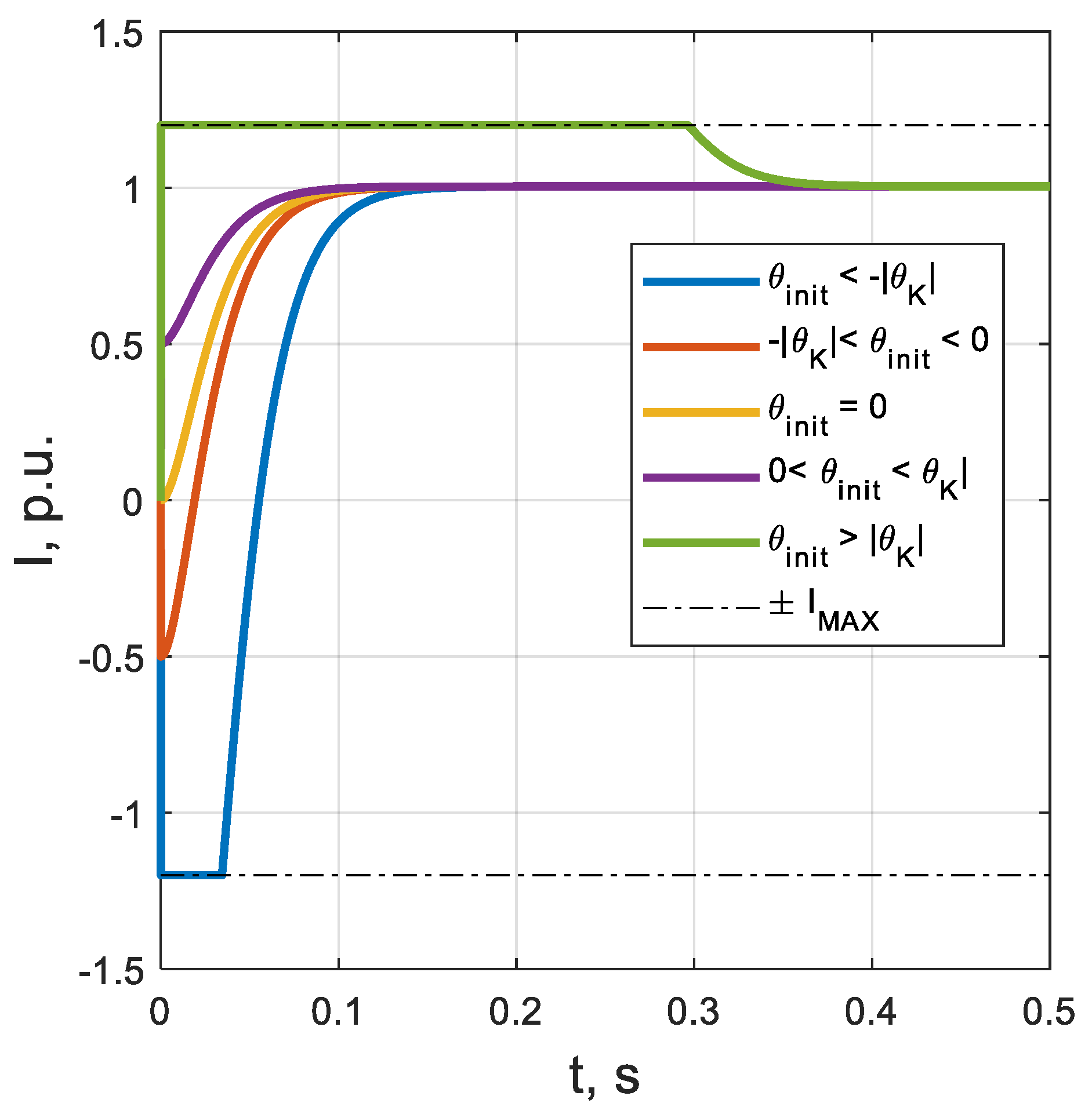
3.1. During a Fault

To make the system’s SEP of the reference active power exist, the thresholds (15) and (19) are rewritten and the terminal voltage amplitude ($U$) is set to follow the grid voltage ($V_g$) exactly. The thresholds for the terminal voltage amplitudes of the two systems are derived separately as follows

$$U\ge \sqrt{\frac{p^{*}\left|{\underset{\_}{Z}}_{\mathrm{g}}\right|}{1+\cos \left({\theta }_{\mathrm{Zg}}\right)}},$$

(22)

$$U\ge \frac{p^{*}}{I_{\max }}.$$

(23)

When the terminal voltage amplitude satisfies (22) and (23), respectively, an SEP exists. When a grid fault occurs, the terminal voltage amplitude drops, and an SEP does not exist when it falls below the threshold. As a result, the system diverges and the converter loses synchronization.

For an exemplary investigation of voltage thresholds, an active power reference of 1 p.u. is assumed. In an overhead lines dominated grid, the inductance dominates the grid impedance, so the denominator in (22): $(1+\cos \left({\theta }_{\mathrm{Zg}}\right)$ is approximately 1. From this, the terminal voltage threshold for a system without a current limit is proportional to the root of the grid impedance. For example, when the grid impedance is 0.1 p.u., the terminal voltage’s threshold is approximately 0.32 p.u. In contrast, the terminal voltage threshold for a current limit system is only related to the maximum current amplitude. When $I_{\max }=1.2 \mathrm{p}.\mathrm{u}.$, the terminal voltage threshold is approximately 0.83 p.u.

When a grid fault occurs, and the residual voltage at the terminal point falls below 0.83 p.u., there will be no SEP in the current limit system. Thus, the system cannot be stabilized, as illustrated in Figure 8.

In Figure 8, the red curve represents the trajectory on the phase portrait of a system without current limitation. The blue curve represents the trajectory of a system with current limitation. When a slight grid fault occurs, the residual voltage at the terminal port temporarily drops to 0.8 p.u. Since this voltage is still above the threshold for a system without current limitation (0.32 p.u.), its trajectory (red curve) converges rapidly to the SEP after starting from the initial point x. However, this voltage is less than the threshold for a current limit system (0.83 p.u.), so no SEP exists. The operation point continues to move to the right. During a fault, the system loses synchronization and the P-f loop is unable to provide an accurate reference phase. The converter, therefore, is also not able to deliver stable power.

However, in order to obtain an accurate reference phase during a fault, a backup PLL can be activated to generate a reference phase to replace the P-f loop. Furthermore, after the fault clearing, undesired phase oscillations and the resulting power oscillations can occur if the operation point is located far away from the SEP. To avoid these oscillations, the P-f loop can be frozen during the fault [38,39] and activated again after the fault clearing.

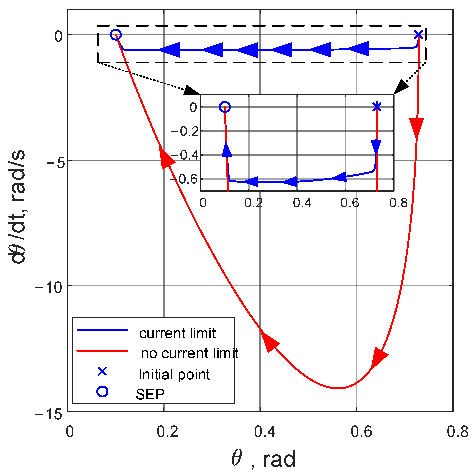
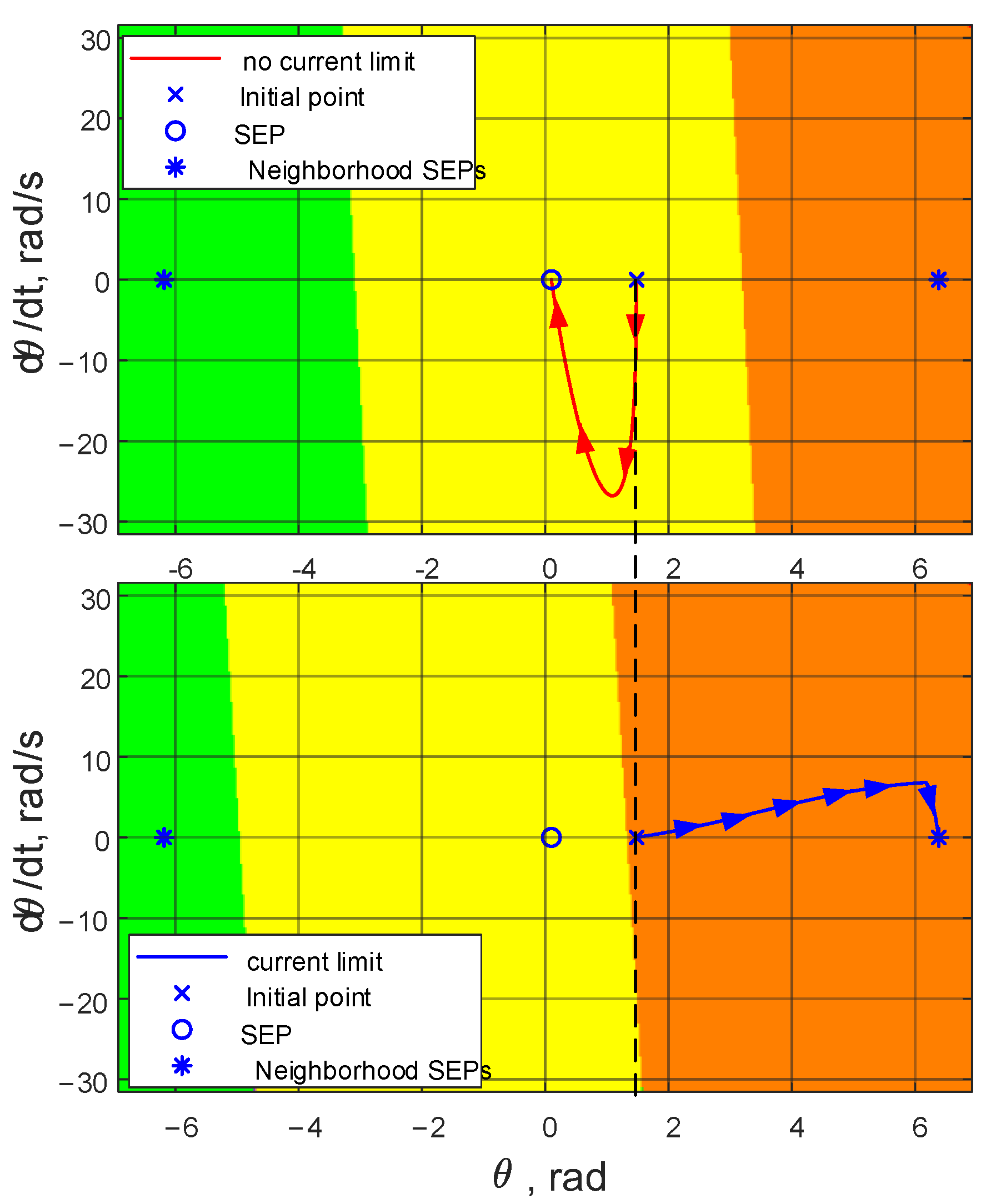
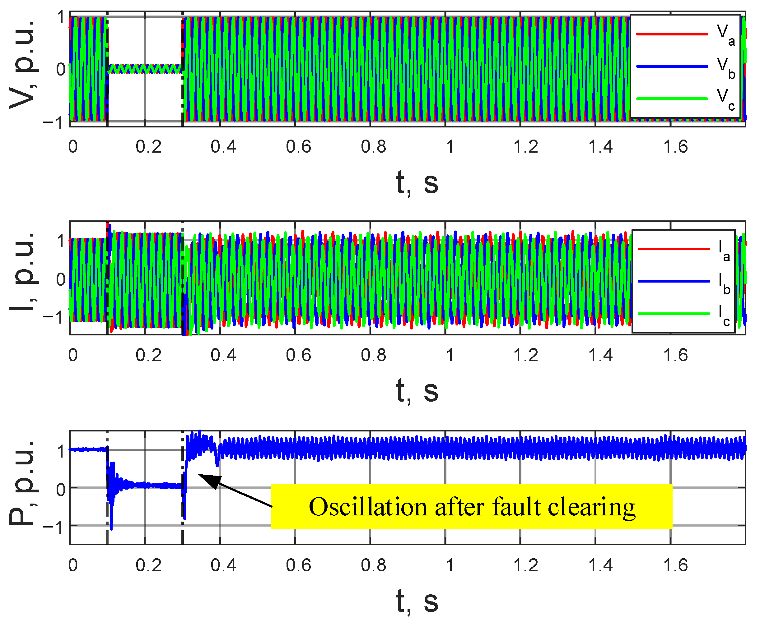
3.2. Post-Fault Clearing

This subsection investigates the dynamic characteristics of the converter after fault clearing. Unlike when the converter is black-started [27,28], after the fault clearing, the converter cannot use a synchronous switch to reduce its impact on the grid and the converter itself. Therefore, the initial operation point of the converter after the fault clearing will determine the dynamic characteristics of the converter.

After fault clearing, the terminal voltage is assumed to recover to 1.0 p.u. In strong grids, the terminal voltage is almost constant, while the voltage output of the converter varies according to its control strategy. Therefore, the dynamics of the P-f loop at the moment after the fault clearing is determined mainly by the voltage difference between B1 (power semiconductor’s circuit) $\underset{\_}{E}$ and B2 (terminal port) $\underset{\_}{U}$ and the filter impedance ${\underset{\_}{Z}}_{\mathrm{f}}$, as illustrated in Figure 1.

The initial equivalent voltage amplitude at B1 is $E=1.0 \mathrm{p}.\mathrm{u}.$ The voltage amplitude at terminal port $U$ is also $1.0 \mathrm{p}.\mathrm{u}$. The output current amplitude of the converter is then only influenced by the phase difference between $\underset{\_}{E}$ and $\underset{\_}{U}$, and the filter impedance ${\underset{\_}{Z}}_{\mathrm{f}}$, i.e.,

$$I=\frac{1}{\left|{\underset{\_}{Z}}_{\mathrm{f}}\right|}\sqrt{2-\cos \left(\theta -{\theta }_{\mathrm{U}}\right)}\le I_{\max }.$$

(24)

In order to avoid the P-f loop going into saturation during the post-fault period, and thus reducing its dynamic performance, it is necessary to ensure that the current amplitude is less than its maximum value, i.e., $I\le I_{\max }$, which can be achieved by making the reference phase lie within the threshold interval ${\theta }_{\mathrm{K}}$.

Associating the SEP (14) and (24) gives the phase threshold ${\theta }_{\mathrm{K}}$ (25) associated with the SEP. The threshold value of the phase ${\theta }_{\mathrm{k}}$ can be approximately expressed as

$${\theta }_{\mathrm{K}}\approx \pm I_{\max }\left|{\theta }_{\mathrm{SEP}}-{\theta }_{\mathrm{U}}\right|+{\theta }_{\mathrm{U}}.$$

(25)

To facilitate the investigation, the terminal voltage phase ${\theta }_{\mathrm{U}}$ is set to 0 here, which simplifies (25) into (26)

$${\theta }_{\mathrm{K}}\approx \pm I_{\max }\left|{\theta }_{\mathrm{SEP}}\right|.$$

(26)

This expresses that the phase threshold is proportional to the SEP with a scale factor of $I_{\max }$. In order that the P-f loop does not go into saturation when $I_{\max }=1.2 \mathrm{p}.\mathrm{u}.$, the initial phase and subsequent phases must not deviate beyond 1.2 times the SEP as illustrated in Figure 9.

In addition, in Figure 1, the active power output from B1 (power semiconductors circuit) to B2 (terminal port) is

$$p\left({\theta }_{\mathrm{init}}\right)=\frac{\cos \left({\theta }_{\mathrm{Zf}}\right)-\cos \left({\theta }_{\mathrm{init}}-{\theta }_{\mathrm{U}}+{\theta }_{\mathrm{Zf}}\right)}{\left|{\underset{\_}{Z}}_{\mathrm{f}}\right|}.$$

(27)

When ${\theta }_{\mathrm{init}}={\theta }_{\mathrm{U}}$, the initial active power is 0. If ${\theta }_{\mathrm{init}}<{\theta }_{\mathrm{U}}$, the initial active power is negative, as shown in Figure 9 and Figure 10.

In Figure 10, the three initial points within the threshold range (the three initial points between the two dashed lines in Figure 9) avoid current saturation and allow the active power to settle quickly at a given value.

The initial point of the green curve locates outside of the threshold range in Figure 9, so its current amplitude curve settles at the given value after saturation, as provided in Figure 10. The initial point of the blue curve is less than 0 and also locates outside of the threshold range in Figure 9. Thus, its current amplitude curve reaches a negative maximum value before returning to the given value.

For power generation converters, outputting negative active power can have a negative impact on the power balance of its DC link [36]. Excessive active power raises the DC link voltage and causes the DC link to cross the safety limit. During the fault, the DC link voltage is protected by the chopper circuit and stays near the voltage threshold. A further influx of energy into the DC link from the grid side will prevent the chopper circuit from continuing to absorb energy. This can lead to the DC link voltage crossing its safety limit, causing the converter to trip or even be damaged. In addition, the active power drawn from the grid by the generation equipment can have a serious negative impact on the stable operation of the grid.

Therefore, when restarting the P-f loop during the post-fault period, it is necessary to keep the initial phase close to ${\theta }_{\mathrm{U}}$, in order to reduce the impact of the initial current on the P-f loop, the converter, and the grid.

3.3. Post-Fault Restart Strategy

For ease of understanding, descriptions of the phases used in this section are provided in

Table 1. Description of different phases.

Phase	Description
${\theta }_{\mathrm{U}}$	Phase of the terminal voltage
${\theta }_{\mathrm{init}}$	Initial phase of the P-f loop at post-fault
${\theta }_{\mathrm{K}}$	Phase threshold to avoid current saturation
${\theta }_{\mathrm{P}-\mathrm{f}}$	Output reference phase of the P-f loop

.

After fault clearing, the terminal voltage phase ${\theta }_{\mathrm{U}}$ is influenced by the fault duration and the grid topology, which is largely unpredictable. As it is not possible to use synchronous switches, a software approach must be used to make the P-f loop’s initial phase ${\theta }_{\mathrm{init}}$ equal to ${\theta }_{\mathrm{U}}$. In addition, the active power output of the converter should be increased to its pre-fault value as soon as possible after fault clearing, in order to meet the requirements of grid frequency stability. Combining these two requirements, this subsection proposes several strategies for optimizing restarts at a post-fault period.

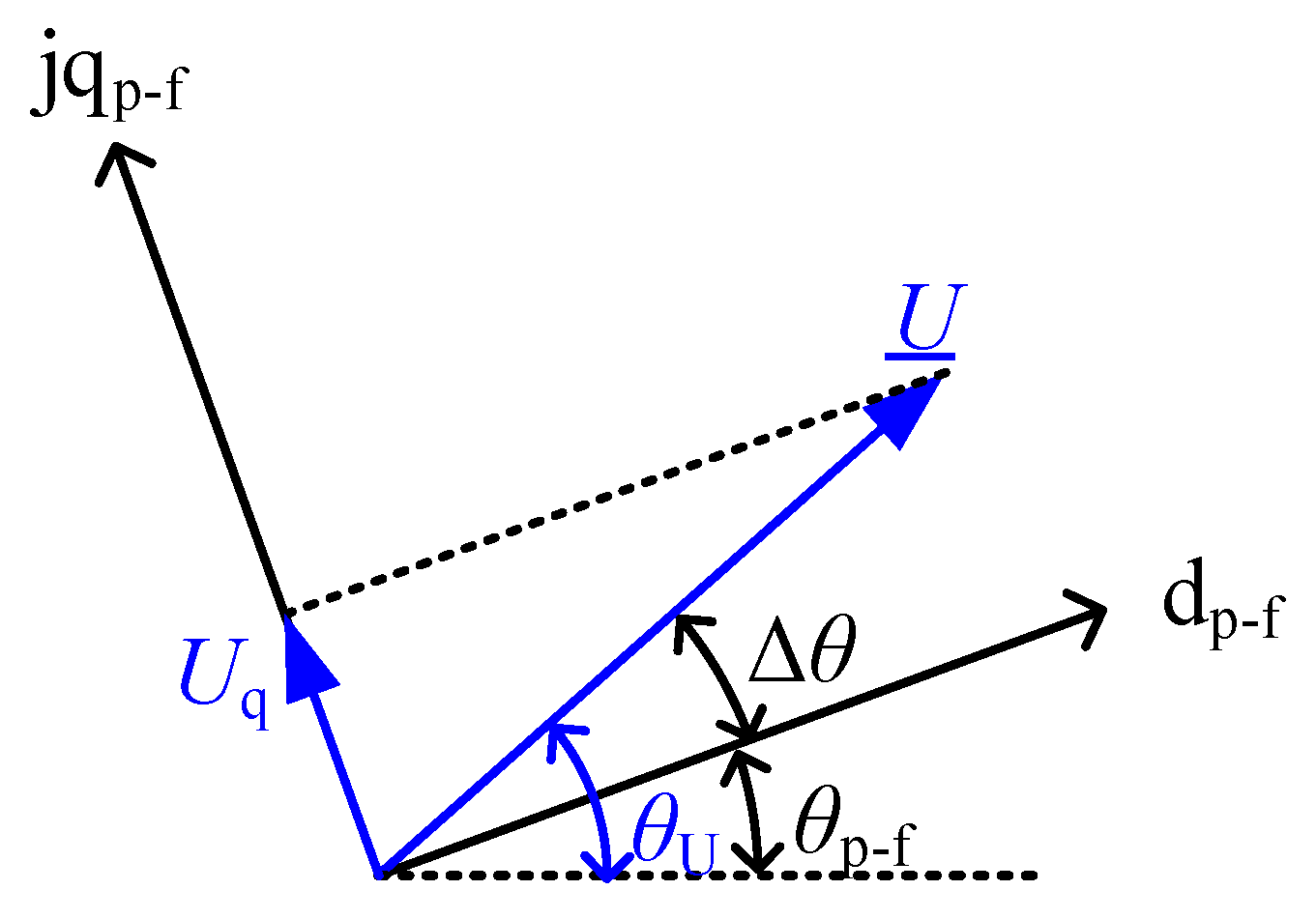
3.3.1. Restart with Voltage Zero-Crossing Detection

In order to avoid instabilities of the P-f loop due to a missing SEP, the P-f loop is frozen during the fault, then reset and restarted after fault clearing.

When the P-f loop is reset and restarted, its initial output phase is 0. When a terminal voltage’s rising edge passes the zero-crossing point, its phase ${\theta }_{\mathrm{U}}$ is also 0. Then a zero-crossing detection can simply achieve ${\theta }_{\mathrm{init}}={\theta }_{\mathrm{U}}=0$. Additionally, according to (27), the initial output power is 0.

To avoid interference with zero-crossing detection from temporary fluctuations in the terminal voltage during the post-fault period, zero-crossing detection should wait for the terminal voltage to stabilize. In engineering applications, zero-crossing detection is used with a low-pass filter to eliminate harmonic voltage interference. Usually this results in a phase delay that makes the detected zero-crossing point lag behind the actual one, i.e., ${\theta }_{\mathrm{init}}>{\theta }_{\mathrm{U}}$. However, according to the findings in Section 3.2, as long as this phase lag is not greater than the critical initial phase ${\theta }_{\mathrm{K}}$, no current saturation will occur. According to (25), when ${\theta }_{\mathrm{init}}>{\theta }_{\mathrm{U}}$, the output power is greater than 0, which allows the initial active power to be greater than 0.

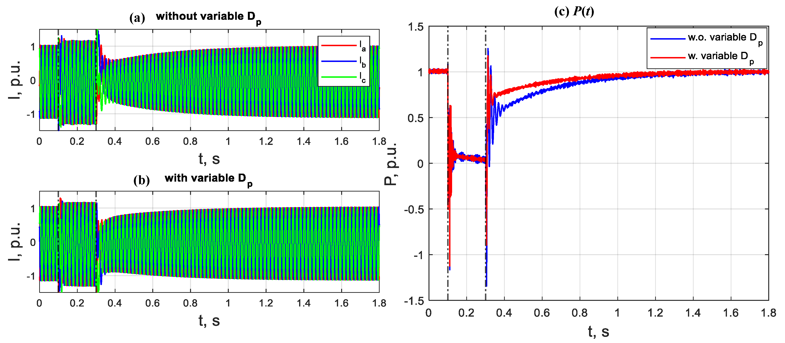
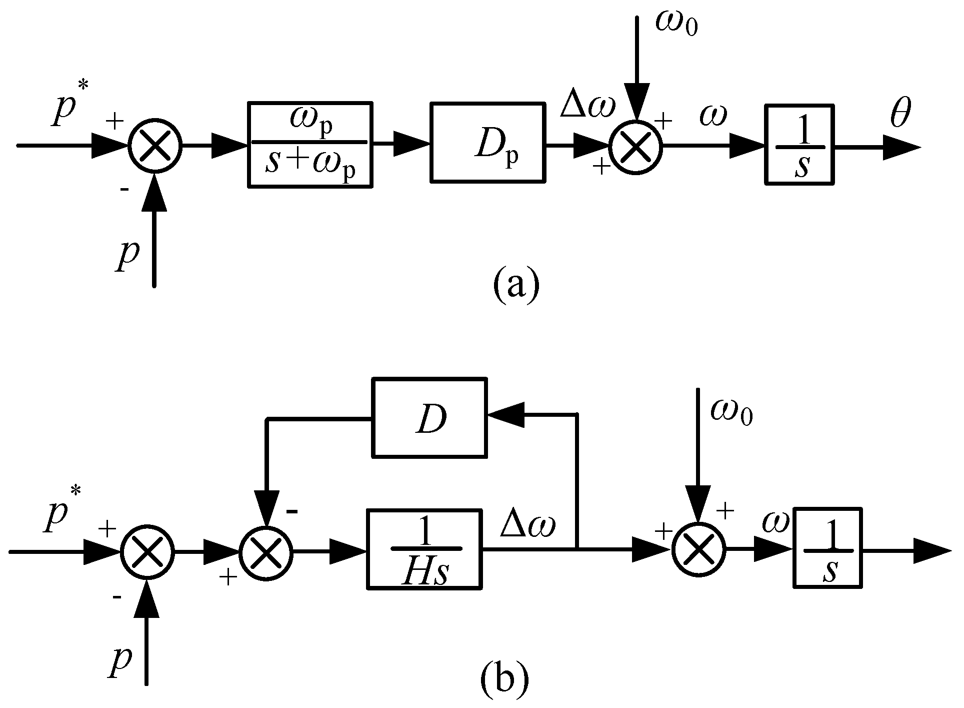
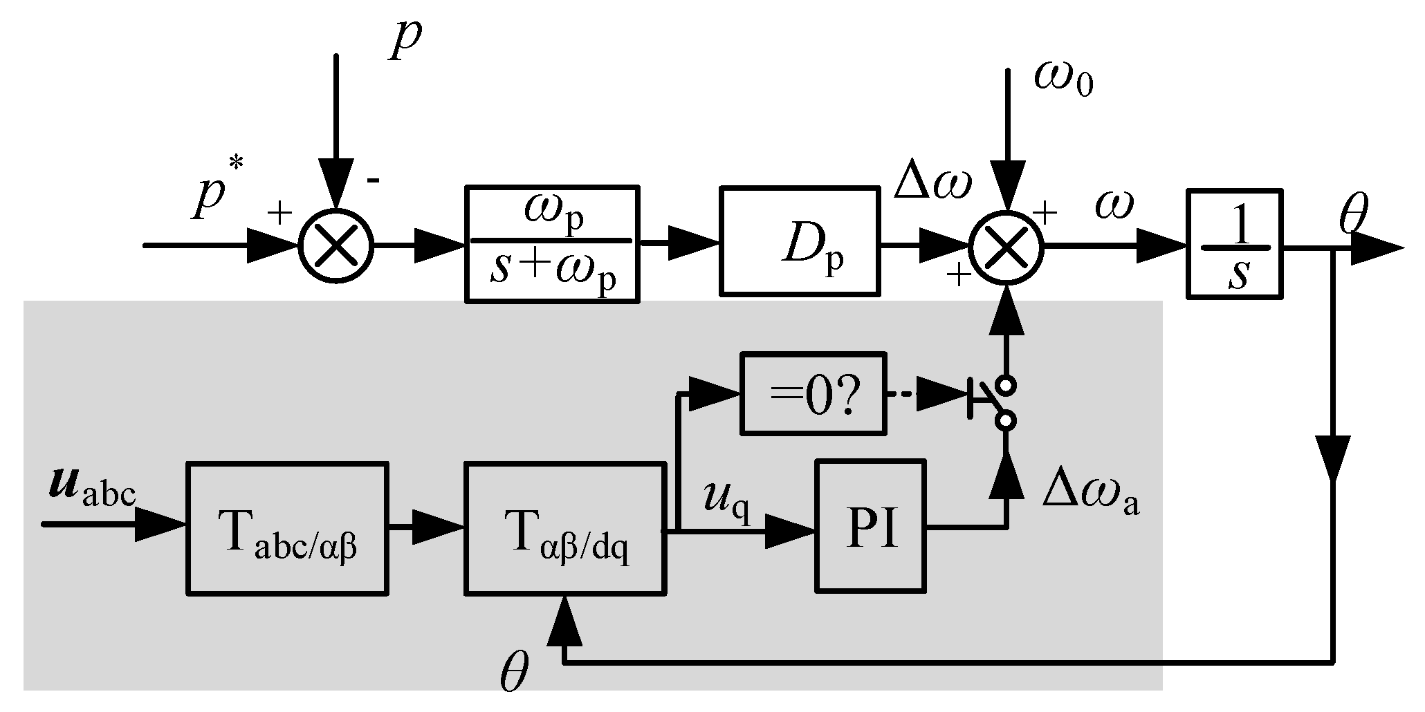
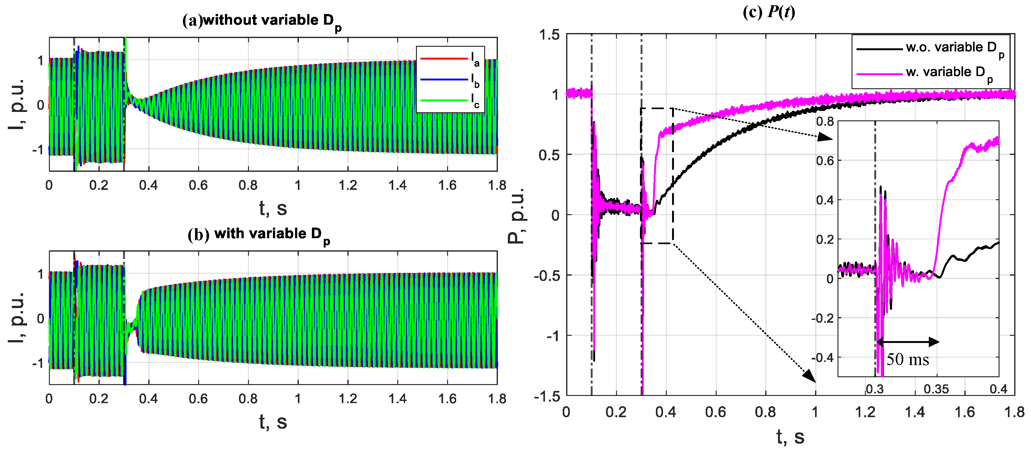
3.3.2. Restart with Variable Droop Factor $D_{\mathrm{p}}$

The dynamic performance of the P-f loop is related to the droop factor $D_{\mathrm{p}}$ and ${\omega }_{\mathrm{p}}$ in (3). With a constant ${\omega }_{\mathrm{p}}$, the higher the $D_{\mathrm{p}}$, the faster the dynamic performance of the P-f loop.

Restarting at a lower $D_{\mathrm{p}}$ during the post-fault period allows the P-f loop to avoid saturation and benefits small-signal stability [13]. However, the active power cannot reach the pre-fault value quickly. In modern power systems with an increasing share of converters, such a restart strategy would lead to an active power gap immediately after fault clearing and, consequently, to frequency stability problems. However, a large $D_{\mathrm{p}}$ will cause the current to go into saturation, which in turn reduces the dynamic performance of the P-f loop, and in addition, is not conducive to small-signal stability. This manuscript therefore proposes a variable $D_{\mathrm{p}}$ restart method.

After the P-f loop is reactivated, when the active power output is lower than a certain defined threshold, $D_{\mathrm{p}}$ is set to a larger value to quickly pull up the active power. When the active power is greater than this threshold, $D_{\mathrm{p}}$ is reduced to a normal value to ensure that no overshoot occurs and to avoid the P-f loop going into saturation, as illustrated in Figure 11 and Figure 12.

In Figure 11, the system is started with ${\theta }_{\mathrm{init}}={\theta }_{\mathrm{U}}=0$ at (0,0). The magenta curve represents the trajectory of the system with a constant $D_{\mathrm{p}}$ of 0.2 p.u./Hz. Due to the lower $D_{\mathrm{p}}$, the trajectory also changes less in the $\mathrm{d}\theta /\mathrm{d}t$ direction, which implies a slower dynamic performance.

When a variable $D_{\mathrm{p}}$ restart strategy is used, the blue curve in Figure 12 shows a $D_{\mathrm{p}}$ of 2 p.u./Hz before P reaches 0.4 p.u. Then the $D_{\mathrm{p}}$ is changed to 0.2 p.u./Hz as provided in the red curve in Figure 12. This system’s change in the $\mathrm{d}\theta /\mathrm{d}t$ direction is boosted by the larger $D_{\mathrm{p}}$. This can also be verified by the active power curve in Figure 12.

In Figure 12, the system with a constant $D_{\mathrm{p}}$ of 0.2 p.u./Hz, represented by the magenta curve, takes about 0.4 s to reach 1.0 p.u. The system with variable $D_{\mathrm{p}}$ reaches 1.0 p.u. after 0.04 s, and no overshoot or saturation occurs.

3.3.3. Restart with Auxiliary Synchronization

With the zero-crossing restart strategy, it is simple to achieve ${\theta }_{\mathrm{init}}={\theta }_{\mathrm{U}}$. However, this strategy requires a period of time after the fault clearing. This time period includes waiting for the terminal voltage to settle, waiting for the zero-crossing point to appear, etc. Therefore, for about 40 milliseconds after the fault clearing, there is no reference phase provided by the P-f loop, and the converter is therefore unable to deliver active power to the grid. This causes a short power gap to occur during the post-fault period. This is detrimental to the stable operation of the power system.

For this reason, this manuscript proposes an auxiliary synchronization strategy for the restart of the P-f loop.

As depicted in Figure 13, the terminal voltage vector $\underset{\_}{U}$ is located in the synchronous rotation coordinates of the P-f loop. After the fault clearing, there is a random phase difference $∆\theta$ between the terminal voltage phase ${\theta }_{\mathrm{U}}$ and the synchronous rotation coordinates’ phase ${\theta }_{\mathrm{P}-\mathrm{f}}$. Due to this phase difference $∆\theta$, the terminal voltage vector $\underset{\_}{U}$ maps a non-zero q-axis voltage component $U_{\mathrm{q}}$ on the q-axis; thus, $U_{\mathrm{q}}\ne 0$. In other words, if $U_{\mathrm{q}}=0$, the phase difference $∆\theta$ is zero, i.e., ${\theta }_{\mathrm{P}-\mathrm{f}}={\theta }_{\mathrm{U}}$.

Therefore, this manuscript uses a PLL-like method to quickly equalize ${\theta }_{\mathrm{U}}$ and the output angle of the P-f loop ${\theta }_{\mathrm{P}-\mathrm{f}}$ when the P-f loop is reactivated, as depicted in Figure 14.

Figure 14 illustrates the P-f loop containing the proposed auxiliary synchronization unit. A PLL-like control loop is in the gray box. The feedback signal of this control loop is the P-f loop’s output phase $\theta$. This phase is then used to obtain $U_{\mathrm{q}}$ by performing an abc/dq transformation of the terminal voltage. $U_{\mathrm{q}}$ is then adjusted to zero by a proportional integrator (PI) regulator, whose output signal is the auxiliary angular velocity $∆{\omega }_{\mathrm{a}}$.

The use of an auxiliary angular velocity instead of a direct auxiliary phase [34] avoids the sign jump in phase from $0–2\mathsf{\pi }$. This enhances the robustness of the system.

The $∆{\omega }_{\mathrm{a}}$ participates as a feedforward term to the control of the P-f loop after restarting, in order to achieve ${\theta }_{\mathrm{init}}={\theta }_{\mathrm{U}}$. This control loop is only activated for a short moment after the fault clearing: when $U_{\mathrm{q}}$ is not 0. After $U_{\mathrm{q}}\approx 0$, which means ${\theta }_{\mathrm{init}}\approx {\theta }_{\mathrm{U}}$, the auxiliary synchronization unit is inactive, so as to not affect the dynamic performance of the P-f loop and its small-signal stability performance.

In addition, this method can be applied simultaneously with the restart with variable $D_{\mathrm{p}}$ in order to further accelerate the recovery of active power.

In order to compare the three optimal control methods proposed in this manuscript,

Table 2. Comparison of the proposed methods.

Method	Advantages	Disadvantages
Zero-crossing start	Simple to implement, no control parameter tuning to consider	Slow recovery of active power after restart.
Start with variable droop factor	Fast resynchronization	Careful tuning of the parameters is required.
Start with auxiliary synchronization	Fast resynchronization	Additional control loops need to be added.

summarizes the advantages and disadvantages of the three methods.

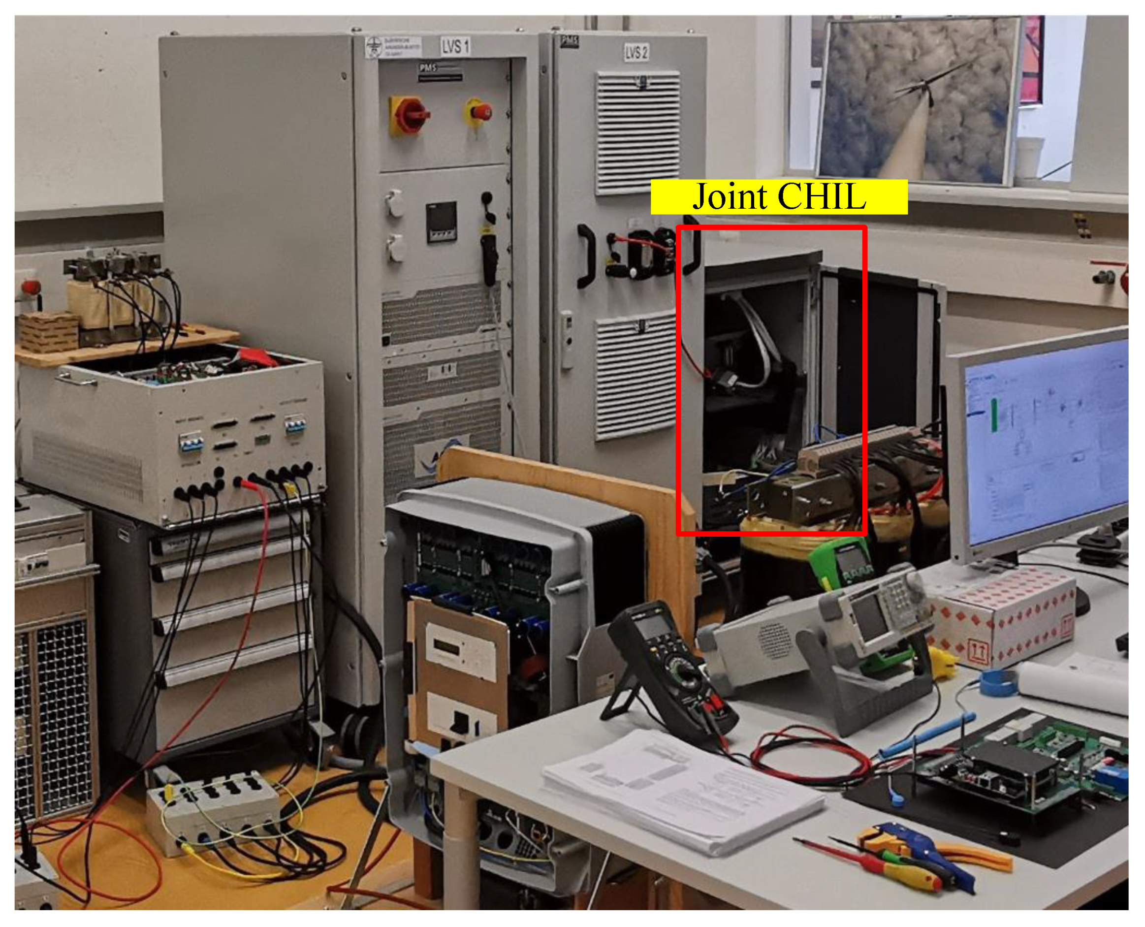
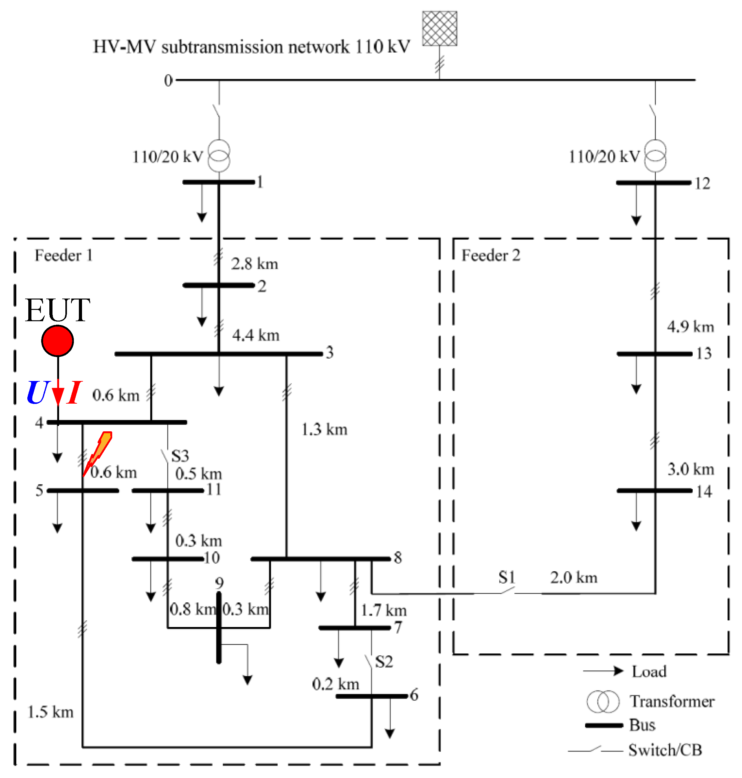
4. Test Verification

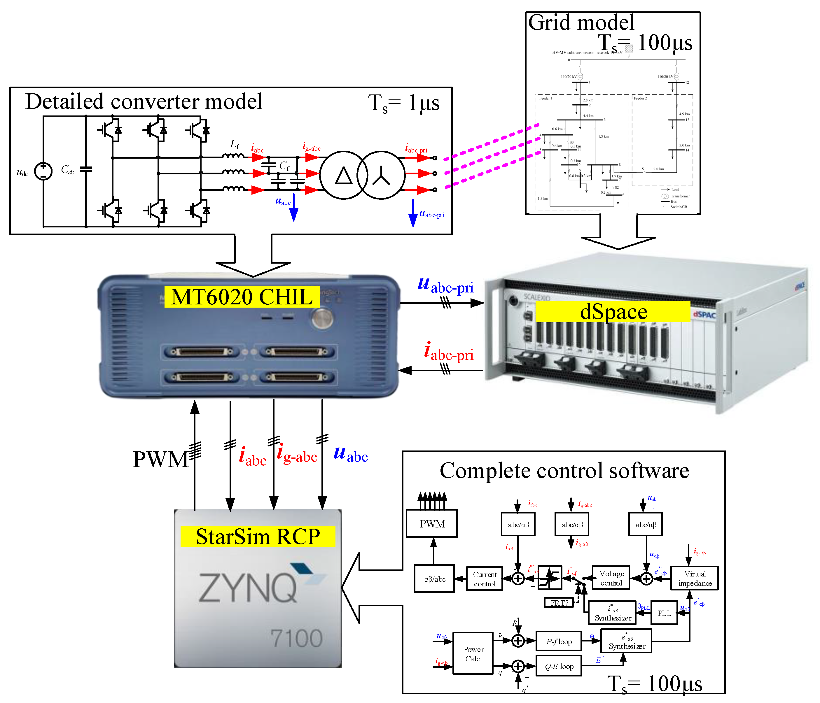
4.1. Test Setup

This section validates the findings of the previous sections and the control strategy. The tests were carried out with the joint controller hardware-in-the-loop (CHIL) [34] system in the laboratory.

Figure 15 shows a photo of the laboratory, in which the joint CHIL system is in the red box. The exact topology is outlined in Figure 16.

In Figure 16, the rightmost hardware device is the CPU-based real-time simulation system: dSpace SCALEXIO, in which the CIGRE European MV distribution network benchmark [40] grid model is deployed, as shown in Figure 17. The dSpace has a real-time simulation time step of 100 μs. This ensures the accuracy of the simulation at the medium voltage level.

In the FPGA-based controller hardware-in-the-loop test system: ModelingTech MT6020, a detailed converter model with IGBT components and a unit transformer, is deployed, as illustrated in the top middle of Figure 16. The MT6020 has a real-time simulation time step of 1 μs. This ensures an accurate simulation of the power electronics.

A StarSim rapid control prototyping (RCP), which includes he MT6020’s Xilinx Zynq-7100-based ARM processor, is provided below in Figure 16, where the complete converter control software is deployed, as provided in Figure 2. The calculation step in the StarSim RCP is 100 μs.

An analogue signal connection is used between the dSpace and the MT6020. In the grid model of dSpace, the equipment under test (EUT) is replaced by a controlled three-phase voltage source. The voltage signal comes from the primary side of the converter model in MT6020. In the converter model of MT6020, the grid model is replaced by a controlled three-phase current source, whose current signal comes from the terminal port in the dSpace’s grid model. In this way, models from two different hardware systems can be connected together virtually, as depicted in the three magenta dashed lines in Figure 16. With a similar setup to the power hardware-in-the-loop test [41], this joint CHIL system allows for both small-step real-time simulation of the converter and real-time simulation of the large-scale grid.

A communication bus connection is used in the MT6020 and its attached StarSim RCP. The MT6020 transmits voltage and current data from the converter model to the controller. It is processed by the software in the StarSim RCP and outputs PWM signals to the MT6020 to control the power electronics.

The grid model used for the joint CHIL test is illustrated in Figure 17. It comes from [40], an MV distribution network for the European region, which is fed by a 110 kV supply and two independent 110/20 kV transformers. In the test, the converter under test (EUT) is connected to bus 4, as shown by the red dot in Figure 17. All test results below are from the measurement point located on bus 4 to the EUT. As this manuscript focuses on investigating the dynamic characteristics of grid-forming converters after the fault clearing, a simple three-phase fault is set in the middle of the transmission line between bus 4 and bus 5, as presented by the lightning symbol in Figure 17. After 200 milliseconds of the fault, the transmission line between bus 4 and bus 5 is removed. Therefore, the fault duration is 200 milliseconds. During the test, the short circuit power of the 110 kV supply is set to 500 MVA to shape a slightly weaker grid, and thereby increase the challenge of the test. A detailed description of the specific parameters of this grid can be found in [40].

The hardware and control parameters of the converter are shown in

Table 3. Hardware parameters.

Name	Value
Rated power of the converter	1 MVA
Rated voltage of the converter	0.69 kV
Filter inductance	0.1 p.u.
Equivalent resistance on the filter	0.005 p.u.
Filter capacitance	0.33 p.u.
Ratio of the unit transformer	0.69/20 kV
Rated power of the unit transformer	1.25 MVA
Vector group of the unit transformer	Dy11
$u_{\mathrm{k}}$ of the unit transformer	6%

and

Table 4. Control parameters.

Name	Value
Droop factor of the P-f loop	0.2 p.u./Hz
Cut-off frequency of low-pass filter in P-f loop	20 Hz
Droop factor of the Q-E loop	1
Cut-off frequency of low-pass filter in Q-E loop	1 Hz
Control parameters of the backup PLL	$K_{\mathrm{P}-\mathrm{PLL}}=62$$, K_{\mathrm{I}-\mathrm{PLL}}=24$
Control parameters of the voltage loop	$K_{\mathrm{P}-\mathrm{V}}=2.8$$, K_{\mathrm{R}-\mathrm{V}}=102$
Control parameters of the current loop	$K_{\mathrm{P}-\mathrm{I}}=1.1$$, K_{\mathrm{R}-\mathrm{I}}=17.3$
Current amplitude threshold	1.2 p.u.
Control parameters of auxiliary synchronization	$K_{\mathrm{P}-\mathrm{AS}}=314$ and $K_{\mathrm{I}-\mathrm{AS}}=100$

.

4.2. Test Results and Analysis

In this subsection, the strategies mentioned in Section 3.3 are verified by the test configuration illustrated in Figure 16. The specific test cases are described in

Table 5. Test cases.

Numbering of Figures	Test Cases
Figure 18	No optimized control method
Figure 19	$\mathrm{Zero}-\mathrm{crossing} \mathrm{start} \mathrm{with} \mathrm{and} \mathrm{without} \mathrm{variable} D_{\mathrm{p}}$
Figure 20	$\mathrm{Zero}-\mathrm{crossing} \mathrm{start} \mathrm{with} \mathrm{variable} D_{\mathrm{p}}$$, \mathrm{auxiliary} \mathrm{synchronization} \mathrm{without} \mathrm{variable} D_{\mathrm{p}}$
Figure 21	$\mathrm{Auxiliary} \mathrm{synchronization} \mathrm{with} \mathrm{and} \mathrm{without} \mathrm{variable} D_{\mathrm{p}}$

. The test results are recorded by the recording function in the test system and plotted in parallel with the time of fault occurrence to facilitate comparative analysis.

In the test results illustrated in Figure 18, no restart optimization strategy is applied. In Figure 18, the upper figure shows the three-phase voltage’s curves on the primary side of the converter’s unit transformer. At 0.1 s, a three-phase voltage dip fault occurs. The residual voltage is below 0.1 p.u. After 200 milliseconds, the faulty line is removed and the voltage is restored to 1.0 p.u.

The middle of Figure 18 shows the three-phase current’s curves on the primary side of the converter’s unit transformer. During the fault, the converter injects the maximum reactive current, which is required by the grid code, to support the recovery of the grid voltage. After the fault clearing, the P-f loop is restarted and then loses synchronization. The current waveform fluctuates.

The active power curve is illustrated in Figure 18, at the bottom. At the pre-fault stage, the converter delivers 1.0 p.u. of active power to the grid. During the fault, the converter delivers zero active power, in order to prioritize the delivery of reactive power. During the post-fault period, the P-f loop loses synchronization as the current goes into saturation. The active power output therefore oscillates between 0.8 p.u. and 1.2 p.u. The converter loses synchronization after the fault clearing.

In the two test results illustrated in Figure 19, both curves used the zero-crossing strategy. The first one did not use the variable droop factor $D_{\mathrm{p}}$ strategy (Figure 19a and the black curve in Figure 19c), while the second one used the variable droop factor $D_{\mathrm{p}}$ strategy (Figure 19b and the magenta curve in Figure 19c).

Figure 19a shows the current curve for a zero-crossing strategy with a non-variable $D_{\mathrm{p}}$. The current amplitude decreases to near zero after the fault is cleared, and then slowly increases. Figure 19b shows the current curve for a zero-crossing strategy with variable $D_{\mathrm{p}}$. The current amplitude increases rapidly after the fault clearing.

The same result can be verified in the active power curve in Figure 19c, where the variable $D_{\mathrm{p}}$ strategy (magenta curve) recovers more quickly than the non-variable $D_{\mathrm{p}}$ strategy (black curve) during the post-fault period, which provides more active power to the grid. With no variable droop factor $D_{\mathrm{p}}$, the time of active power rises to 0.7 p.u. in 450 ms from the time of the fault clearing, while with variable droop factor $D_{\mathrm{p}}$, the time of active power rises to 0.7 p.u. in 80 ms.

It is worth noting that in the enlarged plot in Figure 19c, both curves with the zero-crossing strategy are delayed by about 50 milliseconds after fault clearing, before they start to recover their active power output. During these 50 ms, the output active power of the converter is 0. This is due to the delay in waiting for the zero-crossing point. This is detrimental to the active power balance of the grid during the post-fault period.

The two test results presented in Figure 20 compare a zero-crossing strategy with variable $D_{\mathrm{p}}$, which is described in Section 3.3.1 and Section 3.3.2 (Figure 20a and the magenta curve in Figure 20c), with an auxiliary synchronization strategy with non-variable $D_{\mathrm{p}}$, which is described in Section 3.3.3 (Figure 20b and the blue curve in Figure 20c).

In the active power curves in Figure 20c, the recovery rates of the active power for a system by using a zero-crossing strategy with variable $D_{\mathrm{p}}$ (magenta curve) and a system by using an auxiliary synchronization strategy with non-variable $D_{\mathrm{p}}$ (blue curve) are close. However, the auxiliary synchronization strategy (blue curve in Figure 20c) fills the 50 ms gap as it can be started directly without waiting for the zero-crossing point.

In the active power curve of Figure 21c, the active power for the auxiliary synchronization strategy with variable $D_{\mathrm{p}}$ (red curve) rises faster than for the fixed $D_{\mathrm{p}}$ (blue curve). The auxiliary synchronization strategy with variable $D_{\mathrm{p}}$ is the restart strategy with the fastest active power recovery among the above strategies. For the auxiliary synchronization method, with no variable droop factor $D_{\mathrm{p}}$, the time of active power rises to 0.7 p.u. in 110 ms from the time of the fault clearing, while with variable droop factor $D_{\mathrm{p}}$, the time of active power rises to 0.7 p.u. in 20 ms.

In addition, in Figure 21c, the oscillation of the red curve is suppressed faster than the blue curve after restart. Therefore, the use of variable $D_{\mathrm{p}}$ can further suppress the power oscillation, resulting in a smoother and faster recovery of active power.

As can be seen from the test results in this section, grid-forming converters located in weak grids can lose synchronization after the fault clearing if no restart strategy is used. In contrast, converters with zero-crossing start, variable $D_{\mathrm{p}}$, and auxiliary synchronization strategies provide a fast and stable increase in active power during the post-fault period.

4.3. Summary and Discussion of Test Results

This subsection summarizes and discusses the aforementioned test results briefly.

Figure 18 shows the resynchronization without optimization control methods, which lead to severe oscillations in the post-fault behavior. It can be seen obviously in this case that the converter becomes unstable without an optimization control method. Figure 19 shows the resynchronization using a zero-crossing strategy, whereby the return of active power is delayed. The converter can thus be resynchronized stably to voltage control mode. Furthermore, it can be seen that by appropriately tuning the variable droop factor $D_{\mathrm{p}}$, the return of active power to 0.7 p.u. can be increased by a factor of 5.6. With the use of the auxiliary synchronization strategy, there is no need to wait for the zero-crossing, and compared to the zero-crossing strategy, the power can be available again immediately after fault clearance. Figure 20 shows this behavior, where the auxiliary synchronization strategy with constant droop factor $D_{\mathrm{p}}$ leads to similar power return times as the zero-crossing strategy with variable droop factor $D_{\mathrm{p}}$ and avoids the start-up delay.

By properly tuning for a variable droop factor $D_{\mathrm{p}}$ in the auxiliary synchronization strategy, the times can be accelerated and even the oscillation times can be reduced. This can increase the active power recovery time to 0.7 p.u., even by 5.5 times compared to the fixed droop factor $D_{\mathrm{p}}$, seen in Figure 21.

5. Conclusions

Grid-forming converters are limited by the current-carrying capacity of their power semiconductors and cannot exhibit their original dynamic characteristics under large disturbances in the grid. The effects from current saturation must therefore be considered in the analysis of their stability during the LVRT and in the post-fault period.

In this manuscript, a large-signal modelling of a grid-forming converter with current saturation is carried out. Its transient stability performance is investigated. When current limitation is taken into account, the active power-frequency loop does not converge as quickly as the dynamic performance of the original design. The position of the DOA also changes. This can trigger the destabilization of complex cascade systems in weak grid situations.

During the fault, the critical voltage is inversely proportional to its maximum current amplitude. This causes the original active power-frequency loop to be unable to operate properly under severe or slight grid disturbances.

After the fault clearing, the difference between the initial phase and the terminal voltage’s phase can instantly saturate the converter output current, and thus reduce its dynamic performance. This manuscript gives a range of initial phase $\pm \left|{\theta }_{\mathrm{K}}\right|$ to avoid current saturation during the post-fault period.

Based on the findings of the aforementioned large-signal model, this manuscript proposes an easy-to-implement zero-crossing restart strategy, which can effectively avoid current saturation during post-fault periods and achieve a zero-impact restart. To accelerate the recovery of active power, the manuscript also proposes variable control parameters and an auxiliary synchronization strategy similar to the phase-locked loop technique.

Finally, the manuscript validates the above findings and control strategy with a joint controller hardware-in-the-loop test system.

References

1. Quintana-Rojo, C.; Callejas-Albiñana, F.-E.; Tarancón, M.; Martínez-Rodríguez, I. Econometric Studies on the Development of Renewable Energy Sources to Support the European Union 2020–2030 Climate and Energy Framework: A Critical Appraisal. Sustainability 2020, 12, 4828. [Google Scholar] [CrossRef]
2. Rosso, R.; Wang, X.; Liserre, M.; Lu, X.; Engelken, S. Grid-Forming Converters: Control Approaches, Grid-Synchronization, and Future Trends—A Review. IEEE Open J. Ind. Appl. 2021, 2, 93–109. [Google Scholar] [CrossRef]
3. Musengimana, A.; Li, H.; Zheng, X.; Yu, Y. Small-Signal Model and Stability Control for Grid-Connected PV Inverter to a Weak Grid. Energies 2021, 14, 3907. [Google Scholar] [CrossRef]
4. Zhang, Z.; Gercek, C.; Renner, H.; Reinders, A.; Fickert, L. Resonance Instability of Photovoltaic E-Bike Charging Stations: Control Parameters Analysis, Modeling and Experiment. Appl. Sci. 2019, 9, 252. [Google Scholar] [CrossRef] [Green Version]
5. Ratnam, K.; Palanisamy, K.; Yang, G. Future low-inertia power systems: Requirements, issues, and solutions—A review. Renew. Sustain. Energy Rev. 2020, 124, 109773. [Google Scholar] [CrossRef]
6. Shair, J.; Xie, X.; Wang, L.; Liu, W.; He, J.; Liu, H. Overview of emerging subsynchronous oscillations in practical wind power systems. Renew. Sustain. Energy Rev. 2018, 99, 159–168. [Google Scholar] [CrossRef]
7. Bialek, J. What does the GB power outage on 9 August 2019 tell us about the current state of decarbonised power systems? Energy Policy 2020, 146, 111821. [Google Scholar] [CrossRef]
8. Zhang, L.; Harnefors, L.; Nee, H.-P. Interconnection of Two Very Weak AC Systems by VSC-HVDC Links Using Power-Synchronization Control. IEEE Trans. Power Syst. 2010, 26, 344–355. [Google Scholar] [CrossRef]
9. Orihara, D.; Taoka, H.; Kikusato, H.; Hashimoto, J.; Otani, K.; Takamatsu, T.; Oozeki, T.; Matsuura, T.; Miyazaki, S.; Hamada, H.; et al. Internal Induced Voltage Modification for Current Limitation in Virtual Synchronous Machine. Energies 2022, 15, 901. [Google Scholar] [CrossRef]
10. Hernandez-Alvidrez, J.; Darbali-Zamora, R.; Flicker, J.D.; Shirazi, M.; VanderMeer, J.; Thomson, W. Using Energy Storage-Based Grid Forming Inverters for Operational Reserve in Hybrid Diesel Microgrids. Energies 2022, 15, 2456. [Google Scholar] [CrossRef]
11. Al-Shetwi, A.Q.; Issa, W.K.; Aqeil, R.F.; Ustun, T.S.; Al-Masri, H.M.K.; Alzaareer, K.; Abdolrasol, M.G.M.; Abdullah, M.A. Active Power Control to Mitigate Frequency Deviations in Large-Scale Grid-Connected PV System Using Grid-Forming Single-Stage Inverters. Energies 2022, 15, 2035. [Google Scholar] [CrossRef]
12. Zhang, Z.; Schürhuber, R.; Fickert, L.; Friedl, K.; Chen, G.; Zhang, Y.; Wang, F. Differences in Transient Stability Between Grid Forming and Grid Following in Synchronization Mechanism. In Proceedings of the CIRED 2021—The 26th International Conference and Exhibition on Electricity Distribution, Online, 20–23 September 2021; pp. 1096–1100. [Google Scholar] [CrossRef]
13. Ray, I. Review of Impedance-Based Analysis Methods Applied to Grid-Forming Inverters in Inverter-Dominated Grids. Energies 2021, 14, 2686. [Google Scholar] [CrossRef]
14. Kkuni, K.V.; Yang, G. Effects of current limit for grid forming converters on transient stability: Analysis and solution. arXiv 2021, arXiv:2106.13555. [Google Scholar] [CrossRef]
15. Zhang, Z.; Schürhuber, R.; Fickert, L.; Chen, G.; Zhang, Y. Low Voltage Ride Through Characteristics of Grid Forming inverters. In Proceedings of the 21st International Scientific Conference on Electric Power Engineering (EPE), Prague, Czech Republic, 19–21 October 2020; pp. 1–6. [Google Scholar] [CrossRef]
16. Deng, H.; Fang, J.; Qi, Y.; Debusschere, V.; Tang, Y. A Low Voltage Ride Through Strategy with Load and Grid Support for Grid-Forming Converters. In Proceedings of the 2020 IEEE 9th International Power Electronics and Motion Control Conference (IPEMC2020-ECCE Asia), Nanjing, China, 29 November–2 December 2020; pp. 331–335. [Google Scholar] [CrossRef]
17. Chen, M.; Zhou, D.; Blaabjerg, F. Enhanced Transient Angle Stability Control of Grid-Forming Converter Based on Virtual Synchronous Generator. IEEE Trans. Ind. Electron. 2021, 69, 9133–9144. [Google Scholar] [CrossRef]
18. Qoria, T.; Gruson, F.; Colas, F.; Kestelyn, X.; Guillaud, X. Current limiting algorithms and transient stability analysis of grid-forming VSCs. Electr. Power Syst. Res. 2020, 189, 106726. [Google Scholar] [CrossRef]
19. Rokrok, E.; Qoria, T.; Bruyere, A.; Francois, B.; Guillaud, X. Transient Stability Assessment and Enhancement of Grid-Forming Converters Embedding Current Reference Saturation as Current Limiting Strategy. IEEE Trans. Power Syst. 2021, 37, 1519–1531. [Google Scholar] [CrossRef]
20. Pattabiraman, D.; Lasseter, R.H.; Jahns, T.M. Transient Stability Modeling of Droop-Controlled Grid-Forming Inverters with Fault Current Limiting. In Proceeding of the 2020 IEEE Power & Energy Society General Meeting (PESGM), Montreal, QC, Canada, 2–6 August 2020; pp. 1–5. [Google Scholar]
21. Qoria, T.; Gruson, F.; Colas, F.; Denis, G.; Prevost, T.; Guillaud, X. Critical Clearing Time Determination and Enhancement of Grid-Forming Converters Embedding Virtual Impedance as Current Limitation Algorithm. IEEE J. Emerg. Sel. Top. Power Electron. 2019, 8, 1050–1061. [Google Scholar] [CrossRef] [Green Version]
22. Chen, J.; Prystupczuk, F.; O’Donnell, T. Use of voltage limits for current limitation in grid-forming converters. CSEE J. Power Energy Syst. 2020, 6, 259–269. [Google Scholar] [CrossRef]
23. Taul, M.G.; Wang, X.; Davari, P.; Blaabjerg, F. Current Reference Generation Based on Next-Generation Grid Code Requirements of Grid-Tied Converters During Asymmetrical Faults. IEEE J. Emerg. Sel. Top. Power Electron. 2019, 8, 3784–3797. [Google Scholar] [CrossRef] [Green Version]
24. Rodriguez, P.; Teodorescu, R.; Candela, I.; Timbus, A.V.; Liserre, M.; Blaabjerg, F. New Positive-sequence Voltage Detector for Grid Synchronization of Power Converters under Faulty Grid Conditions. In Proceedings of the 37th IEEE Power Electronics Specialists Conference, Jeju, Korea, 18–22 June 2006. [Google Scholar] [CrossRef]
25. Pinto, J.; Carvalho, A.; Rocha, A.; Araújo, A. Comparison of DSOGI-Based PLL for Phase Estimation in Three-Phase Weak Grids. Electricity 2021, 2, 244–270. [Google Scholar] [CrossRef]
26. Taul, M.G.; Wang, X.; Davari, P.; Blaabjerg, F. Current Limiting Control with Enhanced Dynamics of Grid-Forming Converters During Fault Conditions. IEEE J. Emerg. Sel. Top. Power Electron. 2019, 8, 1062–1073. [Google Scholar] [CrossRef] [Green Version]
27. Alassi, A.; Ahmed, K.; Egea-Alvarez, A.; Foote, C. Modified Grid-forming Converter Control for Black-Start and Grid-Synchronization Applications. In Proceedings of the 56th International Universities Power Engineering Conference (UPEC), Middlesbrough, UK, 7–10 September 2021; pp. 1–5. [Google Scholar] [CrossRef]
28. Alassi, A.; Ahmed, K.; Egea-Alvarez, A.; Ellabban, O. Performance Evaluation of Four Grid-Forming Control Techniques with Soft Black-Start Capabilities. In Proceedings of the 9th International Conference on Renewable Energy Research and Application (ICRERA), Glasgow, UK, 27–30 September 2020; pp. 221–226. [Google Scholar] [CrossRef]
29. Rao, S.; Dutta, S.; Lwin, M.; Howard, D.; Konopinski, R.; Achilles, S.; MacDowell, J. Grid-Forming Inverters-Real-Life Implementation Experience and Lessons Learned. In Proceedings of the 9th Renewable Power Generation Conference (RPG Dublin Online 2021), Dublin, Ireland, 1–2 March 2021; pp. 7–12. [Google Scholar] [CrossRef]
30. Duckwitz, D.; Knobloch, A.; Welck, F.; Becker, T.; Gloeckler, C.; Buelo, T. Experimental Short-Circuit Testing of Grid-Forming Inverters in Microgrid and Interconnected Mode. In Proceedings of the NEIS 2018 Conference on Sustainable Energy Supply and Energy Storage Systems, Hamburg, Germany, 20–21 September 2018; pp. 1–6. [Google Scholar]
31. Hu, J.; Chi, Y.; Tian, X.; Zhou, Y.; He, W. A coordinated and steadily fault ride through strategy under short-circuit fault of the wind power grid connected system based on the grid-forming control. Energy Rep. 2022, 8, 333–341. [Google Scholar] [CrossRef]
32. Choopani, M.; Hosseinian, S.H.; Vahidi, B. New Transient Stability and LVRT Improvement of Multi-VSG Grids Using the Frequency of the Center of Inertia. IEEE Trans. Power Syst. 2020, 35, 527–538. [Google Scholar] [CrossRef]
33. Kabsha, M.M.; Rather, Z.H. Advanced LVRT Control Scheme for Offshore Wind Power Plant. IEEE Trans. Power Deliv. 2021, 36, 3893–3902. [Google Scholar] [CrossRef]
34. Zhao, L.; Jin, Z.; Wang, X. Transient Performance Evaluation of Grid-forming Control for Railway Traction Converters Considering Inter-Phase Operation. In Proceedings of the IEEE Energy Conversion Congress and Exposition (ECCE), Online, 10–14 October 2021; pp. 2958–2963. [Google Scholar] [CrossRef]
35. Raza, M.; Peñalba, M.A.; Gomis-Bellmunt, O. Short circuit analysis of an offshore AC network having multiple grid forming VSC-HVDC links. Int. J. Electr. Power Energy Syst. 2018, 102, 364–380. [Google Scholar] [CrossRef]
36. Zhang, Z.; Schuerhuber, R.; Fickert, L.; Friedl, K. Study of stability after low voltage ride-through caused by phase-locked loop of grid-side converter. Int. J. Electr. Power Energy Syst. 2021, 129, 106765. [Google Scholar] [CrossRef]
37. Zhang, Z.; Schuerhuber, R.; Fickert, L.; Friedl, K.; Chen, G.; Zhang, Y. Domain of Attraction’s Estimation for Grid Connected Converters with Phase-Locked Loop. IEEE Trans. Power Syst. 2021, 37, 1351–1362. [Google Scholar] [CrossRef]
38. Zhao, X.; Flynn, D. Freezing Grid-Forming Converter Virtual Angular Speed to Enhance Transient Stability Under Current Reference Limiting. In Proceedings of the 2020 IEEE 21st Workshop on Control and Modeling for Power Electronics (COMPEL), Aalborg, Denmark, 9–12 November 2020; pp. 1–7. [Google Scholar]
39. Zhao, X.; Flynn, D. Dynamic studies for 100% converter-based Irish power system. In Proceedings of the 9th Renewable Power Generation Conference (RPG Dublin Online 2021), Dublin, Ireland, 14–15 October 2021; pp. 389–394. [Google Scholar] [CrossRef]
40. Barsali, S. Benchmark Systems for Network Integration of Renewable and Distributed Energy Resources; Stampa: Turin, Italy, 2014. [Google Scholar]
41. Zhang, Z.; Fickert, L.; Zhang, Y. Power hardware-in-the-loop test for cyber physical renewable energy infeed: Retroactive effects and an optimized power Hardware-in-the-Loop interface algorithm. In Proceedings of the 17th International Scientific Conference on Electric Power Engineering (EPE), Prague, Czech Republic, 16–18 May 2016; pp. 1–6. [Google Scholar] [CrossRef]
Figure 1. Single line diagram of the converter-grid system.
Energies 15 03552 g001
Figure 2. Complete control block diagram.
Energies 15 03552 g002
Figure 3. Block diagram of P-f control loops. (a), droop control, (b), virtual synchronous generator.
Energies 15 03552 g003
Figure 4. Phase portrait for different systems with the same initial operation point ( 0.2 π , 0 ), red curve: trajectory of the system without current limitation; blue curve: the trajectory of the system with current limitation.
Energies 15 03552 g004
Figure 5. Current amplitude for different systems with same initial operation point ( 0.2 π , 0 ), red curve: without current limitation; blue curve: with current limitation.
Energies 15 03552 g005
Figure 6. DOA for different systems and the trajectory of the operation points with the same arbitrary initial operation point ( SEP + 0.44 π ,   0 ) . Top diagram: DOA for a current-unsaturated system; bottom diagram: DOA for a current-saturated system.
Energies 15 03552 g006
Figure 7. Current amplitude curves for different systems with the same arbitrary initial operation point ( SEP + 0.44 π ,   0 ) , red curve: no current limit system; blue curve: current limit system.
Energies 15 03552 g007
Figure 8. Phase portrait of different systems with the same initial operation point ( SEP + 0.44 π ,   0 ) , red curve: system without current limit, blue curve: current-limited system.
Energies 15 03552 g008
Figure 9. Phase portrait of different initial phases of P-f loop at post-fault period.
Energies 15 03552 g009
Figure 10. Current amplitude curves for different initial phases of P-f loop at post-fault period.
Energies 15 03552 g010
Figure 11. Trajectories for systems with variable droop factor D p restart and systems with constant droop factor D p of 0.2 p.u./Hz.
Energies 15 03552 g011
Figure 12. Active power curves for systems with variable D p restart and systems with constant D p of 0.2 p.u./Hz.
Energies 15 03552 g012
Figure 13. The terminal voltage vector U _ in the synchronous rotation coordinates of the P-f loop.
Energies 15 03552 g013
Figure 14. P-f loop with auxiliary synchronization unit.
Energies 15 03552 g014
Figure 15. Photo of the laboratory where the joint CHIL system is installed in the rightmost equipment cabinet.
Energies 15 03552 g015
Figure 16. Topology of the joint controller hardware-in-the-loop system.
Energies 15 03552 g016
Figure 17. Single line diagram of CIGRE European MV distribution network benchmark [40].
Energies 15 03552 g017
Figure 18. Restart without optimized control method (instable after the fault clearing).
Energies 15 03552 g018
Figure 19. Zero-crossing start with and without variable droop factor D p . The usage of a variable D p (magenta curve) leads to a faster power recovery after the fault clearing.
Energies 15 03552 g019
Figure 20. Zero-crossing start with variable D p , auxiliary synchronization without variable D p . The utilization of auxiliary synchronization without variable droop factor D p (blue curve) leads to similar power recovery times and avoids start-up delays.
Energies 15 03552 g020
Figure 21. Auxiliary synchronization with and without variable D p . The utilization of auxiliary synchronization with variable droop factor D p (red curve) leads to the fastest active power recovery.
Energies 15 03552 g021