Hardware Implementation of Novel Shade Dispersion PV Reconfiguration Technique to Enhance Maximum Power under Partial Shading Conditions

Abstract

Partial shade condition is a significant factor contributing to the PV panel performance in mismatch losses and power generation. The technique suggested in this study allows the physical rearrangement of the PV panel to distribute the shade on the entire PV array. MPPT, selecting suitable inverter topology, or PV panel reconfiguration enhances the performance of the PV panel. This study proposes a new shade dispersing method, novel shade dispersion (NSD). It compares the performance of the NSD method with conventional configurations (CCs). This research article models and simulates 6 × 6 PV array configurations such as Series-Parallel (SP), Total-Cross-Tide (TCT), Bridge-Linked (BL), Honey-Comb (HC), and the newly proposed NSD method under non-shading and nine different partial shading cases. The performance indices used for comparative analysis are global maximum power points, efficiency, power enhancement, open circuit voltage, short circuit current, and number of crests. The Soltech 1 STH-215-P PV module was selected in the MATLAB/Simulink environment to simulate PV array arrangements. Hardware experiments validate the performance of the NSD method.

1. Introduction

Renewable energy has become one of the most critical factors to preserve the climate and the earth’s assets for the coming generation. Power has a crucial part in the financial growth and the welfare of a nation. From India’s perspective, solar energy increases power generation and generates energy reliably considering ecological, communal, and financially beneficial properties. India has significant potential, availability, and other features of solar power. Therefore, the government also emphasizes the promotion of photovoltaic generation in the Indian power sector [1]. Series and parallel connected modules form an array to obtain power per requirement. PV material, temperature, irradiance, dust, array structure, maximum power point tracking (MPPT) method, converter topology, etc., are the different parameters responsible for the performance of PV array [2,3]. This uncertainty affects the estimation of a PV cell’s series and shunt resistances (namely, Rs and Rsh). Ref. [4] provided the uncertainty analysis of the measured currents, voltages, temperatures, and irradiances. At a constant temperature, the output current increases with an increase in irradiance with negligible effect on the voltage. Voltage is substantially reduced at constant irradiance, and the current slightly increases with increased temperature up to the rated temperature [5]. Any object that obstructs the sun rays’ path to the PV panel or uneven falling sunlight on the earth creates a partial shading condition (PSC) [6]. A bypass diode is connected antiparallel to the PV module to avoid the hot spot issues created by PSC. Under PSC, the difference between the minimum irradiance received by non-overlapped and overlapped solar cells determines the overcurrent [7]. A diode adds antiparallel either to a PV module or a set of PV series modules [8]. It inserts the number of peaks in the PV curve, among which the rise consisting of the highest value is known as the global maximum power point (GMPP). Traditional MPPT struggles to obtain true MPP in rapidly changing PSCs. In this area, extensive research considers improved conventional methods, new metaheuristic methods, etc., which increases the complexity and cost of the MPPT system [9]. Ref. [10] performed the experimental validation of TCT with the standard deviation of PSC and found a better configuration. Results demonstrated that 15% and 25% reduced irradiance. The power yield degraded to 4% and 7.5%. Refs. [11,12] explored the performance of series (S), parallel (P), SP, TCT, BL, and HC PV topologies and concluded, without considering bypass diode BL, and with bypass diode TCT generates maximum power. Reconfiguration is an effective way to improve power generation [13]. This was classified into two broad categories: electrical and physical reconfiguration. Both methods have their boons and downsides [14]. Ref. [15] proposed the maximum and minimum algorithm dynamic reconfiguration method, which uses a double pole double throw switch to change the electrical connections. Ref. [16] provided the dynamic array reconfiguration for water pumping applications. The authors of [17] investigated efficiency and robustness of the dynamic array reconfiguration for hybrid PV system application. Refs. [15,16,17] efficiently used the switch matrix to reconfigure the PV modules in the array for different applications. Ref. [18] proposed an electrical repositioning on a 4 × 5 arrangement with 12 switches to make adaptive cross ties to enhance the power generation. For case I the proposed method improved GMPP, fill factor (FF), and power enhancement (PE) compared with SP, and minimized power losses (PL). It was found best at 291.3 W, 0.586, 2.71%, 55.6 W, and 83.97%, for TCT in MATLAB/Simulink and experimentation with the same performance index under all PSCs. Complexity, sensor requirement, switches, and their controlling structure, sensor speed dependency, cost, etc., are the significant limitations of dynamic reconfiguration. Therefore, many researchers go for static array reconfiguration. The authors of [19] proposed and demonstrated a Sudoku-based physical reconfiguration system on a 9 × 9 array. It improves the power generation from 4 to 26% for different PSCs. The authors of [20] proposed an improved Sudoku method on a 9 × 9 array and compared it to the CC. Ref. [21] offered a magic square method and compared it with TCT, Sudoku, and the optimal Sudoku method on an 81 modules array structure. Ref. [22] proposed the zigzag method and compared it with the TCT and Sudoku method on a 6 × 6 PV array. Ref. [23] related competence square and the dominance square method with TCT on a 9 × 9 PV array. Ref. [24] proposed a clue-based skyscraper puzzle method and compared it with TCT, Sudoku method, and the puzzle-based competence square method. This study reviews many static reconfiguration (SR) methods and analyzes their performance. SR is a robust, simple, less costly, and effective way to deal with partial shading issues and improve the performance of the PV array. Still, these methods have some limitations.

The novelty of work is:

Electrical networks persist similarly to TCT and the physical position of units in the PV array changed.

• Sudoku is limited to a 9 × 9 array and has different logic patterns. Calculating a higher-order magic matrix is very difficult in the magic square method. Square puzzle patterns may require more computational burden, complex wiring, and losses; puzzle-based methods such as the skyscraper have clue dependency, and clue choosing is tedious. This study proposes a new method of static reconfiguration to address these issues;
• The proposed novel shade dispersion (NSD) method is a two-step method. In the first step, a magical submatrix is formed, and in the second step, logical shifting is performed to distribute the shade and increase the power generation of the PV array. This method considers magic sub-matrix shifting to reposition the panels in the same column, maintaining the least possible wiring;
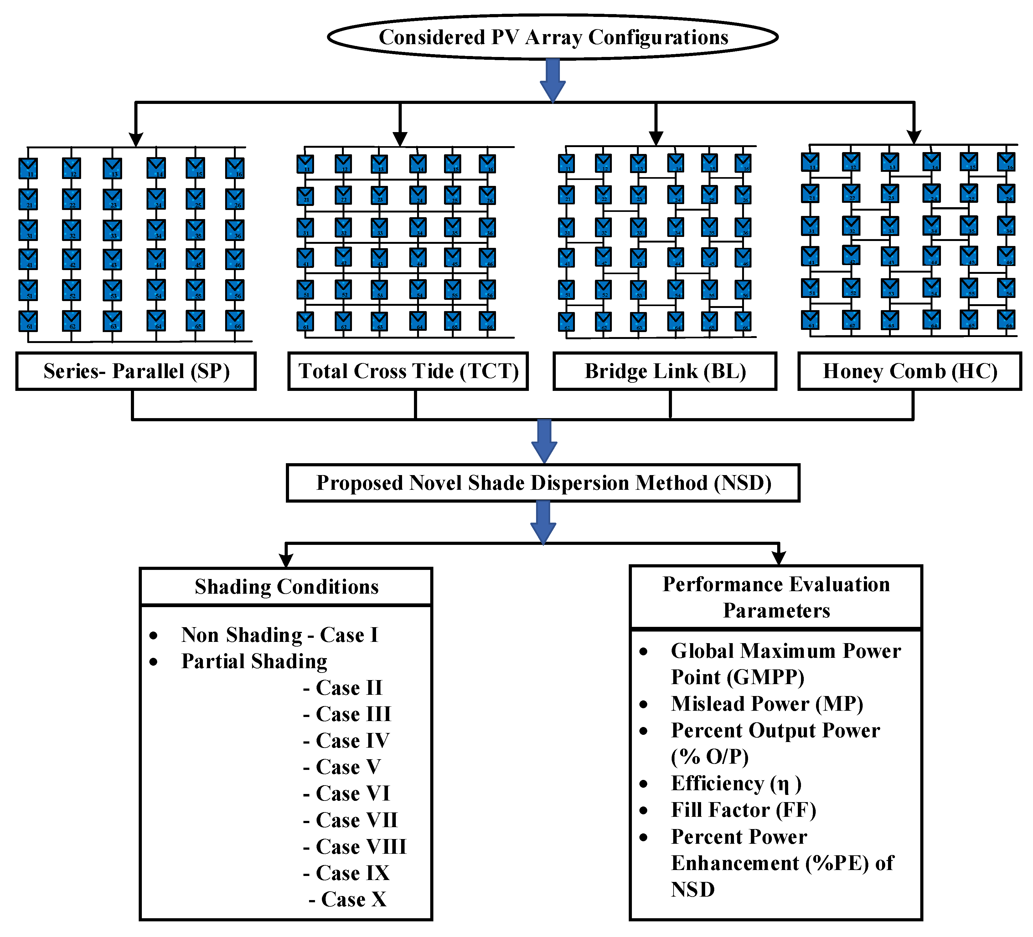
• The proposed scheme was analyzed under ten shading cases. The results validated with SP, TCT, BL, and HC compared the global maximum power point (GMPP), mislead power (MP), output power (%O/P), efficiency, fill factor, and % power enhancement for NSD under-considered shading pattern. Figure 1 gives the workflow of this paper.

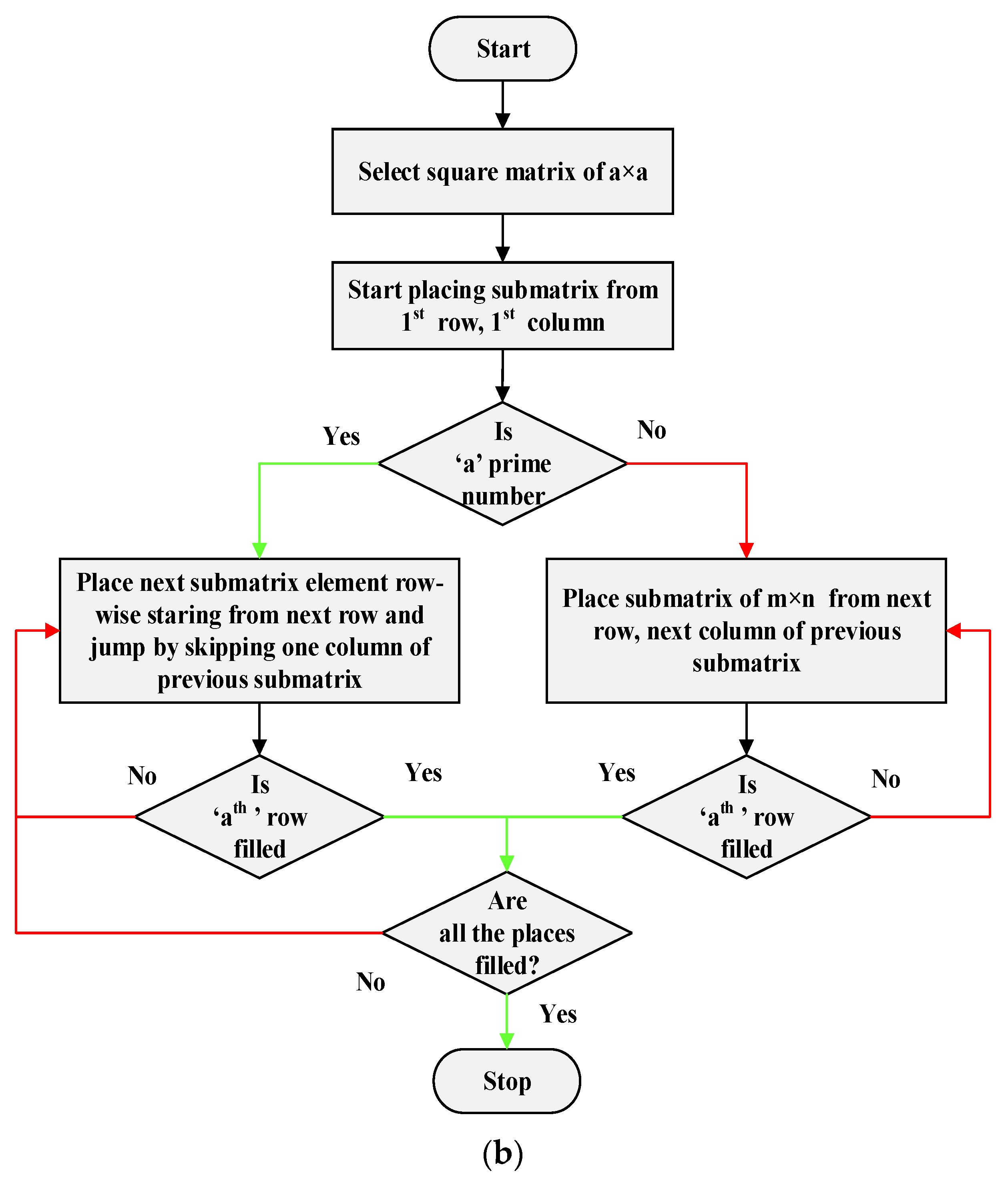
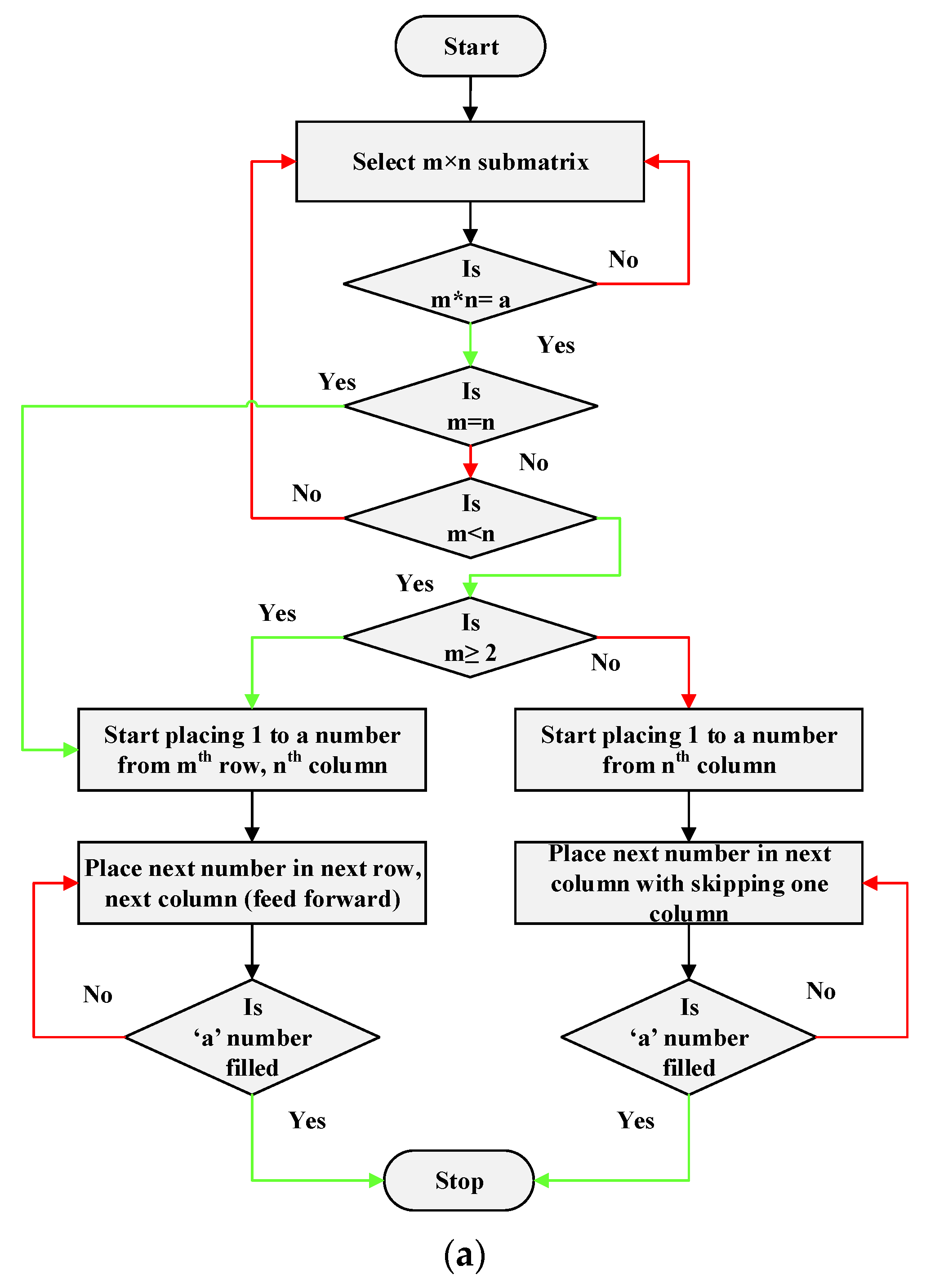
2. Modeling and Simulation of NSD Method

This section explains the modeling and simulation of conventional PV array configurations and the proposed novel shade dispersion (NSD) method in MATLAB/Simulink. The panel electrical parameters has mentioned in Appendix A. The flowchart for panel repositioning is provided in Figure 2. The present work consists of 36 modules placed in six rows and six column patterns (shown in Figure 3a) for conventional configurations and the NSD method (Figure 3b). The TCT connection-based MATLAB simulation is shown in Figure 4. Mathematical modeling for output voltage, output current, and output power of all the traditional PV array structures are provided in

Table 1. The output voltage, current, and power for conventional PV array configurations.

Connection	Output Voltage	Output Current	Output Power
SP	${\mathrm{V}}_{\mathrm{PV}}={\displaystyle {\displaystyle \sum }_{\mathrm{j}=1}^6}{\mathrm{V}}_{\mathrm{j}}=6{\mathrm{V}}_{\mathrm{j}}$	${\mathrm{I}}_{\mathrm{PV}}={\displaystyle {\displaystyle \sum }_{\mathrm{j}=1}^6}{\mathrm{I}}_{\mathrm{Sj}}=6{\mathrm{I}}_{\mathrm{S}}$	${\mathrm{P}}_{\mathrm{PV}}=36{\mathrm{V}}_{\mathrm{j}}{\mathrm{I}}_{\mathrm{S}}$
TCT	${\mathrm{V}}_{\mathrm{PV}}={\displaystyle {\displaystyle \sum }_{\mathrm{j}=1}^6}{\mathrm{V}}_{\mathrm{j}}=6{\mathrm{V}}_{\mathrm{j}}$	${\mathrm{I}}_{\mathrm{PV}}={\mathrm{I}}_1+{\mathrm{I}}_7+{\mathrm{I}}_{13}+{\mathrm{I}}_{17}+{\mathrm{I}}_{23}+{\mathrm{I}}_{29}=6{\mathrm{I}}_{\mathrm{S}}$	${\mathrm{P}}_{\mathrm{PV}}=36{\mathrm{V}}_{\mathrm{j}}{\mathrm{I}}_{\mathrm{S}}$
BL	${\mathrm{V}}_{\mathrm{PV}}={\displaystyle {\displaystyle \sum }_{\mathrm{j}=1}^6}{\mathrm{V}}_{\mathrm{j}}=6{\mathrm{V}}_{\mathrm{j}}$	${\mathrm{I}}_{\mathrm{PV}}={\mathrm{I}}_{\mathrm{S}1}+{\mathrm{I}}_{\mathrm{S}2}+{\mathrm{I}}_{\mathrm{S}3}+{\mathrm{I}}_{\mathrm{S}4}+{\mathrm{I}}_{\mathrm{S}5}+{\mathrm{I}}_{\mathrm{S}6}=6{\mathrm{I}}_{\mathrm{S}}$	${\mathrm{P}}_{\mathrm{PV}}=36{\mathrm{V}}_{\mathrm{j}}{\mathrm{I}}_{\mathrm{S}}$
HC	${\mathrm{V}}_{\mathrm{PV}}={\displaystyle {\displaystyle \sum }_{\mathrm{j}=1}^6}{\mathrm{V}}_{\mathrm{j}}=6{\mathrm{V}}_{\mathrm{j}}$	${\mathrm{I}}_{\mathrm{PV}}={\mathrm{I}}_{\mathrm{S}1}+{\mathrm{I}}_{\mathrm{S}2}+{\mathrm{I}}_{\mathrm{S}3}+{\mathrm{I}}_{\mathrm{S}4}+{\mathrm{I}}_{\mathrm{S}5}+{\mathrm{I}}_{\mathrm{S}6}=6{\mathrm{I}}_{\mathrm{S}}$	${\mathrm{P}}_{\mathrm{PV}}=36{\mathrm{V}}_{\mathrm{j}}{\mathrm{I}}_{\mathrm{S}}$

. Here, the module, row, and array output voltages are ${\mathrm{V}}_{\mathrm{j}}$, ${\mathrm{V}}_{\mathrm{R}}$, and ${\mathrm{V}}_{\mathrm{PV}}$, respectively. The module, string, and array output currents are ${\mathrm{I}}_{\mathrm{j}}$, ${\mathrm{I}}_{\mathrm{S}}$, and ${\mathrm{I}}_{\mathrm{PV}}$. ${\mathrm{P}}_{\mathrm{PV}}$ is the PV generation of the array. A novel shade dispersion method is proposed to reconfigure the panel of a variety to improve the performance through shade dispersion. In the proposed technique, electrical connections remain the same as in TCT [20]; only the physical location of the modules changes. It uses voltage, current, and power equations for TCT, as mentioned in Table 1. The basic principle used for this method is row current equalization. It proposes a magic submatrix arrangement with the magic number 21 and its logical shifting to reposition the panels within a column, as shown in Figure 3b.

The steps involved to build the proposed 6 × 6 NSD matrix are:

Step I: Formation of the submatrix

• The submatrix is proposed so that rows and column multiplication of the submatrix is 6;
• Therefore, numbers 1 to 6 are placed in the 2 × 3 submatrix to summation equal to the magic number 21;

Step II: Formation of the primary matrix

3.

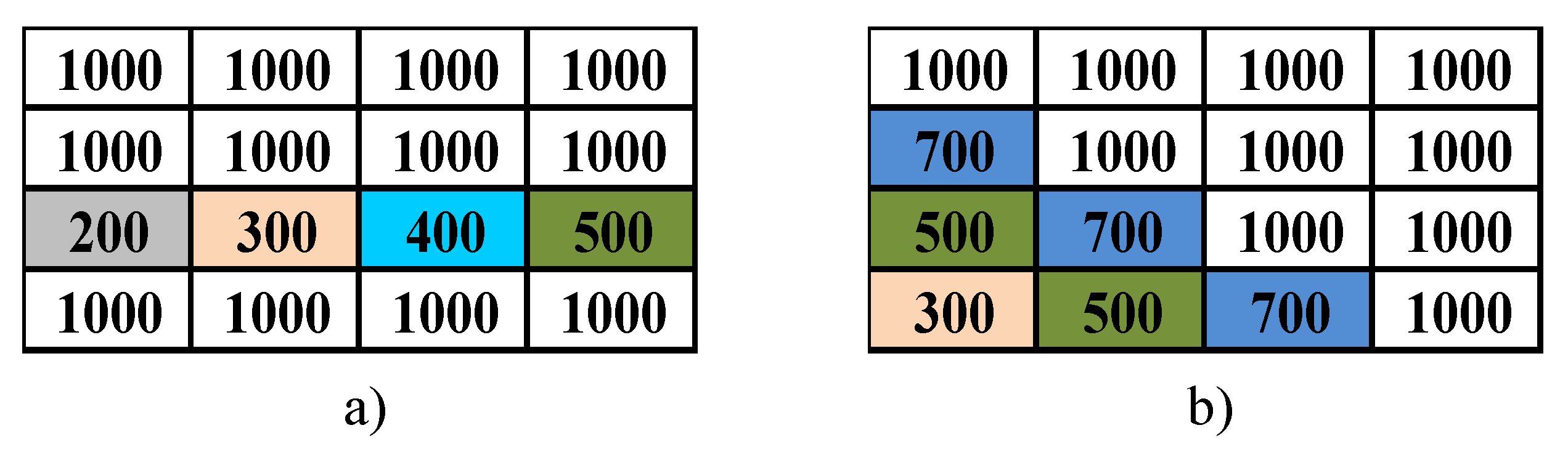
The submatrix placing is started in the 1st row, 1st column position. The next submatrix is placed at the next (3rd) row, next (2nd) column position. This process continues until the last (6th) row is filled by the considered submatrix;

4.

Submatrix rows are interchanged, and that submatrix starts to fill in vacant places of the primary matrix, starting from the next column of previously filled areas. Here, the interchanged submatrix is filled from 1st row, 4th column. The next submatrix is placed in the 3rd row and 4th column. The last column of the submatrix is placed in the same row and vacant column serially;

5.

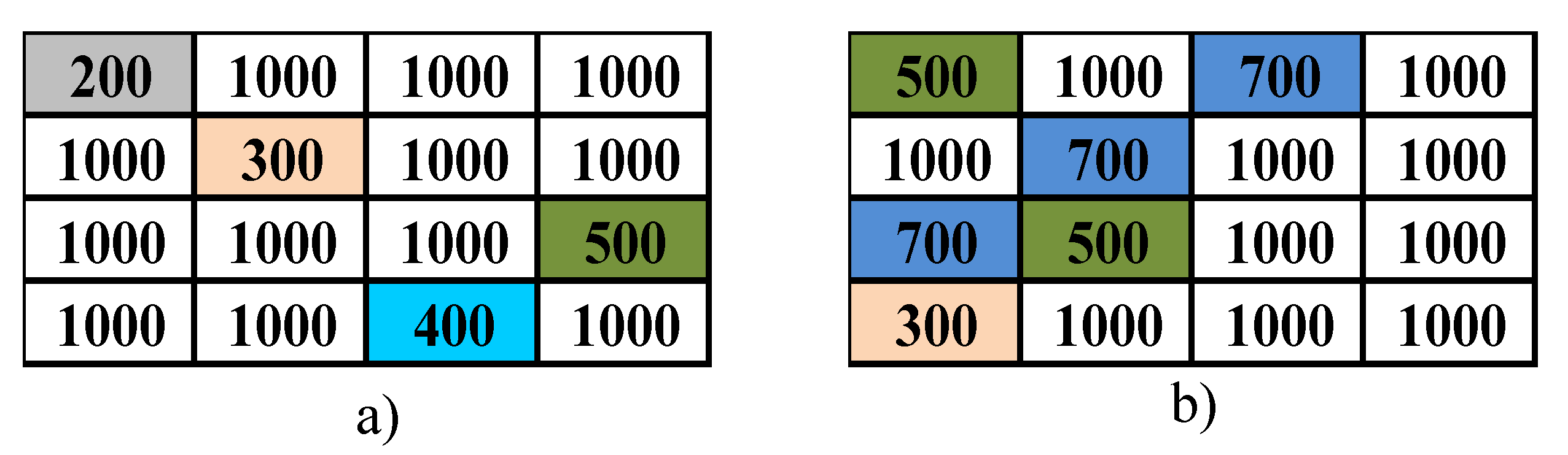
It is performed so that the summation of row numbers, as well as column numbers, is equal to the magic number 21, as shown in Figure 3b;

6.

The process continues until vacant places in the primary matrix are filled, and the fifth step is achieved.

3. Partial Shadings Conditions and Shade Dispersion Effect

For CCs the shade does not scatter, as shown in Figure 5. Through NSD, the partial shading condition spread on a complete array, as shown in Figure 6. Under case I (i.e., non-shading condition), the performance of the NSD method is the same as the CC (i.e., without reconfiguration), as shown in Figure 7a. The performance indicators are the global maximum power point (GMPP), mislead nine PSCs as power (MP), output power (%O/P), efficiency, fill factor, and % power enhancement of NSD. The %PE was calculated for NSD and compared with all the CCs. For case I, all 36 modules of the PV array have 1000 W irradiance; the remaining PSCs have four groups of irradiance.

• Case II to case IV have group 1 of 24 panels with 1000 W irradiance; groups 2, 3, and 4 have 200 W, 500 W, and 700 W irradiance, respectively, with four panels in each group;
• In case V, 10 modules have PSCs, group 1 with 1000 W has 26 panels. Group 2, with 200 W, has four modules, and groups 3 and 4 have 500 W, 700 W irradiance, respectively, with three panels;
• Case VI has groups 1, 2, 3, and 4 with 1000 W, 200 W, 500 W, and 700 W irradiance on 28, 3, 1, and 4 modules, respectively;
• In case VII, 24 panels came in group 1. Groups 2 and 3, have 200 W and 700 W irradiance, respectively. Group 4 has two panels that have 700 W irradiance;
• In case VIII, groups 1, 2, 3, and 4 have five panels in each group of 1000 W, 200 W, 500 W, and 700 W irradiance with 16, 8, 7, and five panels, respectively;
• In case IX, only five modules are partially shaded, and 31 modules have 1000 W irradiance in group 1. It has two 200 W modules in group 2, one 500 W module in group 3 and two 700 W irradiance panels in group 4;
• In case X, with 1000 W, group 1 has 25 panels. Group 2, with 200 W has four panels, and groups 3 and 4 have 500 W and 700 W irradiance, respectively, with three panels.

4. Result and Discussion

The performance evaluation of PV array CCs and proposed reconfiguration was performed under various shading situations on MATLAB/Simulink. The assessment has two segments, (1) power-voltage profile and (2) computational parameters.

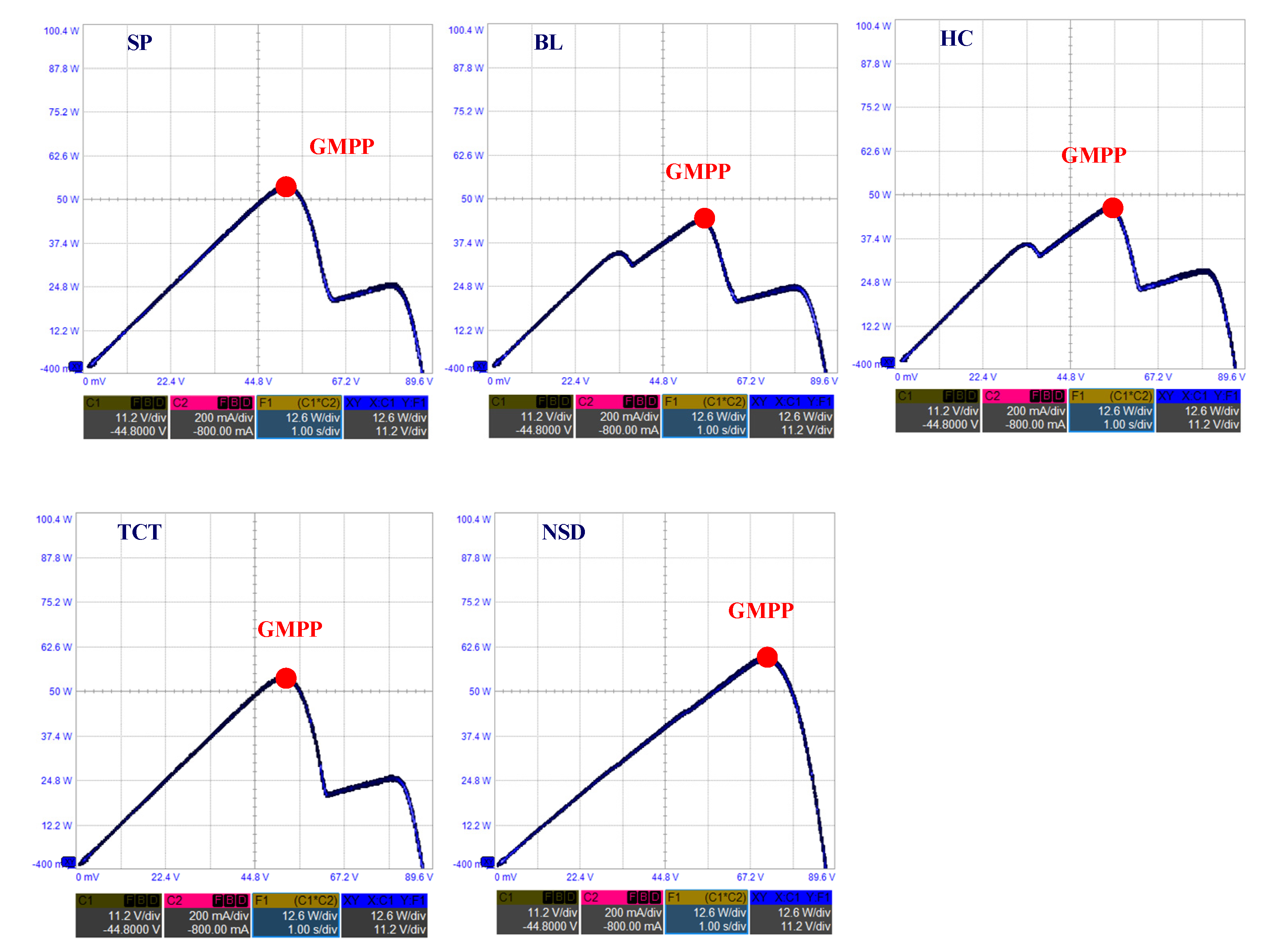
4.1. Power-Voltage Profiles under Various PSC

The sketches in Figure 7 represent the variation in PV curves for different conventional configurations and the proposed NSD method of reconfiguration under various irradiance levels. Under case I of the non-shading condition, all the panels have the same standard irradiance of 1000 W. Figure 7a highlights that all the configuration and NSD methods have the same ideal performance under case I with only one peak on the PV curve.

Under case II, conventional configurations have two peaks on the PV curve, while the NSD method has only one extreme. TCT, BL, and HC have identical extreme power, and it is more than SP, while for NSD, the maximum capacity is much more enhanced, as revealed in Figure 7b. Figure 7c indicates that SP has the lowest power output for case III. It offers continuous improvement for BL, HC, TCT, and NSD. NSD offers 6234 W as the maximum power output. In Figure 7d, SP has three peaks, and other methods have two heights. BL and HC show improved performance over SP but lesser than TCT and NSD. NSD provides the highest output of 6234 W, as shown. Figure 7e portrays that BL and HC have six peaks, SP and TCT have five peaks, while NSD is reduced to four peaks and the highest power generation equal to 6303 W for case V. In Figure 7f case VI, HC and SP have the same maximum power generation as BL and TCT with three peaks; in contrast, the NSD has the highest power generation of 6646 W with three small deep peaks. Figure 7g showcases the case VII PV curves for SP, TCT, BL, HC, and NSD. NSD has a single top with 6133 W as the highest power generation. In Figure 7h SP and TCT have six and four peaks. BL, HC, and NSD structures have three peaks with the highest power, 5160 W, for the NSD method. Figure 7i portrays case IX. Under this shade, TCT has maximum power extraction of 6563 W in conventional configuration while NSD has improved power extraction with 6953 W.

4.2. Computational Parameters

The performances of all CC and NSD were investigated in the following six computational parameters, as observed in Appendix B, which highlights the efficacy of NSD over CC.

Table 2. SP performance under PSC.

Shade Cases	VOC (V)	ISC (A)	No. of Peaks	PM (W)	VM (V)	IM (A)
Case I	217.80	47.16	1	7665.80	174.00	44.00
Case II	217.80	43.49	2	4654.30	115.15	40.42
Case III	217.80	38.64	2	5655.20	174.98	32.31
Case IV	217.80	47.15	4	4711.90	115.76	44.00
Case V	217.80	45.23	5	5005.40	160.34	31.21
Case VI	216.31	44.81	3	5818.10	153.06	38.01
Case VII	214.91	43.49	4	4496.00	123.36	36.45
Case VIII	213.54	37.49	6	3309.10	115.42	28.67
Case IX	216.81	47.16	4	6068.50	175.65	34.55
Case X	215.89	44.80	5	5768.50	164.53	35.06

,

Table 3. TCT performance under PSC.

Shade Cases	VOC (V)	ISC (A)	No. of Peaks	PM (W)	VM (V)	IM (A)
Case I	217.70	47.16	1	7665.80	174.00	44.00
Case II	215.41	47.16	2	5039.80	114.48	44.02
Case III	215.76	42.42	3	6001.20	179.43	33.45
Case IV	215.90	44.74	4	6028.20	180.12	33.47
Case V	215.30	47.14	5	4627.30	189.10	27.74
Case VI	216.48	44.80	3	5833.80	147.02	39.68
Case VII	215.09	47.15	4	4807.50	116.94	41.11
Case VIII	214.02	42.44	4	4172.10	118.73	35.14
Case IX	216.95	47.15	3	6563.30	181.91	36.08
Case X	216.01	44.78	4	6093.50	180.53	33.75

,

Table 4. BL performance under PSC.

Shade Cases	VOC (V)	ISC (A)	No. of Peaks	PM (W)	VM (V)	IM (A)
Case I	217.00	47.16	1	7665.80	174.00	44.05
Case II	215.36	47.16	2	5039.80	114.48	44.02
Case III	215.73	42.43	3	5849.50	178.21	32.82
Case IV	216.03	44.79	3	5749.20	146.56	41.22
Case V	216.30	47.15	6	5036.20	184.84	27.24
Case VI	216.40	44.80	3	5706.00	148.28	38.48
Case VII	215.01	47.15	4	4702.90	117.56	40.00
Case VIII	213.57	39.29	3	4033.20	115.99	34.77
Case IX	216.90	47.15	4	6300.60	179.86	35.03
Case X	215.97	44.79	3	5862.10	178.79	32.79

,

Table 5. HC performance under PSC.

Shade Cases	VOC (V)	ISC (A)	No. of Peaks	PM (W)	VM (V)	IM (A)
Case I	217.78	47.16	1	7665.80	174.00	44.00
Case II	215.33	47.16	2	5039.80	114.48	44.00
Case III	215.75	42.43	4	5913.70	179.34	32.97
Case IV	215.63	44.79	2	5674.10	146.28	38.78
Case V	216.40	47.15	6	5102.40	185.66	27.48
Case VI	216.38	44.81	3	5873.30	151.80	38.69
Case VII	214.98	47.16	4	4797.10	119.08	40.29
Case VIII	213.59	39.30	3	4042.00	116.37	34.74
Case IX	216.90	47.16	2	6320.40	179.78	35.16
Case X	216.04	47.14	5	5915.20	179.48	32.96

and

Table 6. NSD performance under PSC.

Shade Cases	VOC (V)	ISC (A)	No. of Peaks	PM (W)	VM (V)	IM (A)
Case I	217.79	47.17	1	7665.80	174.00	44.06
Case II	215.79	40.86	1	6234.00	175.95	35.43
Case III	215.79	40.86	1	6234.00	175.95	35.43
Case IV	215.94	44.75	3	6211.00	177.56	34.98
Case V	216.04	44.75	4	6303.20	177.23	35.56
Case VI	216.54	44.78	3	6645.70	177.48	37.44
Case VII	215.54	39.25	1	6132.90	174.90	35.07
Case VIII	213.98	34.57	3	5160.20	176.34	29.26
Case IX	216.97	47.10	2	6952.80	176.76	39.34
Case X	216.04	43.18	2	6350.60	177.09	35.86

give the performance of SP, TCT, BL, HC and NSD method under ten PSCs respectively.

4.2.1. Global Maximum Power Point (GMPP)

The PV curve has multiple peaks due to PSC, as shown in Figure 8. GMPP is the maximum power of all the crests. Figure 8a indicates that GMPP for all CCs and NSD have concentrated 7665 W. For case II, TCT, BL, and HC provide equal power at 5039 W in CC, and NSD improves it up to 6234 W. Case III also NSD has GMPP at 6234 W. Under case IV in CC, TCT provides maximum output at 6028 W while NSD has 6211 W. Under case V, NSD has 6303 W as a GMPP; this is 1201 W more than HC, which offers the highest power of all CCs. Under case VI to case X in CC, TCT offers the uppermost GMPP while NSD has GMPP at 6646 W, 6133 W, 5160 W, 6953 W, and 6350 W for respective PSC. It is 812 W, 1325 W, 988 W, 389 W, and 257 W more than TCT under the same PSCs.

4.2.2. Mislead Power (MP)

Figure 8b shows that the proposed NSD method provides the least misleading power as the red NSD trace is at the innermost on the radar pattern. Case I does not have any MP. From case II to case X it is 1431 W, 1431.8 W, 1454 W, 1363 W, 1020 W, 1533 W, 2506 W, 713 W, and 1315 W continuously. NSD reduces the MP by about 11 to 46% under these shading cases.

4.2.3. Percent Output (%O/P)

Figure 8c Highlights that all considered structure provides 100% output for case I. NSD provides 81% O/P, the maximum from cases II, III, and IV. In CC, HC provides the highest %O/P at 66.5% under case V, while NSD improves it to 82.69%. In CC under case VI to case X, TCT offers the uppermost %O/P, and NSD improved it by 10.5%, 17.3%, 12.9%, 5%, and 3.4% compared with TCT for the respective shading cases.

4.2.4. Efficiency (η)⁻

Figure 8d shows the NSD structure is more efficient than TCT, which has the same electrical connections; under-considered PSCs. The radar pattern representation in Figure 8d clearly shows that NSD offers efficiency near 21%. It is approximately equal to the PV array efficiency for case I.

4.2.5. Fill Factor (FF)⁻

Figure 8e highlights that the proposed method offers 2–5% improvement in FF for cases III, IV, IX, and X; 15.19% more FF for case V, 8% improvement for case VI, and 20–25% enhancement for case II, VII, and VIII, compared with maximum FFs in CC.

4.2.6. Percent Power Enhancement (%PE)

The %PE ensures the power increment by the proposed reconfiguration. Figure 8f shows that NSD improves power extraction compared with CC. Compared with SP, TCT, BL, and HC, NSD has a 25.9, 15.79, 17.44, and 16.45% power boost.

Figure 8. Performance evaluation parameter (a) GMPP (W), (b) MP(W), (c)%O/P, (d) η, (e) FF, (f) %PE.

Figure 8. Performance evaluation parameter (a) GMPP (W), (b) MP(W), (c)%O/P, (d) η, (e) FF, (f) %PE.

5. Experimental Implementation and Result Analysis

5.1. Experimental Setup

Towards real-time implementation of the proposed NSD method, a prototype laboratory experiment with 16 PV modules and a 4 × 4 array structure was conducted on the PV chroma 62050 H-600 S simulator (Taiwan). The chroma 63203 E DC (Taiwan) electronic load was used to develop an experimental setup, as shown in Figure 9. The electrical parameters for each 5 Watt panel are, V_OC = 21.6 V, V_M = 17.5 V, I_SC = 0.3 A, I_M = 0.29 V. Under non-shading conditions, this PV array provides 80 W power generation.

As shown in Figure 10 and Figure 11, two types of irradiance circumstances were examined in the experiment. The shading patterns considered for experimentation were horizontal (case I) and triangular corner (case II). These are similar to case II and case V in Section 2 but with different irradiance levels and array sizes. The shade concentrates before reconfiguring this array structure, as shown in Figure 10, for all the conventional configurations. After applying the proposed NSD reconfiguration, the shadow was distributed on the array, as shown in Figure 11.

5.2. Experimental Result Analysis

To perform the analysis of conventional configurations, SP, BL, HC, TCT, and the proposed NSD reconfiguration, the PV curve nature was obtained by changing the load resistance through DC Electronic load from 4000 Ω to 1 Ω. The curve nature was observed on an HDO4034A (USA) 350 MHz high-definition oscilloscope.

5.2.1. PSC Case I

Figure 12 depicts the PV curves for each conventional configuration, NSD reconfiguration scheme, and the global MPP (the dot on the PV curve) under PSC case I. The PV curve shows GMPP for SP, BL, HC, TCT, and NSD at 59.22 W, 49.79 W, 49.79 W, 59.23 W, and 66.57 W, respectively. Moreover, SP and TCT have two peaks on the PV curve, BL and HC have three heights, and NSD reconfiguration reduces the number of peaks.

5.2.2. PSC Case II

Under this shading condition, Figure 13 shows that all conventional configurations have three peak PV curves. In contrast, the proposed NSD reconfiguration has one minor local peak and GMPP at a higher level with an improved curve nature. SP, BL, HC, TCT, and NSD provide GMPP at 52.92 W, 54.63 W, 53.75 W, 56.04 W, and 70.03 W, respectively. Figure 13 highlights that there is much improvement in the PV curve nature under this shading condition and GMPP location.

6. Conclusions

From the discussion mentioned above, this study concludes that:

• In partial shading cases, for the least irradiating case VIII and most irradiating case IX, NSD has maximum power extraction of 5160 W and 6952.8 W, respectively; the highest efficiency of 20.97% and 20.87%, respectively; FF is 0.6976 and 0.6803, respectively; and the lowest ML of 2505.6 W and 713 W among all configurations, respectively;
• Under PSC for the considered PV array, TCT has the highest GMPP, %O/P, efficiency, FF, %PE, and least %MP at 5683 W, 74%, 18.54%, 0.5784, and 28.73%. Compared with TCT, NSD has 705.77 W, 9.2%, and 0.1139 enhancement in GMPP, %O/P, and FF, and a 2.41% reduction in MP;
• The results obtained from the first simulation show that the NSD method achieved the most significant output power and overall performance compared with all conventional configurations under nine partial shading cases;
• Moreover, experimental research was carried out. The suggested NSD PV array reconfiguration design beats the other conventional PV array configurations (SP, BL, HC, and TCT) in power increase and several peaks. The experimental setup validated the influence of panel shifting on various PV array topologies.

References

- Sahoo, S.K. Renewable and sustainable energy reviews solar photovoltaic energy progress in India: A review. Renew. Sustain. Energy Rev. 2016, 59, 927–939. [Google Scholar] [CrossRef]
- Fouad, M.M.; Shihata, L.A.; Morgan, E.S.I. An integrated review of factors influencing the performance of photovoltaic panels. Renew. Sustain. Energy Rev. 2017, 80, 1499–1511. [Google Scholar] [CrossRef]
- Venkateswari, R.; Sreejith, S. Factors influencing the efficiency of photovoltaic system. Renew. Sustain. Energy Rev. 2019, 101, 376–394. [Google Scholar] [CrossRef]
- Attivissimo, F.; Di Nisio, A.; Savino, M.; Spadavecchia, M. Uncertainty analysis in photovoltaic cell parameter estimation. IEEE Trans. Instrum. Meas. 2012, 61, 1334–1342. [Google Scholar] [CrossRef]
- Hysa, A. Modeling and Simulation of the Photovoltaic Cells for Different Values of Physical and Environmental Parameters. Emerg. Sci. J. 2019, 3, 395–406. [Google Scholar] [CrossRef] [Green Version]
- Praveen Kumar, B.; Prince Winston, D.; Cynthia Christabel, S.; Venkatanarayanan, S. Implementation of a switched PV technique for rooftop 2 kW solar PV to enhance power during unavoidable partial shading conditions. J. Power Electron. 2017, 17, 1600–1610. [Google Scholar] [CrossRef]
- Ziar, H.; Nouri, M.; Asaei, B.; Farhangi, S. Analysis of overcurrent occurrence in photovoltaic modules with overlapped by-pass diodes at partial shading. IEEE J. Photovolt. 2014, 4, 713–721. [Google Scholar] [CrossRef]
- Mäki, A.; Valkealahti, S. Power losses in long string and parallel-connected short strings of series-connected silicon-based photovoltaic modules due to partial shading conditions. IEEE Trans. Energy Convers. 2012, 27, 173–183. [Google Scholar] [CrossRef]
- Hussan, R.; Sarwar, A. Maximum power point tracking techniques under partial shading condition-A review. In Proceedings of the 2018 2nd IEEE International Conference on Power Electronics, Intelligent Control and Energy Systems, New Delhi, India, 22–24 October 2018; pp. 293–298. [Google Scholar] [CrossRef]
- Bana, S.; Saini, R.P. Experimental investigation on power output of different photovoltaic array configurations under uniform and partial shading scenarios. Energy 2017, 127, 438–453. [Google Scholar] [CrossRef]
- Pendem, S.R.; Mikkili, S. Modelling and performance assessment of PV array topologies under partial shading conditions to mitigate the mismatching power losses. Sol. Energy 2018, 160, 303–321. [Google Scholar] [CrossRef]
- Bingöl, O.; Özkaya, B. Analysis and comparison of di ff erent PV array con fi gurations under partial shading conditions. Sol. Energy 2018, 160, 336–343. [Google Scholar] [CrossRef]
- Raju, V.B.; Chengaiah, C. Power Enhancement of Solar PV Arrays under Partial Shading Conditions with Reconfiguration Methods. In Proceedings of the 2019 Innovations in Power and Advanced Computing Technologies (i-PACT), Vellore, India, 22–23 March 2019; pp. 1–7. [Google Scholar] [CrossRef]
- Ajmal, A.M.; Sudhakar Babu, T.; Ramachandaramurthy, V.K.; Yousri, D.; Ekanayake, J.B. Static and dynamic reconfiguration approaches for mitigation of partial shading influence in photovoltaic arrays. Sustain. Energy Technol. Assess. 2020, 40, 100738. [Google Scholar] [CrossRef]
- Manjunath, M.; Reddy, B.V.; Lehman, B. Performance improvement of dynamic PV array under partial shade conditions using M2 algorithm. IET Renew. Power Gener. 2019, 13, 1239–1249. [Google Scholar] [CrossRef]
- Varma Gadiraju, H.K.; Reddy Barry, V.; Maraka, I. Dynamic Photovoltaic Array Reconfiguration for Standalone PV Water Pumping System. In Proceedings of the 2019 8th International Conference on Power Systems: Transition towards Sustainable, Smart and Flexible Grids (ICPS), Jaipur, India, 20–22 December 2019; IEEE: Piscataway, NJ, USA, 2019; pp. 29–32. [Google Scholar] [CrossRef]
- Bularka, S.; Gontean, A. Dynamic PV array reconfiguration under suboptimal conditions in hybrid solar energy harvesting systems. In Proceedings of the 2017 IEEE 23rd International Symposium for Design and Technology in Electronic Packaging, Constanta, Romania, 26–29 October 2017; pp. 419–422. [Google Scholar] [CrossRef]
- Pachauri, R.K.; Alhelou, H.H.; Bai, J.; Golshan, M.E.H. Adaptive Switch Matrix for PV Module Connections to Avoid Permanent Cross-Tied Link in PV Array System under Non-Uniform Irradiations. IEEE Access 2021, 9, 45978–45992. [Google Scholar] [CrossRef]
- Rani, B.I.; Ilango, G.S.; Nagamani, C. Enhanced power generation from PV array under partial shading conditions by shade dispersion using Su Do Ku configuration. IEEE Trans. Sustain. Energy 2013, 4, 594–601. [Google Scholar] [CrossRef]
- Sai Krishna, G.; Moger, T. Improved SuDoKu reconfiguration technique for total-cross-tied PV array to enhance maximum power under partial shading conditions. Renew. Sustain. Energy Rev. 2019, 109, 333–348. [Google Scholar] [CrossRef]
- Sreekantha Reddy, S.; Yammani, C. A novel Magic-Square puzzle based one-time PV reconfiguration technique to mitigate mismatch power loss under various partial shading conditions. Optik 2020, 222, 165289. [Google Scholar] [CrossRef]
- Vijayalekshmy, S.; Bindu, G.R.; Rama Iyer, S. Performance comparison of Zig-Zag and Su do Ku schemes in a partially shaded photo voltaic array under static shadow conditions. In Proceedings of the 2017 Innovations in Power and Advanced Computing Technologies (i-PACT), Vellore, India, 21–22 April 2017; pp. 1–6. [Google Scholar] [CrossRef]
- Dhanalakshmi, B.; Rajasekar, N. A novel Competence Square based PV array reconfiguration technique for solar PV maximum power extraction. Energy Convers. Manag. 2018, 174, 897–912. [Google Scholar] [CrossRef]
- Nihanth, M.S.S.; Ram, J.P.; Pillai, D.S.; Ghias, A.M.Y.M.; Garg, A.; Rajasekar, N. Enhanced power production in PV arrays using a new skyscraper puzzle based one-time reconfiguration procedure under partial shade conditions (PSCs). Sol. Energy 2019, 194, 209–224. [Google Scholar] [CrossRef]