Abstract
Accurate state of charge (SOC) plays a vital role in battery management systems (BMSs). Among several developed SOC estimation methods, the extended Kalman filter (EKF) has been extensively applied. However, EKF cannot achieve valid estimation when the model accuracy is inadequate, the noise covariance matrix is uncertain, and the sensor has large errors. This paper makes two contributions to overcome these drawbacks: (1) A variable forgetting factor recursive least squares (VFFRLS) is proposed to accomplish parameters identification. This method updates the forgetting factor according to the innovation sequence, which accuracy is superior to the forgetting factor recursive least squares (FFRLS); (2) an adaptive tracking EKF (ATEKF) is proposed to estimate the SOC of the battery. In ATEKF, the error covariance matrix is adaptively corrected according to the innovation sequence and correction factor. The value of the correction factor is related to the actual error. Proposed algorithms are validated with a publicly available dataset from the University of Maryland. The experimental results indicate that the identification error of VFFRLS can be reduced from 0.05% to 0.018%. Additionally, ATEKF has better accuracy and robustness than EKF when having large sensor errors and uncertainty of the error covariance matrix, in which case it can reduce SOC estimation error from 1.09% to 0.15%.
1. Introduction
With the increasing environmental pollution, governments are giving increasing attention to the problem of pollution caused by energy. Meanwhile, electric vehicles (EVs) have become a crucial development in the automotive industry [1,2,3]. Lithium-ion batteries (LIBs) have the advantages of low weight, low self-discharge rate, high energy density, and high power density [4]. Therefore, LIBs are widely applied in EVs. However, LIBs in EVs are often operated in a very complex environment, and their dynamic behavior is strongly nonlinear. If the BMS cannot accurately estimate the SOC, possible overcharge and discharge current can cause irreversible damage to the capability and lifetime of LIBs [5,6].
At present, numerous battery SOC estimation methods have been proposed, with some advantages and disadvantages [7,8]. The most popular LIBs SOC estimation methods are as follows: open-circuit voltage method, ampere-hour counting method, data-driven method, and model-based method. The open-circuit voltage method needs LIBs to be stationary for a long time. Obviously, this method is not applicable to driving EVs. It is merely suitable for environments such as a laboratory. The ampere-hour counting method is the most commonly used method, which is elementary to implement. However, its accuracy is affected by LIB capacity, initial SOC of LIBs, and current sensor error. These disadvantages lead ampere-hour counting method being easy to accumulate errors with large current fluctuations [9]. The data-based method eliminates the system modeling, which only requires the input and output data to train the model for SOC estimation. However, this method needs to collect a massive volume of data, and the performance of the model is greatly determined by the quality of data [10,11,12]. The model-based approaches can be divided into three categories depending on the model. Among them, the Kalman filter (KF), based on the equivalent circuit model (ECM), is the most classical. As KF has good accuracy and acceptable computational volume, it can be widely applied to practical applications.
In recent years, KF and its derivative algorithms are extremely popular in the field of LIB SOC estimation. The estimation principle of KF is a recursive minimum method, which can achieve a dynamic estimation of the system state. KF is very suitable for the SOC estimation of EV batteries because it provides a reasonable balance between complexity and accuracy. Meanwhile, there are some limitations to KF [13,14,15]. Since KF is a SOC estimation method based on ECM, the accuracy of ECM influences SOC estimation. Therefore, it is essential to enhance the accuracy of ECM while ensuring the computational power of the algorithm. References [16,17] proposed a parameter identification algorithm based on FFRLS, which can set forgetting factors to adjust the weights of new data. However, the forgetting factor of this algorithm is set to be a constant throughout the identification process, and the accuracy of identified model parameters is not high under complex driving conditions. Reference [18] proposed a simulated annealing optimized particle swarm optimization (SA-PSO), which has excellent local searchability. However, it cannot online identify the parameters of ECM, so it is not applicable to LIBs in EVs. Reference [19] proposed an adaptive Kalman filter (AEKF) estimation method based on a fractional order model. Despite this method having high estimation accuracy, the identification of model parameters is complicated. Reference [20] proposed a combination algorithm of AUKF and STUKF, which has strong tracking capability and accuracy. However, the model uncertainty threshold for fusing the two algorithms needs to be derived by the trial patch method. Reference [21] proposed a particle swarm and extended Kalman filter fusion algorithm (PSO-EKF), which has better convergence and robustness. However, PSO as a global optimization algorithm requires a large amount of computation. Reference [22] proposed a fusion algorithm of ampere-hour counting and extended Kalman filter (EKF-AH). This method has wonderful robustness to sensor error, but when the sensor errors are slight, the proposed algorithm is rather less effective than EKF.
Considering the LIBs of EVs working in a complex environment, in this paper, two algorithms are proposed, which can accurately estimate the SOC in the case of large sensor errors and uncertainty in the error covariance [23]. After testing in some dynamic operating conditions, the algorithms can adapt to the practical requirements of EVs. To reduce the error of ECM, a variable forgetting factor recursive least squares (VFFRLS) method is proposed in this paper, which can adaptively update the forgetting factor according to the innovation sequence. Additionally, in order to improve the accuracy and robustness of SOC estimation, we propose an adaptive tracking-extend Kalman filter (ATEKF) algorithm. The experiments confirm that ATEKF has better accuracy and robustness than EKF and AEKF. This means that the ATEKF can operate in more complex environments, such as battery aging and battery thermal models [5].
The primary contributions of this paper are as follows:
- A VFFRLS method is proposed, which can adaptively update the forgetting factor. Compared with the FFRLS algorithm, this method can improve the accuracy of identified parameters;
- An ATEKF method is proposed to accomplish the SOC estimation of EVs. The experiments show that ATEKF has better accuracy than EKF and AEKF;
- Under voltage drift and uncertain error covariance, the ATEKF has better robustness and lower error. It is more suitable for the SOC estimation of EVs.
The rest of this paper is organized as follows: In Section 2, the ECM and parameter identification methods of ECM are discussed; in Section 3, the SOC estimation method based on ATEKF is introduced; the battery experimental dataset utilized for validation is presented in Section 4, followed by the verification of the performance of VFFRLS and ATEKF in Section 5; lastly, conclusions of this paper are presented in Section 6.
2. Battery Modeling
2.1. Equivalent Circuit Models and Parameter Identification
At present, LIB models can be divided into three types—namely, equivalent circuit models (ECMs), electrochemical models (EMs), and electrochemical impedance models (EIMs). Among them, ECM is very suitable for modeling EVs battery because of its good applicability, scalability, and balance between performance and computation. ECM commonly consists of multiple RC networks, which often be connected in series. Increasing the number of RC networks can improve the accuracy of the model, but the computational effort is increased at the same time [24,25,26]. Reference [25] pointed out that the first-order RC model is the optimal choice to balance model accuracy and computational effort; therefore, in this paper, we used the first-order RC network. As shown in Figure 1, the first-order RC model consists of open-circuit voltage Uoc, ohmic internal resistance R0, polarization resistance R1, and polarization capacitor C1. Uo is the terminal voltage. I represents the operating current, which is positive during the charging process and negative during the discharging process. As a result, the functional equation corresponding to the ECM can be defined using Equations (1) and (2).
where η is the Coulomb efficiency, Qn is the rated capacity of the battery, and U1 represents the terminal voltage of C1. It is worth mentioning that these parameters are not constant, which will change with the SOC and the aging degree of the battery [27,28,29,30].
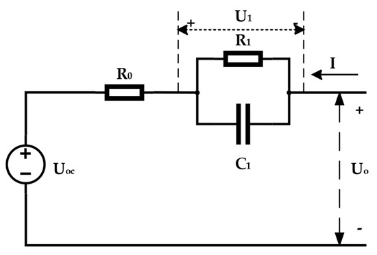
Figure 1.
Equivalent circuit model of LIBs (Remark: If the order of ECM changes, the algorithm can be applied to different ECMs after changing Equations (1)–(7), which are the input−output equations of the system).
The mathematical expression of ECM is a continuous equation, but BMS is used to identify parameters through sampling data points one after another. Therefore, Equations (1) and (2) need to be discretized into the form of difference equations.
Equation (2) is transformed into an expression in the frequency domain by Laplace variation.
Discrete Equations (3) and (4) are obtained. The derivation of omitted formula can be found in Ref. [28].
where T is denoted as sampling time, and a1, a2, and a3 can be written as
According to the description of the system equation in the FFRLS algorithm, the system output is defined as yk. The system input is defined as φk, and the parameter vector is defined as θk. The system equations can be obtained by rectification.
The FFRLS algorithm identification result θk contains parameters Uoc, a1, a2, and a3. However, the estimation of SOC actually requires parameters R0, R1, and C1. Accordingly, by inverting the result of Equation (5), Equation (7) can be obtained.
Additionally, the specific recursive process of FFRLS is expressed as Equation (8).
where K is the Kalman gain, P is the covariance matrix, and λ is the forgetting factor, which determines the sensitivity of discrimination result to system input.
2.2. Parameter Identification Based on VFFRLS
The LIBs of EVs usually work in complicated environments. When LIBs are current changing rapidly, the FFRLS algorithm with a fixed forgetting factor lacks sufficient accuracy [31,32,33]. If the forgetting factor λk can update in real time, the algorithm should be able to enhance accuracy and robustness.
This paper proposes a VFFRLS algorithm, which differs from FFRLS in forgetting factor λk. Forgetting factors in VFFRLS can be changed with the update of the innovation sequence. Therefore, the weights of new data can be adjusted in time to improve the accuracy of VFFRLS. In order to avoid a sudden increase in prediction error, VFFRLS sets a minimum forgetting factor and adds a data window m for the innovation sequence. Since the innovation sequence of FFRLS is limited, a sensitivity factor α is set to ensure the innovation sequence value is reasonable. The sensitivity of VFFRLS to innovation sequence shows a positive association with the sensitivity factor. Compared with FFRLS, the innovation of VFFRLS is shown in Equation (9). The overall flow of VFFRLS is shown in Algorithm 1.
| Algorithm 1. VFFRLS algorithm. |
|
3. SOC Estimation Based on ATEKF
Due to cost and other reasons, the accuracy of sensors in EVs is lower than that in laboratories. This leads to the measured voltage and current having a certain deviation from the real value in practical applications [34,35]. In the EKF algorithm, the measurement noise is used to reflect sensor error and interference noise, and the process noise to reflect the uncertainty of the prediction model. These uncertainties of noise greatly affect the accuracy of SOC estimation using EKF. These noises are difficult to quantify and variable in practical applications, so an adaptive correction mechanism has been proposed [36,37,38,39]. Based on existing research, this paper proposes an ATEKF algorithm, which can achieve adaptive correction of process noise, measurement noise, and covariance matrix. Therefore, it can improve the accuracy and robustness of SOC estimation.
For providing the state–space model of LIB, the model equation after discretization can be written as Equation (10).
where wk is the system process noise, vk is the measurement noise, f(·) is the state transfer function, and h(·) is the measurement function.
The state–space equation of the system can be obtained by Equations (1) and (2).
where , , , , .
Additionally, the detailed steps of EKF are as follows:
Step 1.
Initialize measurement noise R, process noise Q, covariance matrix P, and data window m1;
Step 2.
Using Equations (11) and (12), calculate the a priori state valueat k moment;
Step 3.
Calculate Kalman gainKk, error of prediction ek, and a priori state error covariance matrix;
Step 4.
Calculate a posteriori state value, and a posteriori state error covariance Pk;
where I is the unit matrix with the appropriate dimension.
Step 5.
Make k = k + 1 and return to Step 2; continue.
In order to enhance the accuracy of SOC estimation, AEKF adds the step of adaptively changing the process noise and measurement noise. However, it is worth noting that if data window m1 is not properly set, the AEKF algorithm will not converge.
By adding the following three equations between Step 4 and Step 5 of EKF, AEKF can be implemented.
where Hk represents innovation sequence; Pk and Qk represent measurement noise and process noise at k moment, respectively.
In the ATEKF algorithm, the innovation sequence is the basis of updating measurement noise, process noise, and covariance matrix. There is a reasonable relationship between innovation sequence and covariance matrix because the covariance matrix reflects the accuracy of estimation. Therefore, it is reasonable to correct the covariance matrix by innovation sequence [40].
The actual error can be defined as , and its calculation equation is written as Equation (21).
when , it means the accuracy of state estimation is high, and covariance matrix has to be reduced; when , it means that state estimation accuracy is inadequate, and covariance matrix should be increased. Nonetheless, in order to avoid divergence of estimated quantities, covariance matrix is kept constant.
Hence, we can decide whether to correct covariance matrix by comparing and Hk. The detailed calibration principle and correction factor are defined using Equation (22), where Tr(·) represents the function of solving matrix trace.
After adding the correction factor, Equation (13) can be rewritten as Equation (23)
From this deduction, the steps of ATEKF can be shown in Algorithm 2. The overall process of estimating SOC based on ATEKF is shown in Figure 2.
| Algorithm 2. ATEKF algorithm. |
|
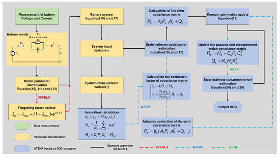
Figure 2.
Overall process of SOC estimation based on ATEKF.
4. Experimental Data
In this paper, the validation data were collected from a public dataset, which is measured by the University of Maryland [41]. Their experimental platform consists of test samples, a constant temperature chamber, an Arbin BT2000 battery test system, and a computer with Arbin software that collects voltage, current, charge, and discharge capacity data. The test sample was an 18,650 LiNiMnCoO2/Graphite battery, with a normal operating voltage of 3.6 V, nominal capacity of 2 Ah, maximum voltage and cut-off voltage of 4.2 V and 2.5 V, a maximum current of 22 A, and temperature ranging from 0 °C to 50 °C.
In this paper, we utilized five types of experiments included in the dataset. Among them, the incremental OCV test was used to establish the OCV–SOC function relationship. Additionally, the other four types were Federal Urban Driving Schedule (FUDS), Dynamic Stress Test (DST), Beijing Dynamic Stress Test (BJDST), and US06 Highway Driving Schedule. All experiments were conducted at 25 °C, with a sampling time of one second; their current data are shown in Figure 3. The OCV–SOC function relationship is defined as a polynomial in this paper, and the established parameters based on incremental OCV test data are shown in Table 1 [23].
where S represents the value of SOC.
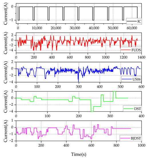
Figure 3.
Current data of battery experiments.

Table 1.
OCV–SOC fitting function parameters.
The single test times for DST, FUDS, BJDST, and US06 were only 360 s, 1372 s, 600 s, and 916 s. It is clear that the test would not have drained the battery if it ran only a single time. In order to collect enough data, the dynamic test in the dataset was run in cycles until the battery was depleted. There was a rest period of about 1 s between each cycle. The detailed definitions of these four dynamic tests can be found in the US Advanced Battery Consortium (USABC) manual and Environmental Protection Agency (EPA) manual.
5. Experimental Results
5.1. Verification of VFFRLS Performance
To demonstrate the performance of VFFRLS, DST and BJDST data were used to identify the ECM parameters. Additionally, the prediction error was compared with FFRLS. Figure 4 displays the variation of ECM parameters with SOC during the identification process. Figure 4a–d show the change in SOC, internal resistance R0, polarization resistor R1, and polarization capacitor C1, respectively. As shown in Figure 4b–d, some flickers exist with the main trend of the parameters. These fluctuations usually occur at the moment of rapid discharge and charge of DST conditions. The R1 and C1 reflect the internal polarization degree of the battery. When a battery is rapidly charged and discharged, its internal polarization degree varies widely, which leads to these flickers. Figure 5 shows the experimental situation of DST working conditions at 25 °C. The actual voltage, prediction voltage of FFRLS, and VFFRLS are shown in Figure 5a; in Figure 5b, the relative error of VFFRLS and FFRLS are compared. It can be seen that the error is mainly concentrated at the beginning and end of time, while the relative error of VFFRLS at the beginning is obviously smaller than FFRLS. Throughout the DST experiment, the average absolute error (MAE) of FFRLS is 0.045%, and the MAE of VFFRLS is 0.016%. Figure 5c shows the change in forgetting factor λ of VFFRLS during the DST experiment. It can be observed that the forgetting factor fluctuates more sharply at the beginning and end of the experiment, which is exactly in line with the design idea.
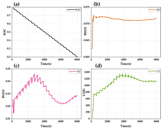
Figure 4.
Changes in parameters and SOC: (a) the change in SOC; (b) the change in internal resistance R0; (c) the change in polarization R1; (d) the change in polarization capacitor C1.
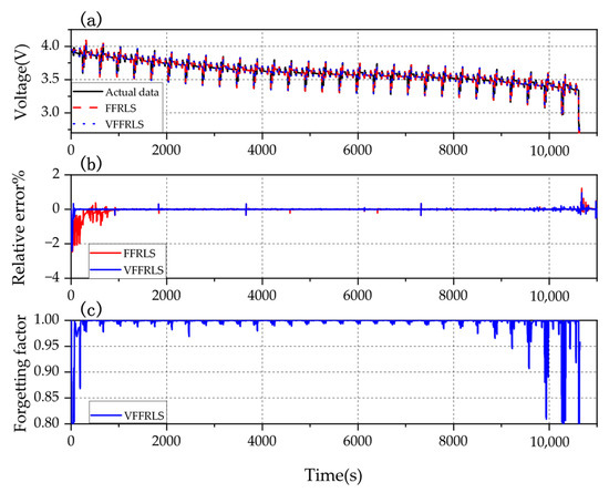
Figure 5.
DST under 25 °C: (a) actual voltage, predictive voltage of FFRLS, and VFFRLS; (b) relative error of VFFRLS and FFRLS; (c) forgetting factor λ of VFFRLS.
Figure 6 shows the experimental situation of the BJDST condition at 25 °C. The figure is approximately the same as Figure 5, and only Figure 6b is analyzed here. At the beginning of BJDST, the relative error of VFFRLS is still significantly smaller than FFRLS. The MAE of FFRLS is 0.05%, and the MAE of VFFRLS is 0.018% during the whole experiment. It is worth mentioning that forgetting factor λ set by FFRLS is 0.985, data window m1 set by VFFRLS is 10, sensitivity factor α set by VFFRLS is 20,000, and minimum forgetting factor λmin set by VFFRLS is 0.8.
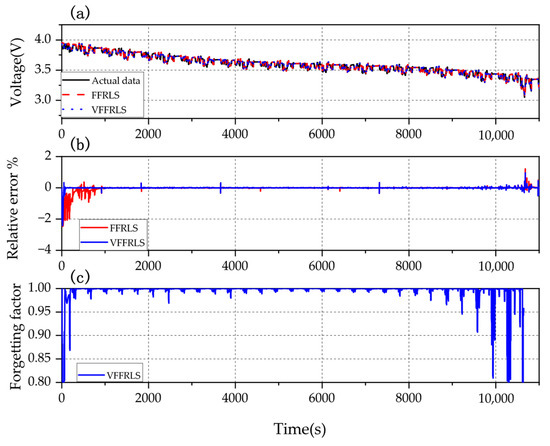
Figure 6.
BJDST under 25 °C: (a) actual voltage, predictive voltage of FFRLS and VFFRLS; (b) relative error of VFFRLS and FFRLS; (c) forgetting factor λ of VFFRLS.
5.2. Verification of ATEKF Performance
5.2.1. Accuracy of ATEKF
To reveal the accuracy of ATEKF, we compared the results of EKF and AEKF for four experiments. Figure 7 demonstrates the experimental result of DST at 25 °C. Figure 7a compares actual SOC and the prediction of EKF, AEKF, and ATEKF. The local magnification shows that the prediction of ATEKF is closest to the actual SOC. Figure 7b compares the prediction error of EKF, AEKF, and ATEKF, and the MAE values of them are 0.99%, 0.76%, and 0.47%, respectively. It can be observed that the prediction error of ATEKF stabilizes in a small range after a short time. However, the prediction error of EKF and AEKF have larger fluctuations. Figure 8, Figure 9 and Figure 10 are approximately the same as Figure 7 and simply show the prediction error of the three algorithms. Figure 8 shows the experimental result of FUDS at 25 °C. The MAE values of EKF, AEKF, and ATEKF are 1.09%, 0.75%, and 0.15%. Figure 9 displays the experimental result of BJDST at 25 °C. The MAE values of EKF, AEKF, and ATEKF are 0.78%, 0.76%, and 0.07%. Figure 10 exhibits the experimental result of US06 at 25 °C. The MAE values of EKF, AEKF, and ATEKF are 0.65%, 0.60%, and 0.32%.
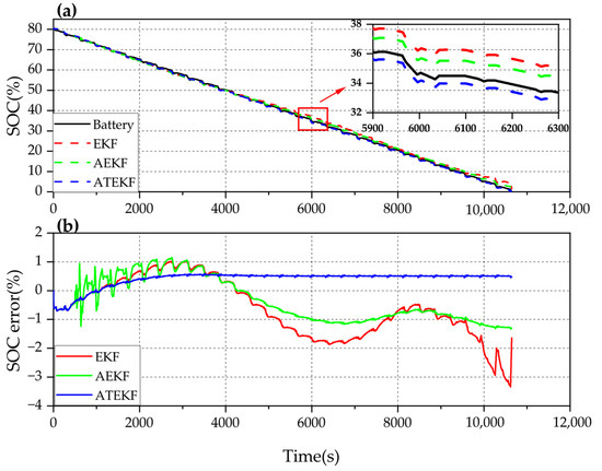
Figure 7.
DST under 25 °C: (a) actual SOC, prediction of EKF, AEKF, and ATEKF; (b) SOC error comparison of EKF, AEKF, and ATEKF.
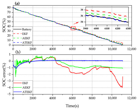
Figure 8.
FUDS under 25 °C: (a) actual SOC, prediction of EKF, AEKF, and ATEKF; (b) SOC error comparison of EKF, AEKF, and ATEKF.
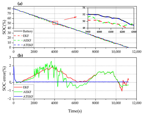
Figure 9.
BJDST under 25 °C: (a) actual SOC, prediction of EKF, AEKF, and ATEKF; (b) SOC error comparison of EKF, AEKF, and ATEKF.
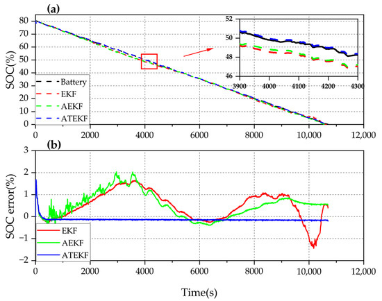
Figure 10.
US06 under 25 °C: (a) actual SOC, prediction of EKF, AEKF, and ATEKF; (b) SOC error comparison of EKF, AEKF, and ATEKF.
Combining these four figures and their MAEs, we can conclude that ATEKF outperforms the other two algorithms in SOC estimation. The data window m1 of VFFRLS is 1000 for the first two experiments and 100 for the last two experiments.
5.2.2. Robustness of ATEKF
In this paper, we compared the robustness of algorithms by adding voltage drift at different levels and setting different initialization of covariance matrices. Sensor errors are divided into two categories: drift and noise; however, the estimation error caused by noise can be reduced to zero in practical application. Therefore, we focused on the effect of voltage drift on SOC estimation, which is about 0.1%–1% [42,43,44]. Considering that the maximum voltage of an 18,650 battery is 4.2 V, voltage drift was taken from −40 mv to 40 mv. At the same time, considering that the state of health (SOH) of the battery impacts SOC, we compared the accuracy of EKF, AEKF, and ATEKF when SOH was from 70% to 90%.
Figure 11 shows the SOC estimation error of EKF, AEKF, and ATEKF for different degrees of voltage drift. Figure 11a shows the MAE data of SOC error in voltage drift intervals. It can be seen that ATEFK performs better than the other two algorithms in voltage drift conditions, and it is more obvious when drift voltage is large. By contrast, AEKF only outperforms EKF when drift voltage is positive, and the SOC estimation is not comparable to EKF when drift voltage is negative. Figure 11b–d show SOC estimation error for voltage drift of 20 mv, −5 mv, and 40 mv. In Figure 10b, the MAEs of EKF, AEKF, and ATEKF are 4.22%, 3.14%, and 2.07%, respectively. In Figure 11c, the MAEs of EKF, AEKF, and ATEKF are 0.72%, 0.42%, and 0.36%. In Figure 11d, the MAEs of EKF, AEKF, and ATEKF are 7.64%, 5.51%, and 4.12%.
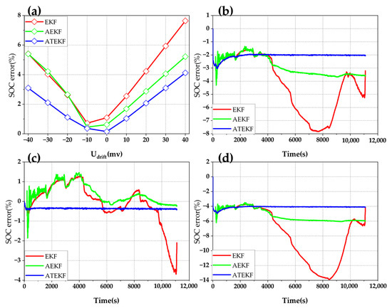
Figure 11.
SOC error of three algorithms with voltage drift: (a) MAEs of EKF, AEKF, and ATEKF with different voltage drifts; (b) SOC error comparison of EKF, AEKF, and ATEKF with 20 mv voltage drift; (c) SOC error comparison of EKF, AEKF, and ATEKF with −5 mv voltage drift; (d) SOC error comparison of EKF, AEKF, and ATEKF with 40 mv voltage drift.
The SOC estimation error of EKF, AEKF, and ATEKF for different measurement noises under FUDS conditions are shown in Figure 12. Figure 12a shows the MAE data of EKF, AEKF, and ATEKF under three measurement noises. It reveals that EKF is greatly influenced by measurement noise, whereas ATEKF is not sensitive to measurement noise. At the same time, ATEKF has higher accuracy, and AEKF is slightly inferior to EKF when . Figure 12b–d show SOC estimation error when , , and . In Figure 12b, the MAEs of EKF, AEKF, and ATEKF are 1.25%, 1.29%, and 0.17%. In Figure 12c, the MAEs of EKF, AEKF, and ATEKF are 0.57%, 0.51%, and 0.11%. In Figure 12d, the MAEs of EKF, AEKF, and ATEKF are 0.19%, 0.41%, and 0.14%.
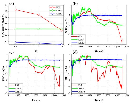
Figure 12.
SOC error of three algorithms under different measurement noises: (a) MAEs of EKF, AEKF, and ATEKF under different measurement noises; (b) SOC error comparison of EKF, AEKF, and ATEKF with ; (c) SOC error comparison of EKF, AEKF, and ATEKF with ; (d) SOC error comparison of EKF, AEKF, and ATEKF with .
Figure 13 shows the SOC error of EKF, AEKF, and ATEKF under different process noises. Figure 13a statistics the MAEs of EKF, AEKF, and ATEKF under different process noises. Among them, the performance of EKF is the most sensitive, and the accuracy of ATEKF is maintained to a wonderful degree regardless of the process noise. Figure 13b–d are SOC estimation errors when , , . In Figure 13b, the MAEs of EKF, AEKF, and ATEKF are 0.57%, 0.62%, and 0.11%. In Figure 13c, the MAEs of EKF, AEKF, and ATEKF are 1.09%, 0.62%, and 0.15%. In Figure 13d, the MAEs of EKF, AEKF, and ATEKF are 1.25%, 0.62%, and 0.17%.
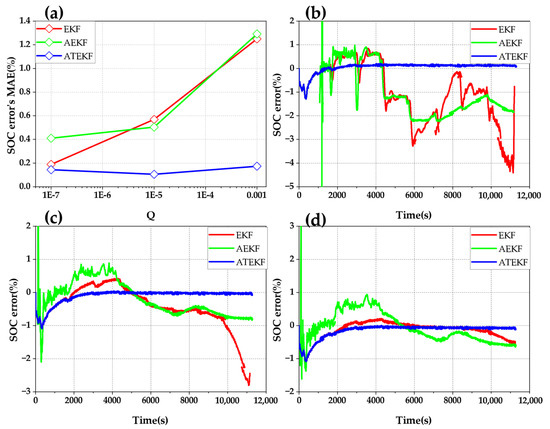
Figure 13.
SOC error of three algorithms under different process noises: (a) MAEs of EKF, AEKF, and ATEKF under different process noises; (b) SOC error comparison of EKF, AEKF, and ATEKF with ; (c) SOC error comparison of EKF, AEKF, and ATEKF with ; (d) SOC error comparison of EKF, AEKF, and ATEKF with .
Combining the three tests, we can observe that ATEKF can accurately estimate the LIB SOCs having voltage drift and covariance matrix uncertainty. Additionally, the accuracy of ATEKF is higher than EKF and AEKF in that case, which indicates that ATEKF has better robustness when having voltage drift and covariance matrix uncertainty.
Figure 14 displays the SOC error of EKF, AEKF, and ATEKF under different SOH. Figure 14a shows the MAE data of EKF, AEKF, and ATEKF with different SOH. The estimation error of EKF gradually increases with the decrease in SOH. However, the accuracy of AEKF and ATEKF are not as sensitive to SOH, since AEKF and ATEKF have adaptive correction mechanisms, which can update parameters by error. In SOH ranging from 90% to 70%, ATEKF has the best estimation results among the three algorithms. Figure 14b–d are SOC estimation errors when SOH values are 90%, 80%, and 70%. In Figure 14b, the MAEs of EKF, AEKF and ATEKF are 0.75%, 0.95% and 0.56%. In Figure 14c, the MAEs of EKF, AEKF and ATEKF are 0.94%, 1.02% and 0.68%. In Figure 14d, the MAEs of EKF, AEKF and ATEKF are 1.62%, 1.09% and 0.75%.
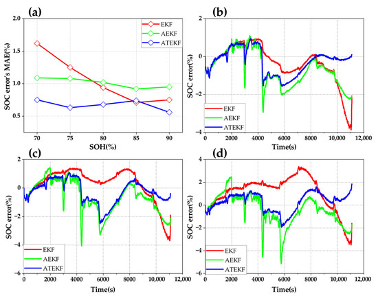
Figure 14.
SOC error of three algorithms under different SOH: (a) MAEs of EKF, AEKF, and ATEKF under different SOH; (b) SOC error comparison of EKF, AEKF, and ATEKF with SOH = 90%; (c) SOC error comparison of EKF, AEKF, and ATEKF with SOH = 80%; (d) SOC error comparison of EKF, AEKF, and ATEKF with SOH = 70%.
6. Conclusions
In order to solve some shortcomings of classical EKF in practical applications, we proposed two improvements in this paper. A VFFRLS algorithm was proposed to reduce the error of ECM, which can adaptively change the forgetting factor with the innovation sequence. Under BJDST conditions, the relative error of VFFRLS is 0.018%, and the relative of FFRLS is 0.05%. To improve the accuracy and robustness of SOC estimation, we proposed an ATEKF method. ATEKF can estimate the statistical properties of measurement noise and process noise by innovation sequence. Therefore, ATEKF has better accuracy and robustness than EKF and AEKF. Under FUDS conditions, the estimation error of EKF, AEKF, and ATEKF are 1.09%, 0.75%, and 0.15%. The estimation error of EKF, AEKF, and ATEKF are 7.64%, 5.51%, and 4.12% with 40 mv voltage drift.
In the future, the proposed method can be combined with other methods to solve problems in more practical situations. For example, a neural network can be trained to consider the effects of battery temperature and aging level. By combining this neural network with the proposed method, the accuracy of SOC estimation can be improved at different temperatures and aging levels.
Author Contributions
The study presented in this paper is a collaborative effort of the individual authors. K.G. and R.D. proposed the idea of the paper and wrote the original paper. D.M. and Y.M. designed proposed algorithms and accomplished the validation. Z.W. analyzed the data and supported the structure of the paper and revise the paper. All authors have read and agreed to the published version of the manuscript.
Funding
This research received no external funding.
Data Availability Statement
This study uses a publicly available dataset to validate the performance of the proposed algorithms. This lithium-ion battery dataset can be found here: https://web.calce.umd.edu/batteries/data.htm# (accessed on 28 December 2021).
Conflicts of Interest
The authors declare no conflict of interest.
References
- Liu, Y.; Liu, Y.; Chen, J. The impact of the Chinese automotive industry: Scenarios based on the national environmental goals. J. Clean. Prod. 2015, 96, 102–109. [Google Scholar] [CrossRef]
- Yong, J.Y.; Ramachandaramurthy, V.K.; Tan, K.M.; Mithulananthan, N. A review on the state-of-the-art technologies of electric vehicle, its impacts and prospects. Renew. Sustain. Energy Rev. 2015, 49, 365–385. [Google Scholar] [CrossRef]
- Hu, L.; Tian, Q.; Zou, C.; Huang, J.; Ye, Y.; Wu, X. A study on energy distribution strategy of electric vehicle hybrid energy storage system considering driving style based on real urban driving data. Renew. Sustain. Energy Rev. 2022, 162, 112416. [Google Scholar] [CrossRef]
- Iclodean, C.; Varga, B.; Burnete, N.; Cimerdean, D.; Jurchiş, B. Comparison of different battery types for electric vehicles. In IOP Conference Series: Materials Science and Engineering, Proceedings of the CAR2017 International Congress of Automotive and Transport Engineering-Mobility Engineering and Environment, Pitesti, Romania, 8–10 November 2017; IOP Publishing: Bristol, UK, 2017; Volume 252, p. 12058. [Google Scholar]
- Rawa, M.; Alghamdi, S.; Milyani, A.H.; Hariri, F.; Alghamdi, B.; Ajour, M.; Ćalasan, M.; Ali, Z.M.; Hasanien, H.M.; Popovic, B.; et al. Thermal model of supercapacitors operating in constant power applications: New mathematical expressions for precise calculation of temperature change. J. Energy Storage 2022, 49, 104121. [Google Scholar] [CrossRef]
- Ouyang, D.; Chen, M.; Liu, J.; Wei, R.; Weng, J.; Wang, J. Investigation of a commercial lithium-ion battery under overcharge/over-discharge failure conditions. RSC Adv. 2018, 8, 33414–33424. [Google Scholar] [CrossRef] [Green Version]
- Xiong, R.; Cao, J.; Yu, Q.; He, H.; Sun, F. Critical review on the battery state of charge estimation methods for electric vehicles. IEEE Access 2017, 6, 1832–1843. [Google Scholar] [CrossRef]
- Hannan, M.A.; Lipu, M.H.; Hussain, A.; Mohamed, A. A review of lithium-ion battery state of charge estimation and management system in electric vehicle applications: Challenges and recommendations. Renew. Sustain. Energy Rev. 2017, 78, 834–854. [Google Scholar] [CrossRef]
- Tang, X.; Wang, Y.; Chen, Z. A method for state-of-charge estimation of LiFePO4 batteries based on a dual-circuit state observer. J. Power Sources 2015, 296, 23–29. [Google Scholar] [CrossRef]
- Wei, M.; Ye, M.; Li, J.B.; Wang, Q.; Xu, X. State of charge estimation of lithium-ion batteries using LSTM and NARX neural networks. IEEE Access 2020, 8, 189236–189245. [Google Scholar] [CrossRef]
- Chandran, V.; Patil, C.K.; Karthick, A.; Ganeshaperumal, D.; Rahim, R.; Ghosh, A. State of charge estimation of lithium-ion battery for electric vehicles using machine learning algorithms. World Electr. Veh. J. 2021, 12, 38. [Google Scholar] [CrossRef]
- Tian, Y.; Lai, R.; Li, X.; Xiang, L.; Tian, J. A combined method for state-of-charge estimation for lithium-ion batteries using a long short-term memory network and an adaptive cubature Kalman filter. Appl. Energy 2020, 265, 114789. [Google Scholar] [CrossRef]
- Hu, L.; Ye, Y.; Bo, Y.; Huang, J.; Tian, Q.; Yi, X.; Li, Q. Performance evaluation strategy for battery pack of electric vehicles: Online estimation and offline evaluation. Energy Rep. 2022, 8, 774–784. [Google Scholar] [CrossRef]
- Beelen, H.; Bergveld, H.J.; Donkers, M.C.F. Joint estimation of battery parameters and state of charge using an extended Kalman filter: A single-parameter tuning approach. IEEE Trans. Control. Syst. Technol. 2020, 29, 1087–1101. [Google Scholar] [CrossRef]
- Hu, L.; Hu, X.; Che, Y.; Feng, F.; Lin, X.; Zhang, Z. Reliable state of charge estimation of battery packs using fuzzy adaptive federated filtering. Appl. Energy 2020, 262, 114569. [Google Scholar] [CrossRef]
- Xia, B.; Lao, Z.; Zhang, R.; Tian, Y.; Chen, G.; Sun, Z.; Wang, W.; Sun, W.; Lai, Y.; Wang, M.; et al. Online parameter identification and state of charge estimation of lithium-ion batteries based on forgetting factor recursive least squares and nonlinear Kalman filter. Energies 2017, 11, 3. [Google Scholar] [CrossRef] [Green Version]
- Yang, G.; Li, J.; Fu, Z.; Guo, L. Adaptive state of charge estimation of Lithium-ion battery based on battery capacity degradation model. Energy Procedia 2018, 152, 514–519. [Google Scholar] [CrossRef]
- Yang, S.; Zhou, S.; Hua, Y.; Zhou, X.; Liu, X.; Pan, Y.; Ling, H.; Wu, B. A parameter adaptive method for state of charge estimation of lithium-ion batteries with an improved extended Kalman filter. Sci. Rep. 2021, 11, 5805. [Google Scholar] [CrossRef]
- Zhu, Q.; Xu, M.; Liu, W.; Zheng, M. A state of charge estimation method for lithium-ion batteries based on fractional order adaptive extended kalman filter. Energy 2019, 187, 115880. [Google Scholar] [CrossRef]
- Li, Y.; Wang, C.; Gong, J. A combination Kalman filter approach for State of Charge estimation of lithium-ion battery considering model uncertainty. Energy 2016, 109, 933–946. [Google Scholar] [CrossRef]
- Yu, X.; Wei, J.; Dong, G.; Chen, Z.; Zhang, C. State-of-charge estimation approach of lithium-ion batteries using an improved extended Kalman filter. Energy Procedia 2019, 158, 5097–5102. [Google Scholar] [CrossRef]
- Lai, X.; Wang, S.; He, L.; Zhou, L.; Zheng, Y. A hybrid state-of-charge estimation method based on credible increment for electric vehicle applications with large sensor and model errors. J. Energy Storage 2020, 27, 101106. [Google Scholar] [CrossRef]
- Gandoman, F.H.; Ahmed, E.M.; Ali, Z.M.; Berecibar, M.; Zobaa, A.F.; Abdel Aleem, S.H. Reliability Evaluation of Lithium-Ion Batteries for E-Mobility Applications from Practical and Technical Perspectives: A Case Study. Sustainability 2021, 13, 11688. [Google Scholar] [CrossRef]
- Lai, X.; Zheng, Y.; Sun, T. A comparative study of different equivalent circuit models for estimating state-of-charge of lithium-ion batteries. Electrochim. Acta 2018, 259, 566–577. [Google Scholar] [CrossRef]
- Einhorn, M.; Conte, F.V.; Kral, C.; Fleig, J. Comparison, selection, and parameterization of electrical battery models for automotive applications. IEEE Trans. Power Electron. 2012, 28, 1429–1437. [Google Scholar] [CrossRef]
- Wang, Q.; Wang, J.; Zhao, P.; Kang, J.; Yan, F.; Du, C. Correlation between the model accuracy and model-based SOC estimation. Electrochim. Acta 2017, 228, 146–159. [Google Scholar] [CrossRef]
- Park, S.W.; Lee, H.; Won, Y.S. A novel aging parameter method for online estimation of Lithium-ion battery states of charge and health. J. Energy Storage 2022, 48, 103987. [Google Scholar] [CrossRef]
- Yan, L.; Peng, J.; Gao, D.; Wu, Y.; Liu, Y.; Li, H.; Liu, W.; Huang, Z. A hybrid method with cascaded structure for early-stage remaining useful life prediction of lithium-ion battery. Energy 2022, 243, 123038. [Google Scholar] [CrossRef]
- Du, R.; Hu, X.; Xie, S.; Hu, L.; Zhang, Z.; Lin, X. Battery aging-and temperature-aware predictive energy management for hybrid electric vehicles. J. Power Sources 2020, 473, 228568. [Google Scholar] [CrossRef]
- Wang, A.; Bian, H.; Wu, T. Research on SOC Estimation of Li Ion Battery Based on H∞-EKF Hybrid Filtering Algorithm. Master’s Thesis, Hubei University of Technology, Wuhan, China, 2021. [Google Scholar]
- Lao, Z.; Xia, B.; Wang, W.; Sun, W.; Lai, Y.; Wang, M. A novel method for lithium-ion battery online parameter identification based on variable forgetting factor recursive least squares. Energies 2018, 11, 1358. [Google Scholar] [CrossRef] [Green Version]
- Song, Q.; Mi, Y.; Lai, W. A novel variable forgetting factor recursive least square algorithm to improve the anti-interference ability of battery model parameters identification. IEEE Access 2019, 7, 61548–61557. [Google Scholar] [CrossRef]
- Sun, X.; Ji, J.; Ren, B.; Xie, C.; Yan, D. Adaptive forgetting factor recursive least square algorithm for online identification of equivalent circuit model parameters of a lithium-ion battery. Energies 2019, 12, 2242. [Google Scholar] [CrossRef] [Green Version]
- Lin, X. Theoretical analysis of battery SOC estimation errors under sensor bias and variance. IEEE Trans. Ind. Electron. 2018, 65, 7138–7148. [Google Scholar] [CrossRef]
- Xiong, R.; Yu, Q.; Shen, W.; Lin, C.; Sun, F. A sensor fault diagnosis method for a lithium-ion battery pack in electric vehicles. IEEE Trans. Power Electron. 2019, 34, 9709–9718. [Google Scholar] [CrossRef]
- Sepasi, S.; Ghorbani, R.; Liaw, B.Y. A novel on-board state-of-charge estimation method for aged Li-ion batteries based on model adaptive extended Kalman filter. J. Power Sources 2014, 245, 337–344. [Google Scholar] [CrossRef]
- Feng, L.; Ding, J.; Han, Y. Improved sliding mode based EKF for the SOC estimation of lithium-ion batteries. Ionics 2020, 26, 2875–2882. [Google Scholar] [CrossRef]
- Duan, J.; Wang, P.; Ma, W.; Qiu, X.; Tian, X.; Fang, S. State of Charge Estimation of Lithium Battery Based on Improved Correntropy Extended Kalman Filter. Energies 2020, 13, 4197. [Google Scholar] [CrossRef]
- Afshar, S.; Morris, K.; Khajepour, A. State-of-charge estimation using an EKF-based adaptive observer. IEEE Trans. Control. Syst. Technol. 2018, 27, 1907–1923. [Google Scholar] [CrossRef]
- Liu, M.; Cui, N.; Liu, S.; Wang, C.; Zhang, C.; Gong, S. Adaptive strong tracking unscented Kalman filter based SOC estimation for lithium-ion battery. In Proceedings of the 2017 Chinese Automation Congress (CAC), Jinan, China, 22–27 October 2017; pp. 1437–1441. [Google Scholar]
- Zheng, F.; Xing, Y.; Jiang, J.; Sun, B.; Kim, J.; Pecht, M. Influence of different open circuit voltage tests on state of charge online estimation for lithium-ion batteries. Appl. Energy 2016, 183, 513–525. [Google Scholar] [CrossRef]
- Liu, X.; Chen, Z.; Zhang, C.; Wu, J. A novel temperature-compensated model for power Li-ion batteries with dual-particle-filter state of charge estimation. Appl. Energy 2014, 123, 263–272. [Google Scholar] [CrossRef]
- Ouyang, M.; Gao, S.; Lu, L.; Feng, X.; Ren, D.; Li, J.; Zheng, Y.; Shen, P. Determination of the battery pack capacity considering the estimation error using a Capacity–Quantity diagram. Appl. Energy 2016, 177, 384–392. [Google Scholar] [CrossRef]
- Zheng, Y.; Ouyang, M.; Li, X.; Lu, L.; Li, J.; Zhou, L.; Zhang, Z. Recording frequency optimization for massive battery data storage in battery management systems. Appl. Energy 2016, 183, 380–389. [Google Scholar] [CrossRef]
Publisher’s Note: MDPI stays neutral with regard to jurisdictional claims in published maps and institutional affiliations. |
© 2022 by the authors. Licensee MDPI, Basel, Switzerland. This article is an open access article distributed under the terms and conditions of the Creative Commons Attribution (CC BY) license (https://creativecommons.org/licenses/by/4.0/).