1. Introduction
Hydroelectric power is a renewable energy source and a significant component of worldwide electricity production. Around 17% of the total consumed electricity is produced through hydraulic energy sources [
1,
2], and almost 65% of the total electricity produced in Latin America is generated by hydroelectric power plants (around 709 TWh/y) [
3,
4]. However, most of the total technical hydraulic potential (2859 TWh/y) of the region is not harnessed by its installed hydropower capacity. Several large-scale hydropower projects are being currently studied and developed in the Andean region in the hopes of increasing the installed capacity and harnessing a larger portion of the available hydraulic potential. One of the most crucial factors that needs to be taken into consideration during the development of the aforementioned projects is the fact that hard particles are present in almost all rivers of the Andean and Himalayan region, causing considerable the erosion, mechanical wear, and failure of turbine components [
3,
5].
Sediments flowing through the river deposit in the dam’s reservoir, reduce the reservoir’s capacity, and increase the erosion wear of critical turbine components, such as: the spiral casing, guide vanes, runner, and draft tube. This phenomenon reduces the lifespan of the turbine and decreases its efficiency, which increases the cost of maintenance over time, leading to economic losses [
6,
7]. Erosion wear depends on several factors, including particle concentration, velocity, composition, size, and shape. Other variables, namely turbine materials and operating conditions, also have an effect on the erosion rate. Therefore, erosion reduction strategies can only work effectively after in-depth analyses making a holistic assessment of all the variables involved [
8,
9].
Extensive research has been conducted on erosion in Francis turbines. In 2013, Singh and Banerjee performed an analysis on the erosion of the runner blades, guide vanes, and labyrinth seals of the Maneri Bhali Stage-II hydroelectric power plant in India. Data collection of sediments at relevant locations and measurements of turbine efficiency were performed during three years to determine the effect of silt erosion on the efficiency of turbines [
10]. In 2016, Koirala used a computational analysis coupled with field observations to determine the erosion patterns on the guide vanes of Kaligandaki hydroelectric power plant in Nepal and proposed erosion protection methods [
11]. A year later, Masoodi and Harmain presented a detailed comparison of two sediment-laden rivers and their effect on the runner blades of Himalayan hydroelectric power plants in India. A new erosion model was proposed in this study [
12]. Most recently, in 2020, Qian et al. executed a study on the erosion wear of the runner blades of a Francis turbine in Jhimruk Hydroelectric Center in Nepal using numerical simulations and comparing the results with the damage of the runners. He proposed changing the opening of the guide vanes to improve turbine efficiency and reduce the erosion rate [
13]. Moreover, Noon and Kim discussed and analyzed the latest experimental and numerical techniques to determine sediment and cavitation erosion on different turbine components using baseline data from the Tarbela Dam hydroelectric project in Pakistan [
14]. However, all the aforementioned studies were performed in Asia, and no research on the topic has been performed on South America, where similar erosion issues are found.
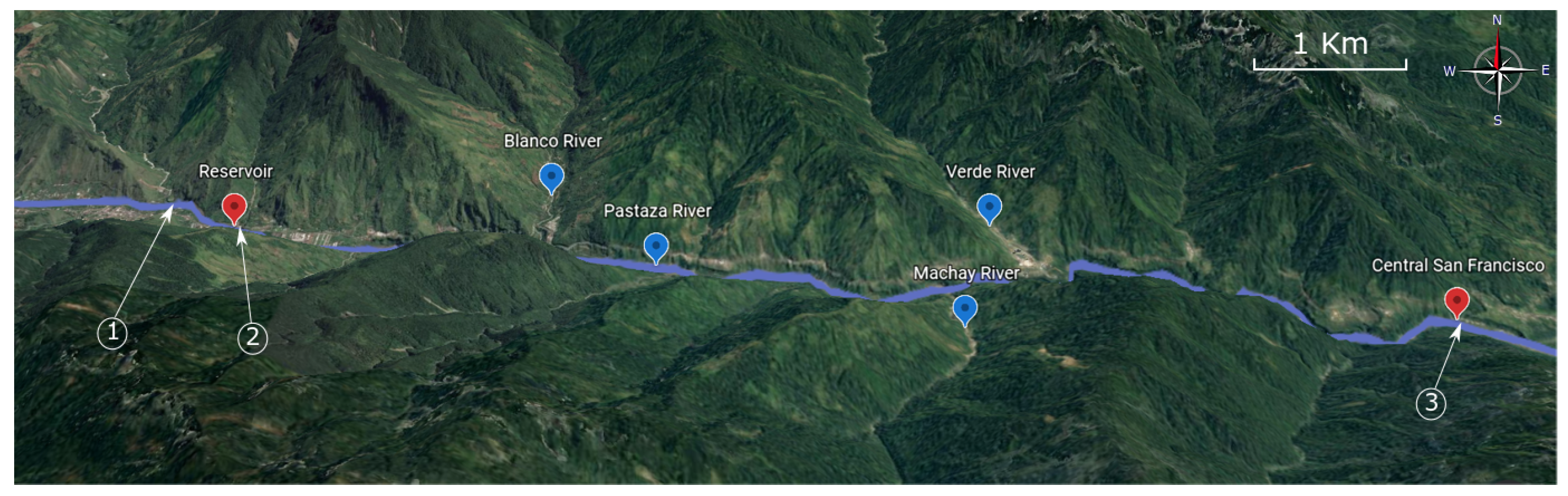
This study focuses on the analysis of sediment erosion in the Francis turbines of San Francisco hydroelectric power plant in Ecuador. The turbines of this power station suffer erosion wear damage, and to date, no effective strategies have been proposed to reduce the damage. A sediment characterization of the Pastaza River was conducted for this study in order to perform a numerical analysis of the turbines with sediment properties set as close as possible to the real conditions. Finally, a study on the erosion rate and pattern in different components of the turbine was carried out to better understand this phenomenon.
2. Case of Study: San Francisco Hydropower Plant
San Francisco hydro-power plant (SFH) is one of the largest energy generation centers in Ecuador, producing around 1140 GWh of electricity per annum, which represents 12% of the energy demand in the country. SFH is a 230 MW run-of-river hydropower plant located along Pastaza River, which consists of two vertical Francis turbines, each one running at 327.27 rpm under a net head of 213.4 m and a flow rate of 58 m
3/s. Since the plant began operations in 2007, it has suffered erosion problems, especially at the guide vanes and the outlet band of the runner.
Figure 1 presents a georeference of the plant.
2.1. Sediment Characterization at Pastaza River
The Pastaza River originates in the Andes mountains, where irregular geography and the presence of soft sediments due to high volcanic activity contribute to the high sediment content of South American rivers [
15]. These sediments pass through the turbines of hydraulic power plants, resulting in sediment erosion on exposed turbine components. To tackle the problems derived from erosion wear, an analysis of the particulate matter that flows through each power plant becomes necessary for a proper assessment of the erosion in a particular station. On this basis, the samples for the analysis were collected from the following zones of the hydropower plant:
The reservoir after the desilting chamber;
The outlet of the discharge gate;
The outlet of the draft tube.
2.1.1. Sediment Analysis
In order to characterize the particles of the Pastaza River at San Francisco hydropower plant, the collected sediment samples were analyzed at the Soil Mechanics and Materials Testing Laboratory, Escuela Politecnica Nacional, performing a sieve and composition analysis. The results of this analysis were considered during the study.
2.1.2. Particle Size and Distribution
A similar approach as the one followed by Koirala et al. [
11,
16] was used for this study. The sieve analysis was carried out under the ASTM D422-63 (2007) standard. Five sieve measurements of 4.75 mm, 2.00 mm, 0.85 mm, 0.425 mm, and 0.075 mm were used on five 120 g sediment samples.
Additionally, since particle roundness (R) and sphericity (S) affect most macroscale mechanical properties of the particle such as strength, compressibility, and shear wave velocity, it is necessary to estimate these parameters to increase the fidelity of the simulation [
17]. Roundness is described as the ratio between the average radius of curvature of the particle corners and the radius of the maximum inscribed circle, while sphericity is defined as the ratio of the particle width to particle length [
18]. The sphericity (spherical shape factor) and roundness of the particles were estimated using the Krumbein–Sloss chart [
19].
2.1.3. Mineral Composition Analysis
The mineral composition analysis for the study was performed through a particle count method using a D8 ADVANCE X-ray diffractometer and Diffrac plus software.
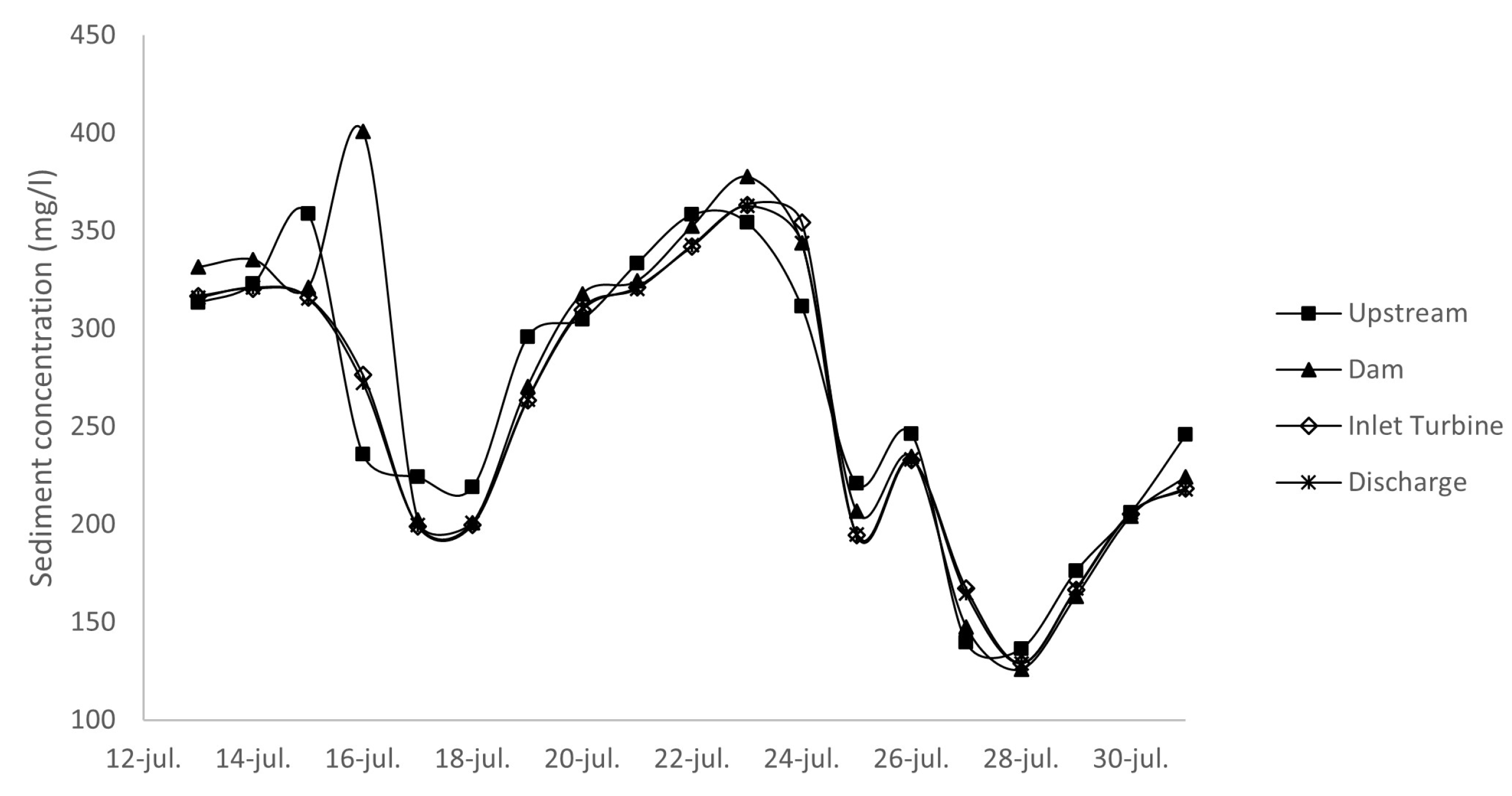
2.1.4. Sediment Concentration
Pastaza River is the third-largest river in Ecuador with an average annual flow 144.4 m
3/s and a precipitation of 3255 mm. Sediment concentration was determined based on data from San Francisco hydropower plant. The samples were collected daily 1 km upstream of the reservoir, in the reservoir itself, in the desilting chamber, and at the discharge during a month, as shown in
Figure 2. Since heavier particles tend to deposit on the reservoir bed and mostly only suspended particles are drawn by the intake, water samples were taken at a constant depth of about 2 m from the surface. The average concentration was estimated considering daily values from all sampling points throughout the sampling period.
3. Numerical Analysis of the Erosion in Francis Turbines
3.1. Governing Equations
3.1.1. Liquid Phase Mathematical Model
Fluids were calculated using a Eulerian approach. The general form of the equations involved in the calculations is presented. The mass continuity equation has the following form:
where:
The momentum conservation equation is shown in Equation (
2).
where:
pressure;
dynamic viscosity;
external forces.
3.1.2. Turbulence Model
A realizable k-
turbulence model was selected for its ability to correctly capture the turbulent nature of the flow in Francis turbines [
20,
21,
22]. This model was selected for its robustness and its improved boundary-layer-solving capacity under strong pressure gradients and flow separation compared to the standard k-
model [
23]. In addition, the k-
turbulence model has a low computational expense when compared to k-
SST. The transport equations for the realizable k-
take the following form:
where:
turbulent kinetic energy due to velocity gradients;
turbulent kinetic energy due to buoyancy;
contribution of compressible fluctuations to the dissipation rate;
constants;
Prandtl numbers;
Eddy dynamic viscosity;
user-defined terms.
The turbulence viscosity
is computed by:
Model variable
is defined by:
where
is the tensor for the mean rate of rotation in a reference frame rotating at an angular velocity
.
3.1.3. Solid Phase Mathematical Model
Solid particles were simulated using a Lagrangian approach and were treated as if their volume fraction were low compared to that of the continuous phase. Equation (
15) was derived from the force balance on the Lagrangian reference frame.
where:
The term
activates force terms in situations in which multiple reference frames are used and frame or mesh rotation is activated. The drag coefficient was estimated using the equations for the nonspherical drag law shown in Equation (
16).
where:
Particle dispersion caused by turbulent flows can be estimated using the stochastic tracking model [
24,
25]. This method, also known as the discrete random walk model, takes into account the effect of turbulent velocity fluctuations on the trajectories of particles. Instantaneous fluid velocity, as shown in Equation (
21), was used to integrate the particle trajectory equations along their path to predict the turbulent dispersion of particles. Random velocity fluctuations
were determined through Equation (
22), where
is a normally distributed random number. Particle diffusivity was estimated using Equation (
23), where the integral time scale as defined in Equation (
24) describes the time the particle remains in turbulent motion along a path
.
3.1.4. Erosion Model
The erosion model developed by Oka, Okamura, and Yoshida [
26,
27] was used to determine the erosion for the present case. This model is one of the most frequently used to determine the erosion in CFD analyses where solid particles suspended in a liquid medium are present [
28,
29,
30]. The equation developed by Oka is the following:
where:
erosion damage in ;
impact angle dependence of the normalized erosion;
erosion damage at a normal angle.
and:
where
Hv is the material Vickers hardness in GPa,
k is a velocity exponent,
k is a diameter exponent, and constants
n1 and
n2 are model exponents used to calculate the impact angle influence on the erosion rate.
D and
v are the reference diameter and velocity, respectively. The calibrated values of these parameters for the present case, in which sand particles and stainless steel were considered, are the ones presented in
Table 1.
3.2. Geometry and Conditions
Details of the general specifications of the turbine are presented in
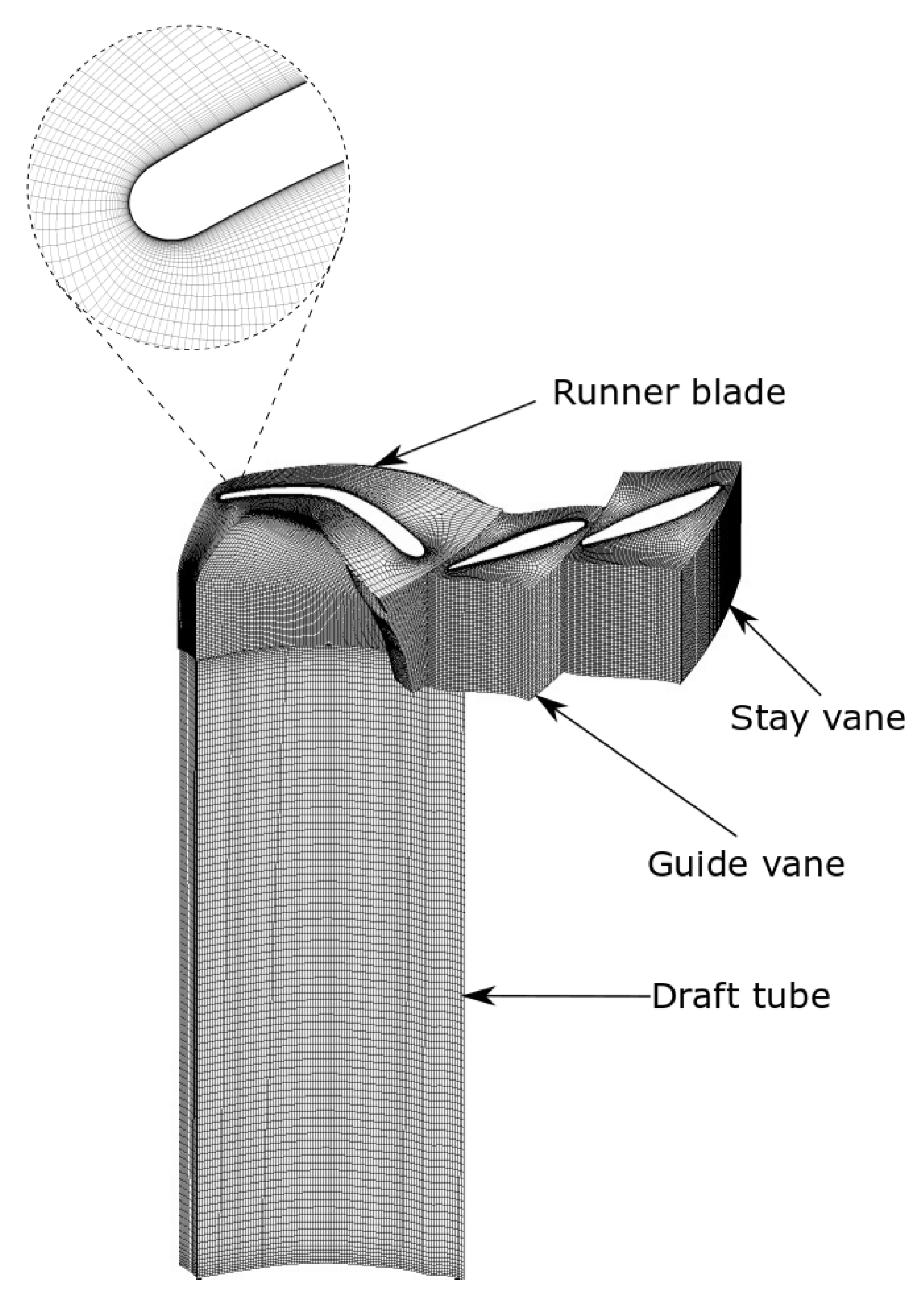
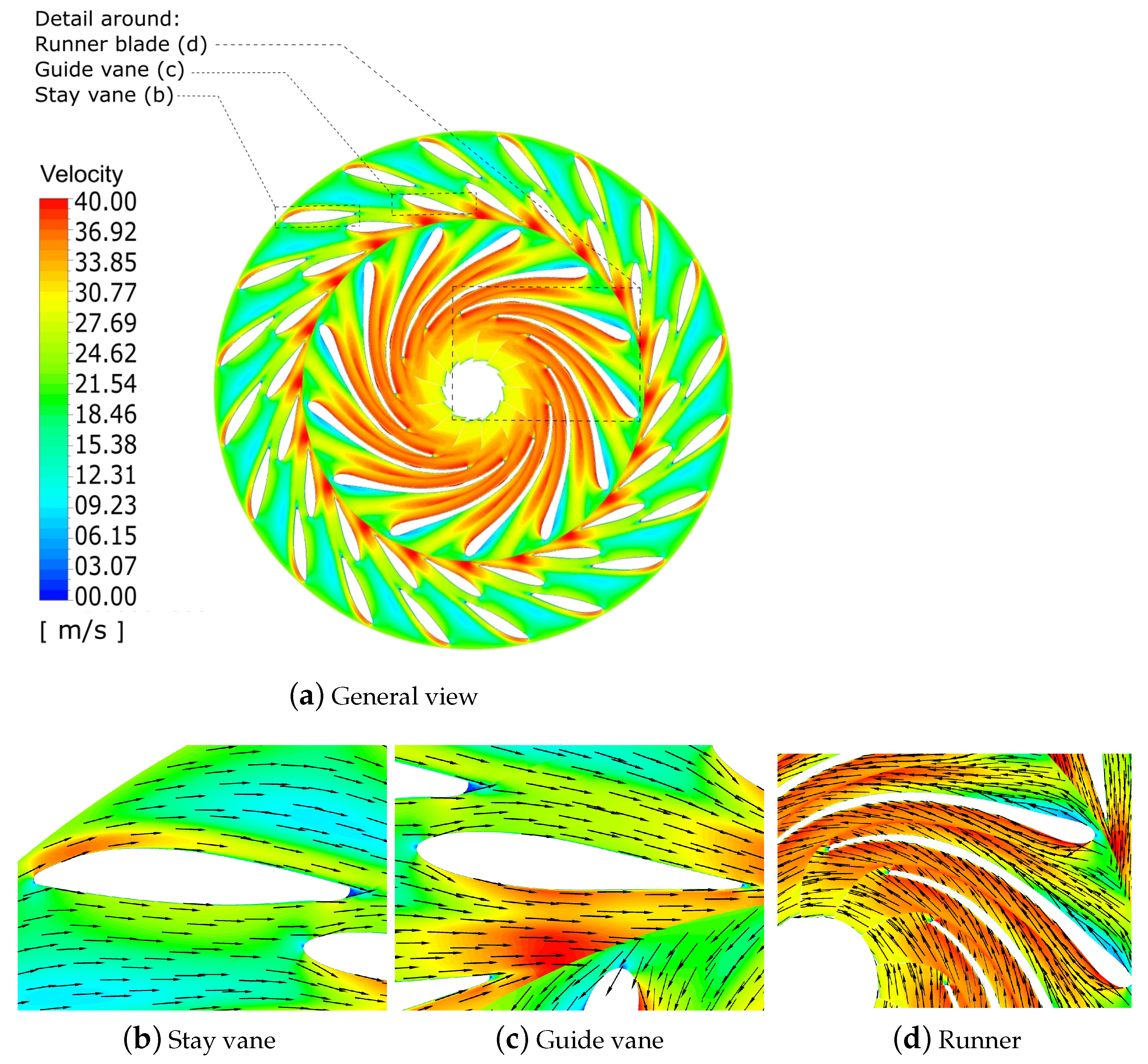
Table 2. In order to reduce the computational effort while using a more precise mesh for the numerical analysis, only one period of the turbine was simulated, which is comprises one stay vane, one guide vane, one runner blade, and an outlet domain representing the draft tube.
The computational domain is presented in
Figure 3. The geometry was obtained performing a 3D scanning of the turbine. The obtained profiles were reconstructed using ANSYS BladeGen to obtain a smoother geometry optimized for mesh construction using TurboGrid.
3.3. Operating Conditions
Table 3 shows the operating conditions that were used to perform the simulations. These conditions were translated to mass flow inlet and pressure outlet boundary conditions. The atmospheric pressure from the region was used to define the outlet pressure.
The characteristics of the sediments used for this study are shown in
Table 4. Particle mass flow rate was calculated as a function of the volumetric water flow rate of each case using the average particle concentration.
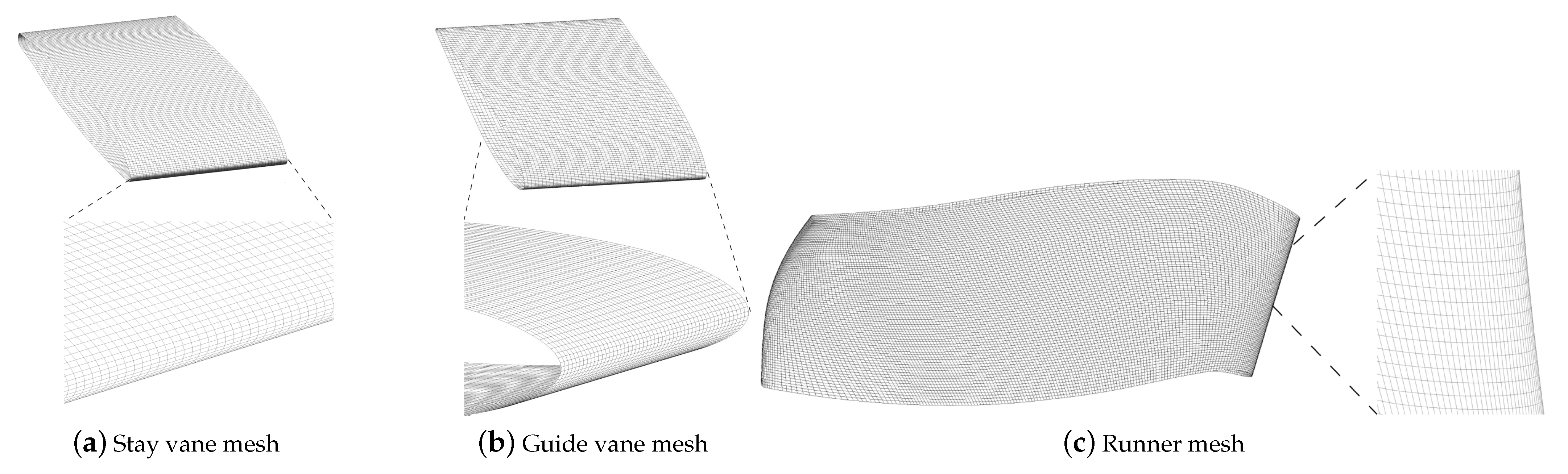
3.4. Mesh
The mesh was generated using the Turbogrid module, which employs a high-fidelity hexahedric structured mesh with a uniform distribution.
values were calculated for stay vanes, guide vanes, and runner blades through the following equation:
where
is the friction velocity,
y is the distance to the nearest wall, and
is the kinematic viscosity. The first cell height of each domain was calculated to correctly compute the boundary layer with the selected turbulence model, as shown in
Figure 3, by applying a locally refined region near the domain walls. The obtained
values ranged between 45 and 125, which are considered appropriate for the selected turbulence model [
31]. The quality of the mesh was also evaluated using the orthogonal quality model. The orthogonal quality of a cell was estimated as follows.
where:
face normal vector;
vector from the centroid of the cell to the centroid of the face;
vector from the centroid of the cell to the centroid of the adjacent cell.
A minimum orthogonal quality of 0.269 was obtained in 0.0000002% of mesh elements. The average orthogonal quality in all meshes was 0.93. The walls of the fully structured mesh are shown in
Figure 4Additionally, mesh independence studies were performed considering the pressure drop between the domain inlet and outlet. The structured mesh distribution was modified in all domain directions. Three different mesh resolutions were analyzed for each of the four individual operating conditions evaluated in the study. The results shown in
Figure 5 indicate that the difference between the calculations of the fine and medium mesh resolutions is negligible.
3.5. Solver
The numerical simulation was performed using the commercial software ANSYS Fluent. The present simulation used a RANS approach for the liquid phase through a realizable model. The dispersed phase was estimated using the discrete phase model in the commercial CFD software ANSYS Fluent. The numerical simulation was performed coupling all the subdomains with the following imposed boundary conditions:
The total mass flow inlet was designated at the inlet of the stay vane and the nonoverlapping interfaces of the runner;
A rotating frame was applied for the runner domain, and other regions were considered to be in a stationary frame;
Periodic repeats interfaces were created between the stay vane outlet and guide vane inlet and between the outlet of the runner and the inlet of the outlet domain;
A standard interface was created between the guide vane outlet and the inlet of the runner;
The total pressure was designated at the outlet of the runner;
Solid walls were set as nonslip boundary conditions.
A setup used previously in [
32] was used for the solid phase, where the injection was applied at the domain inlet and fully elastic collision was assumed at the walls. An analysis of the adequate number of particle injections was also carried out to generate a statistically meaningful sampling. One-hundred stochastic tracking tries were determined to be adequate to ensure that erosion on the walls of the turbine flow passage was independent of the number of injected particles.
The steady-state simulations were carried out using spatial derivatives discretized through a second-order upwind scheme. Full pressure–velocity coupling was enabled using the SIMPLE algorithm. Further, double precision was considered to improve the computational accuracy. A quantitative assessment of the discharge difference was made between the inlet and the outlet, which was lower than the order of .
The postprocessing phase was carried out in ANSYS CFD-Post, obtaining estimations of the erosion rate on the surfaces of the studied components. Additionally, the pressure and velocity of the flow were determined. Turbine efficiency was calculated based on these results.
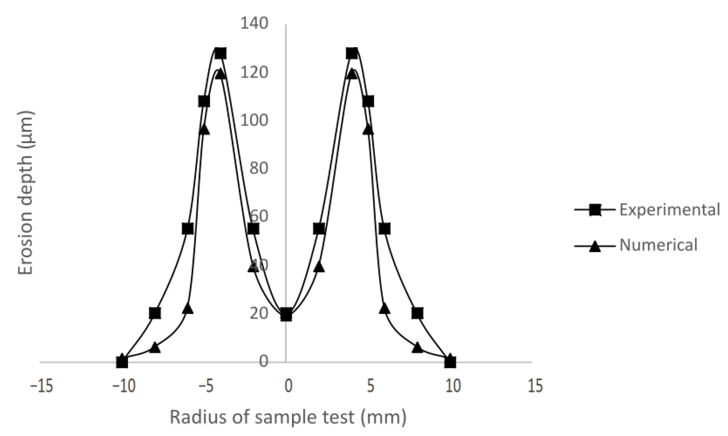
3.6. Validation
The study was validated by reproducing the numerical experiment of Nguyen [
28], where a wet erosion test rig was used to discharge and project sand particles. A stainless steel plate specimen with a 196 Vickers’ hardness was used for the experiment. The parameters of the experimental setup are shown in
Table 5.
The results shown in
Figure 6 were obtained from the numerical assessment. A satisfactory agreement between the erosion pattern and the results of the experimental and computational tests was observed.
The chart shows the material removal in the specimen caused by sediment erosion, where the center of the chart is aligned with the center of the nozzle. An inverted “W” shape was obtained for the erosion pattern caused by an expected stagnation point in the zone directly below the nozzle. The highest erosion rate was observed right outside this stagnation zone.
4. Results and Discussion
This section presents the results from the sediment analysis and the CFD analysis that were carried out to study the effect of sediment particles over the main components of SFH turbines when varying the guide vane opening. The simulation results were compared with actual site data.
4.1. Sediment Characterization
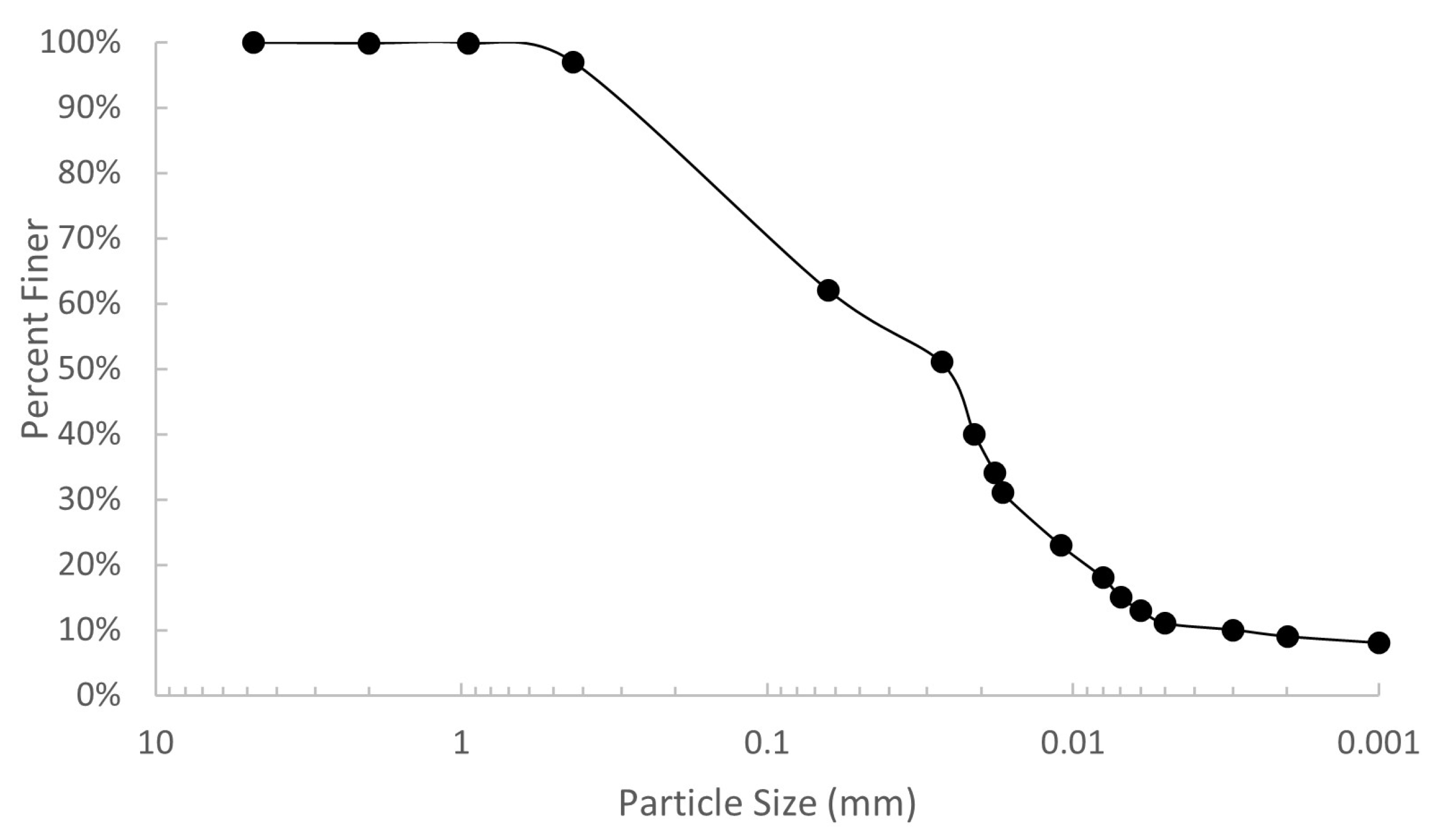
4.1.1. Particle Size
The analysis showed that 99.58% of the particles at the desilting basin were finer than 425 μm. In addition, the largest percentage (62.33%) of particles was finer than 75 μm.
Figure 7 shows the particle size distribution of the sediment samples. The median grain size was determined as 9.28 μm. Furthermore, the characterization of the particle density was performed, obtaining a value of 2650 kg/m
3.
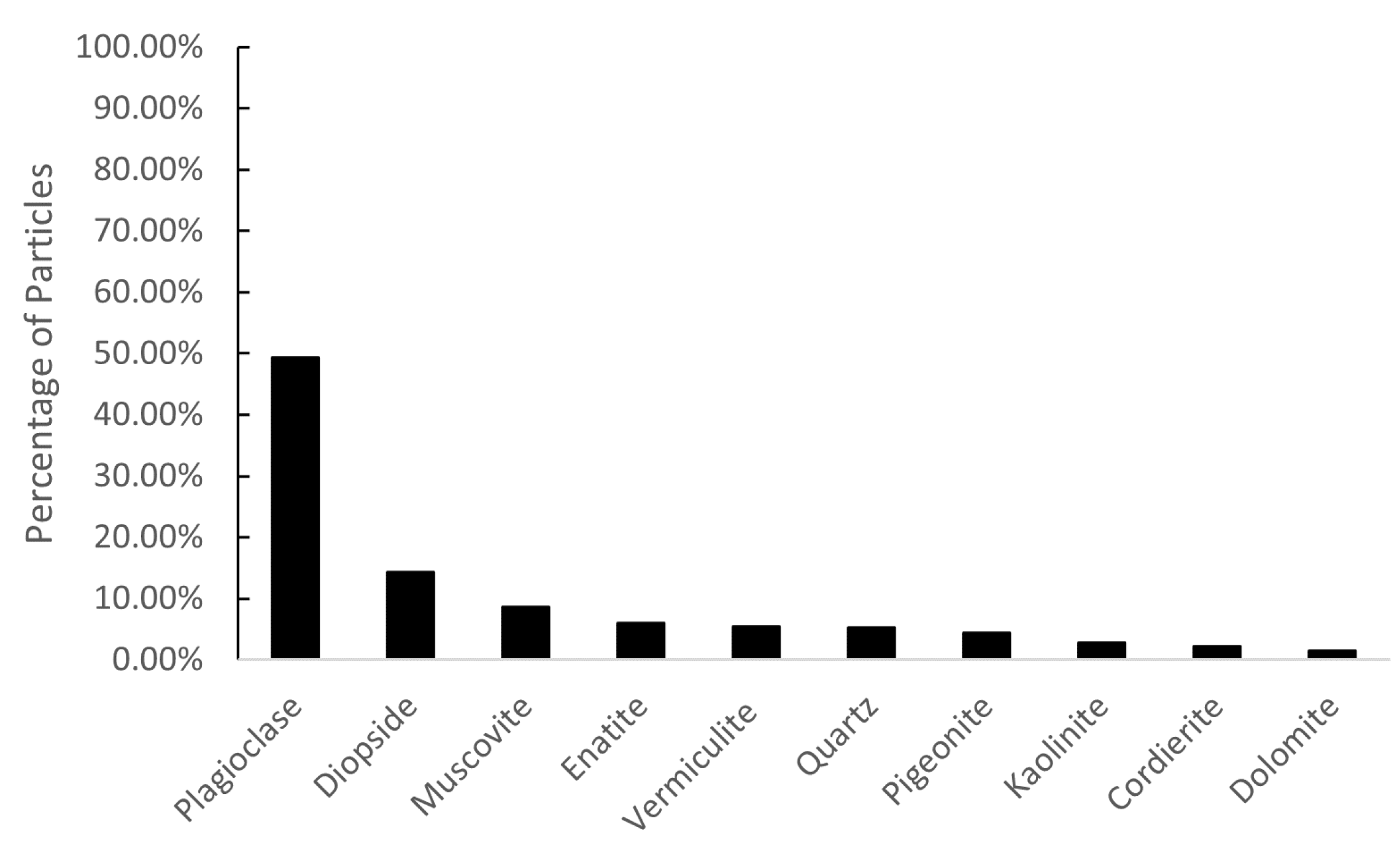
4.1.2. Mineral Composition
Figure 8 shows the proportion of the mineral content in sediment samples. The results showed that plagioclase minerals represented the highest proportion of sediments in the samples. The hardness values for this mineral group lies between 6.5 and 7.5 in the Mohs scale. When comparing this mineral composition to other reports, a difference in the proportion of quartz and plagioclase sediments was observed. Quartz is typically the predominant mineral found in most rivers, while in this study, plagioclase minerals composed the greatest part of the sediments found in Pastaza River. Nevertheless, the hardness values did not seem to differ significantly from other studies [
10,
11,
12,
14].
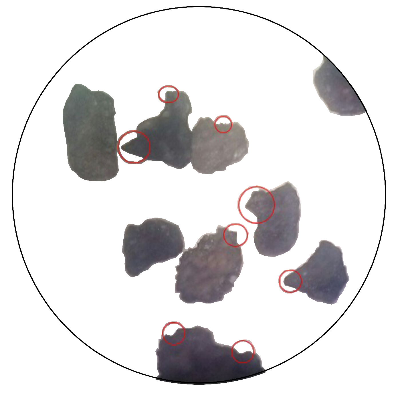
4.1.3. Particle Shape
Figure 9 presents the shape of the sediments found in the samples. The analysis exhibited the sharp and slightly rounded edges of the sample particles, which are equivalent to angular and subangular particles based on IEC 62364 standards [
33].
Comparing the shape of the sediments with the sample chart, the sphericity and roundness were found to be and , respectively.
4.1.4. Sediment Concentration
Table 6 shows particle concentration values in the river under normal conditions. The average concentration value was used to determine the particle mass flow rate.
4.2. Flow Field Prediction
Since erosion is governed by the velocity, incidence angle, and concentration of the solid particles at the time of collision, the erosion prediction depends on the solutions of these parameters.
Figure 10 presents the flow field in the turbine, where the main parameters that influence the sediment flow field are the inlet flow and the guide vane opening. In this context, the highest velocity of the flow was observed on the pressure side near the leading edge for the stay vanes. On the other hand, guide vanes and runner blades presented higher flow velocity on the suction side and trailing edge.
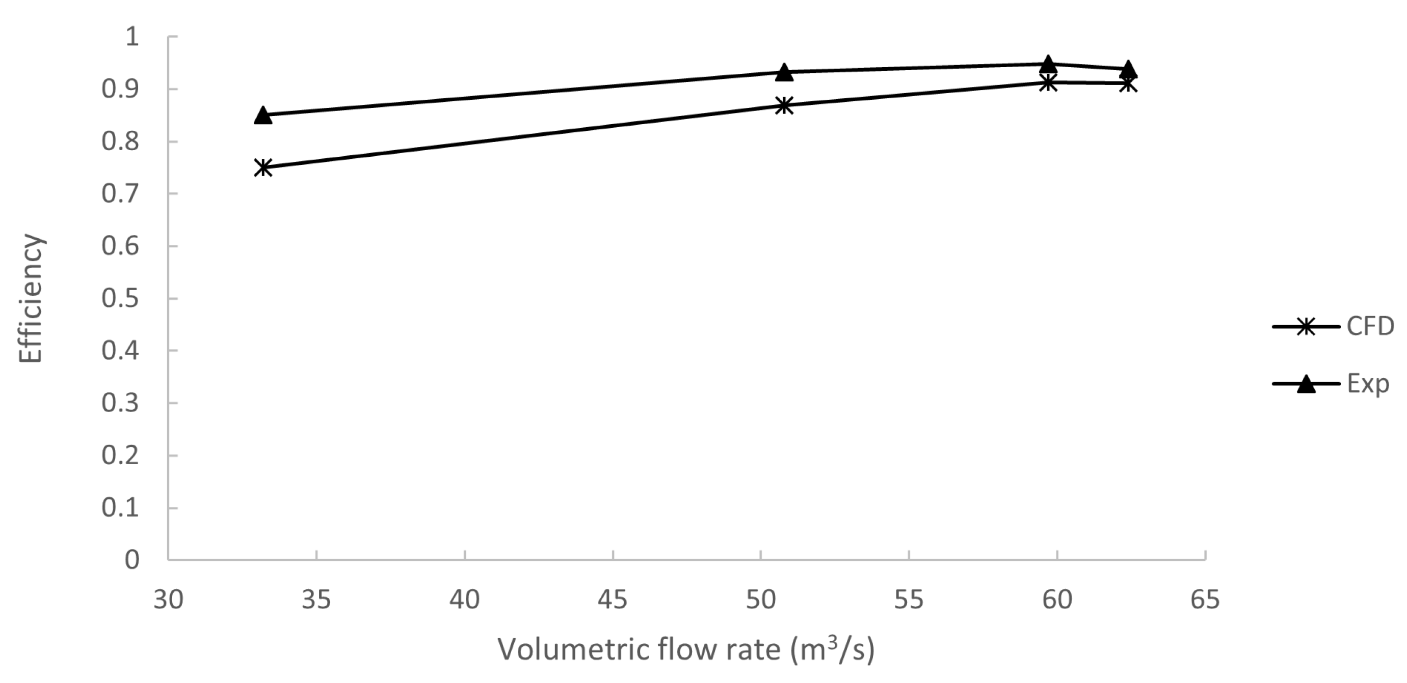
The efficiency of the turbine was calculated at four different operating points using the data from the flow numerical solution. These results were compared with the experimental data from SFH, as shown in
Figure 11.
Satisfactory agreement between results was obtained, though a better prediction of the efficiency was obtained for higher flow rates.
4.3. Sediment Erosion Prediction
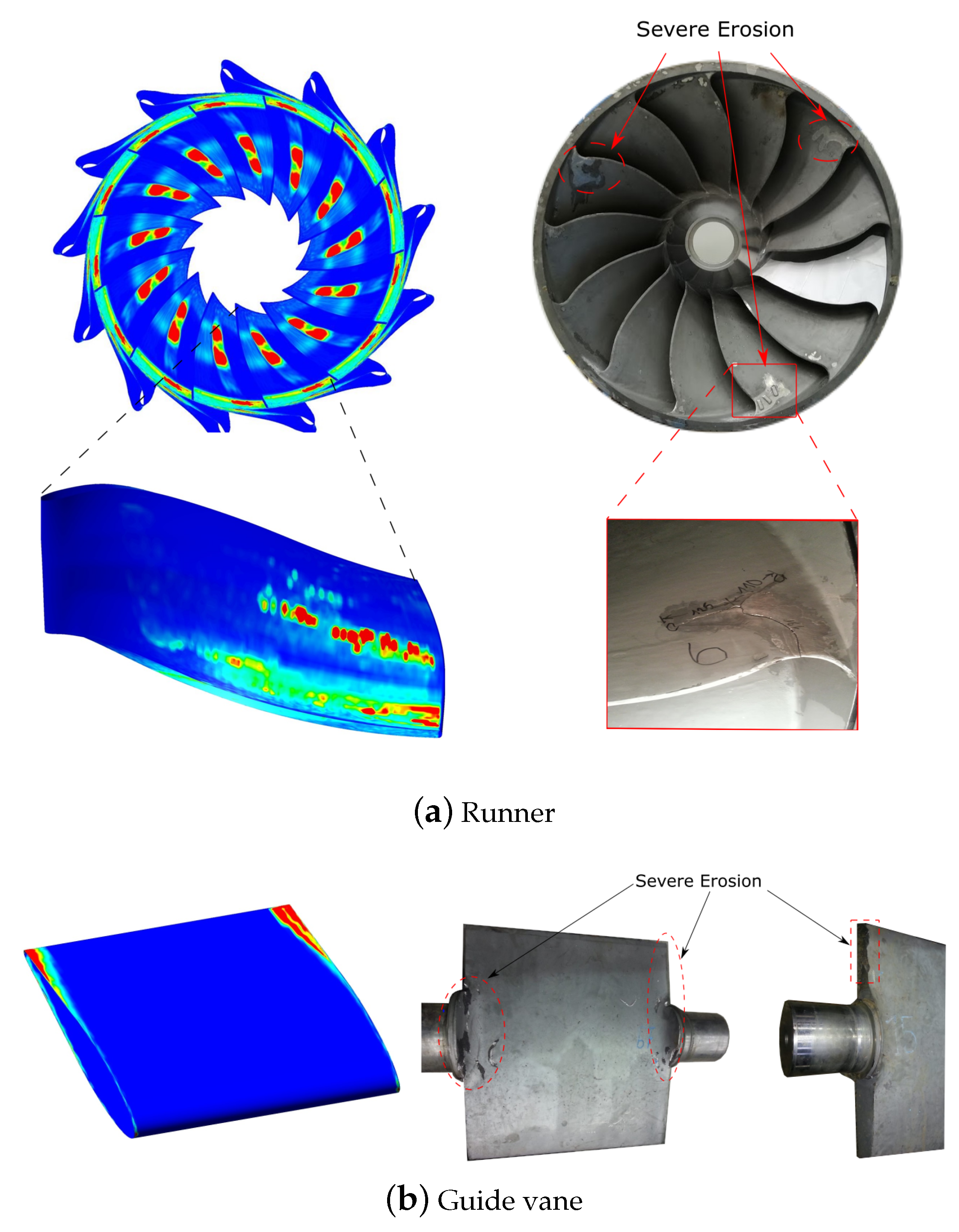
The sediment erosion patterns in critical turbine components are presented in
Figure 12. As seen in
Figure 12a, runner blades presented a higher erosion rate on the suction side near the trailing edge. In a similar manner, the guide vanes presented higher sediment erosion on the trailing edge of the suction side, as evidenced in
Figure 12b. Comparing the flow field from
Figure 10 with the eroded zones in
Figure 12, it is evident that zones with the highest relative flow velocity experienced higher erosion rates, as expected.
4.3.1. Erosion Description: San Francisco Francis Turbines
This section compares actual site erosion damage on the turbine with the results from the CFD analysis. The images on the right of
Figure 12 show the eroded components of a Francis turbine in SFH. Guide vanes presented a higher erosion rate near the clearance gap around the shaft and at both the leading and trailing edges of the vane since the inward flow accelerates near this region due to the decreasing net head pressure at the guide vane cascade. Regarding the runner, the most eroded areas were located at the leading edge and trailing edge of the blades due to the increase in particle velocity in these areas. Good agreement between numerical erosion results and site erosion was observed when comparing both components. The eroded areas of the runner blades coincided with the areas predicted by the numerical analysis. On the other hand, the eroded areas of the guide vanes did not match perfectly with the numerically predicted areas since the clearance gap near the hub and shroud that forces flow interaction with the shaft was not considered in this study.
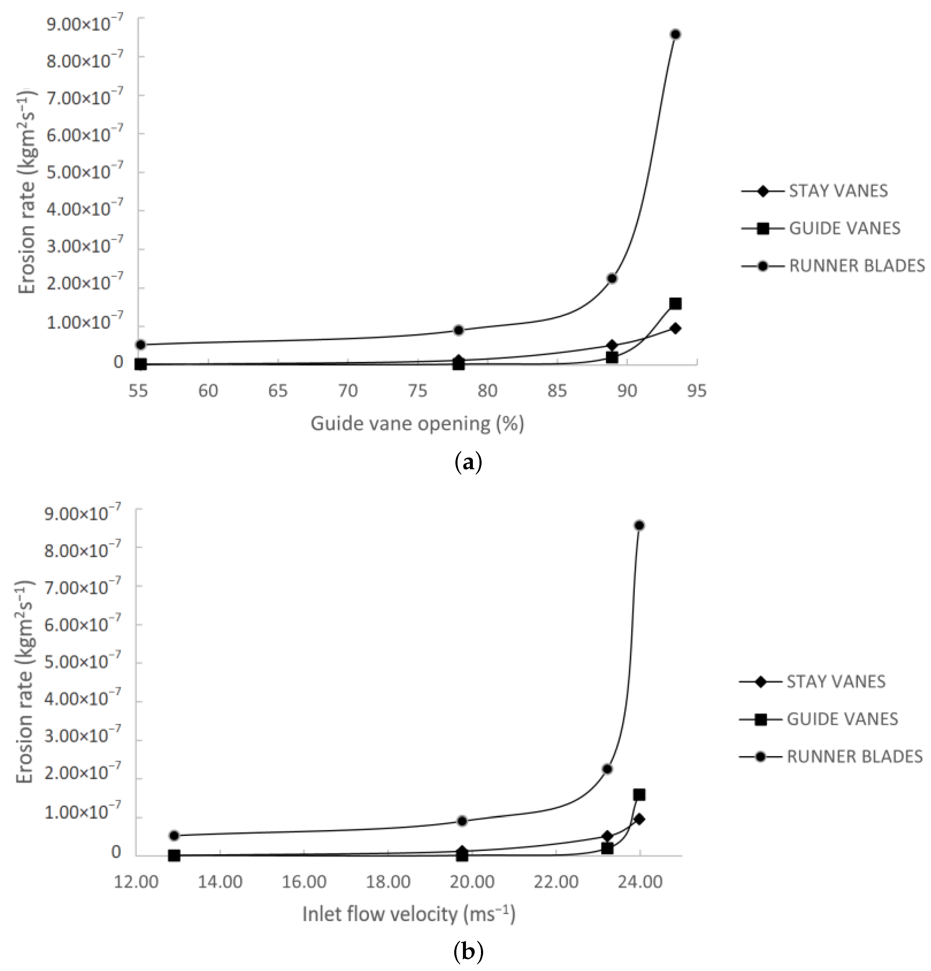
4.3.2. Effect of Operating Condition on the Erosion Rate
Figure 13 shows the influence of the guide vane opening and flow velocity on the erosion rate at the stay vanes, guide vanes, and runner. The erosion rate on the walls is calculated as:
where
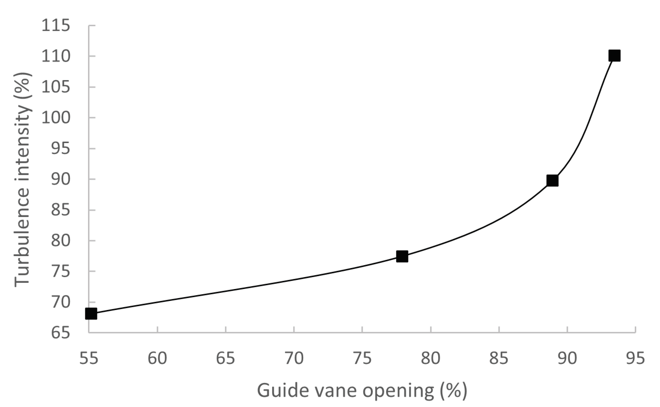
is the facet value of the erosion rate and A is the cell area. The erosion increases when increasing guide vane opening since the velocity and the amount of particles impacting the walls is multiplied due to the rise in water flow. A dramatic increase in the erosion rate was observed for operating conditions with guide vane openings over 90%. The sudden increase in erosion rate observed past a certain operating point may be related to the increase in the intensity of turbulent vortices near the outlet of the blade. Previous works [
34,
35] have found a direct relation among turbulent flow, vortex formation, and accelerated erosion. Vortices and recirculation accelerate particles in the flow and change the impingement angle to critical values.
Figure 14 shows the turbulence intensity of the flow surrounding the blade for the different operating conditions.
5. Conclusions
A CFD study replicating the operating conditions of the Francis turbines of San Francisco hydropower plant in Pastaza, Ecuador, was carried out. Flow conditions and erosion patterns were studied for different performance points, obtaining a detailed prediction of wear damage in different turbine components. From the results of the numerical analysis, the following can be concluded.
Erosion damage increases significantly for higher flow rates, when the opening of the guide vane exceeds an 85% aperture considering the closed position as a reference.
Operating the turbines at the previously mentioned conditions would result in unnecessary and accelerated erosion wear since the best performance point was obtained at a lower flow rate.
The operation of Francis turbines in sediment-laden rivers should be carried out with particular consideration of the effect that guide vane opening has on the formation of turbulent flow and vorticity. This situation can lead to accelerated erosion rates since vortices and recirculation can accelerate particles in the flow and change the impingement angle to critical values.
CFD is a powerful tool that can be used to prevent such occurrences and analyze the operating conditions in hydropower plants that best harness the available power without sacrificing mechanical integrity.
This study was conducted with the aim of contributing to the creation of a clear and cost-effective strategy to prevent and reduce erosion in existing hydropower plants and proposing an effective erosion-based operating procedure for Francis turbines in the Andean region.
Author Contributions
Conceptualization, E.C.; methodology, E.C. and E.V.; software, C.C.; validation, C.C.; formal analysis, C.C. and D.J.; investigation, C.C. and D.J.; resources, E.C., C.M. and E.V.; data curation, E.V.; writing—original draft preparation, C.C. and D.J.; writing—review and editing, C.C., E.C., E.V. and X.L.; visualization, C.C. and D.J.; supervision, E.C. and I.Z.; project administration, E.C. and I.Z.; funding acquisition, E.C. All authors have read and agreed to the published version of the manuscript.
Funding
This research was funded by Escuela Politécnica Nacional (PIS 19-06).
Institutional Review Board Statement
Not applicable.
Informed Consent Statement
Not applicable.
Acknowledgments
The authors gratefully acknowledge the financial support provided by Escuela Politécnica Nacional through the project PIS 19-06.
Conflicts of Interest
The authors declare no conflict of interest.
References
- Gernaat, D.E.; Bogaart, P.W.; van Vuuren, D.P.; Biemans, H.; Niessink, R. High-resolution assessment of global technical and economic hydropower potential. Nat. Energy 2017, 2, 821–828. [Google Scholar] [CrossRef]
- Sipahutar, R.; Bernas, S.M.; Imanuddin, M.S. Renewable energy and hydropower utilization tendency worldwide. Renew. Sustain. Energy Rev. 2013, 17, 213–215. [Google Scholar]
- Killingtveit, Å. 15-Hydroelectric Power. In Future Energy, 3rd ed.; Letcher, T.M., Ed.; Elsevier: Amsterdam, The Netherlands, 2020; pp. 315–330. [Google Scholar] [CrossRef]
- Hoes, O.A.; Meijer, L.J.; Van Der Ent, R.J.; Van De Giesen, N.C. Systematic high-resolution assessment of global hydropower potential. PLoS ONE 2017, 12, e0171844. [Google Scholar] [CrossRef]
- Koirala, R.; Zhu, B.; Neopane, H.P. Effect of guide vane clearance gap on Francis turbine performance. Energies 2016, 9, 275. [Google Scholar] [CrossRef]
- Noon, A.A.; Kim, M.H. Erosion wear on Francis turbine components due to sediment flow. Wear 2017, 378, 126–135. [Google Scholar] [CrossRef]
- Levy, A.V. The solid particle erosion behavior of steel as a function of microstructure. Wear 1981, 68, 269–287. [Google Scholar] [CrossRef]
- Thapa, B.S.; Thapa, B.; Dahlhaug, O.G. Empirical modelling of sediment erosion in Francis turbines. Energy 2012, 41, 386–391. [Google Scholar] [CrossRef]
- Thapa, B.S.; Gjosater, K.; Eltvik, M.; Dahlhaug, O.G.; Thapa, B. Effects of turbine design parameters on sediment erosion of Francis runner. In Proceedings of the 2nd International Conference on the Developments in Renewable Energy Technology (ICDRET 2012), Dhaka, Bangladesh, 5–7 January 2012; pp. 1–5. [Google Scholar]
- Singh, M.; Banerjee, J.; Patel, P.; Tiwari, H. Effect of silt erosion on Francis turbine: A case study of Maneri Bhali Stage-II, Uttarakhand, India. ISH J. Hydraul. Eng. 2013, 19, 1–10. [Google Scholar] [CrossRef]
- Koirala, R.; Thapa, B.; Neopane, H.P.; Zhu, B.; Chhetry, B. Sediment erosion in guide vanes of Francis turbine: A case study of Kaligandaki Hydropower Plant, Nepal. Wear 2016, 362, 53–60. [Google Scholar] [CrossRef]
- Masoodi, J.; Harmain, G. Sediment erosion of Francis turbine runners in the Himalayan region of India. Int. J. Hydropower Dams 2017, 24, 82–89. [Google Scholar]
- Qian, Z.; Zhao, Z.; Guo, Z.; Thapa, B.S.; Thapa, B. Erosion wear on runner of Francis turbine in Jhimruk Hydroelectric Center. J. Fluids Eng. 2020, 142, 094502. [Google Scholar] [CrossRef]
- Noon, A.A.; Kim, M.H. Sediment and Cavitation Erosion in Francis Turbines—Review of Latest Experimental and Numerical Techniques. Energies 2021, 14, 1516. [Google Scholar] [CrossRef]
- Laraque, A.; Bernal, C.; Bourrel, L.; Darrozes, J.; Christophoul, F.; Armijos, E.; Fraizy, P.; Pombosa, R.; Guyot, J.L. Sediment budget of the Napo river, Amazon basin, Ecuador and Peru. Hydrol. Process. Int. J. 2009, 23, 3509–3524. [Google Scholar] [CrossRef] [Green Version]
- Koirala, R.; Chitrakar, S.; Regmi, S.N.; Khadka, M.; Thapa, B.; Neopane, H.P. Analysis of sediment samples and erosion potential: A case study of Upper Tamakoshi Hydroelectric Project. Hydro Nepal 2015, 16, 28–31. [Google Scholar] [CrossRef]
- Cruz-Matías, I.; Ayala, D.; Hiller, D.; Gutsch, S.; Zacharias, M.; Estradé, S.; Peiró, F. Sphericity and roundness computation for particles using the extreme vertices model. J. Comput. Sci. 2019, 30, 28–40. [Google Scholar] [CrossRef]
- Hryciw, R.D.; Zheng, J.; Shetler, K. Particle roundness and sphericity from images of assemblies by chart estimates and computer methods. J. Geotech. Geoenviron. Eng. 2016, 142, 04016038. [Google Scholar] [CrossRef]
- Krumbein, W.C.; Sloss, L.L. Stratigraphy and Sedimentation; W.H. Freeman & Co.: San Francisco, CA, USA, 1951; pp. 114–128. [Google Scholar]
- Stoessel, L.; Nilsson, H. Steady and unsteady numerical simulations of the flow in the Tokke Francis turbine model, at three operating conditions. J. Phys. Conf. Ser. 2015, 579, 012011. [Google Scholar] [CrossRef] [Green Version]
- Iovănel, R.; Bucur, D.; Cervantes, M. Study on the Accuracy of RANS Modelling of the Turbulent Flow Developed in a Kaplan Turbine Operated at BEP. Part 1—Velocity Field. J. Appl. Fluid Mech. 2019, 12, 1449–1461. [Google Scholar] [CrossRef]
- Liu, H.L.; Liu, M.M.; Dong, L.; Ren, Y.; Du, H. Effects of computational grids and turbulence models on numerical simulation of centrifugal pump with CFD. IOP Conf. Ser. Earth Environ. Sci. 2012, 15, 062005. [Google Scholar] [CrossRef] [Green Version]
- ANSYS Inc. ANSYS Fluent User’s Guide, R2014, Section 4.4.3; ANSYS, Inc.: Canonsburg, PA, USA, 2014. [Google Scholar]
- ANSYS Inc. ANSYS Fluent User’s Guide, R2014, Section 15.2.2; ANSYS, Inc.: Canonsburg, PA, USA, 2014. [Google Scholar]
- Huilier, D.G.F. An Overview of the Lagrangian Dispersion Modeling of Heavy Particles in Homogeneous Isotropic Turbulence and Considerations on Related LES Simulations. Fluids 2021, 6, 145. [Google Scholar] [CrossRef]
- Oka, Y.; Yoshida, T.; Okamura, K. Practical estimation of erosion damage caused by solid particle impact, Part 1: Effects of impact parameters on a predictive equation. Wear 2005, 259, 95–101. [Google Scholar] [CrossRef]
- Oka, Y.; Yoshida, T. Practical estimation of erosion damage caused by solid particle impact Part 2: Mechanical properties of materials directly associated with erosion damage. Wear 2005, 259, 102–109. [Google Scholar] [CrossRef]
- Nguyen, V.; Nguyen, Q.; Liu, Z.; Wan, S.; Lim, C.; Zhang, Y. A combined numerical–experimental study on the effect of surface evolution on the water–sand multiphase flow characteristics and the material erosion behavior. Wear 2014, 319, 96–109. [Google Scholar] [CrossRef]
- Pereira, G.; de Souza, F.; de Moro Martins, D. Numerical prediction of the erosion due to particles in elbows. Powder Technol. 2014, 261, 105–117. [Google Scholar] [CrossRef]
- Messa, G.; Wang, Y. Importance of accounting for finite particle size in CFD-based erosion prediction. Powder Technol. 2014, 261, 105–117. [Google Scholar]
- Cando, E.; Yu, A.; Zhu, L.; Liu, J.; Lu, L.; Hidalgo, V.; Luo, X.W. Unsteady numerical analysis of the liquid–solid two-phase flow around a step using Eulerian-Lagrangian and the filter-based RANS method. J. Mech. Sci. Technol. 2017, 31, 2781–2790. [Google Scholar] [CrossRef]
- Cando, E.; Huan, R.F.; Valencia, E.; Luo, X.W. Sediment Erosion Prediction for a Francis Turbine Based on Liquid-Solid Flow Simulation Using Modified PANS. In Proceedings of the 4th World Congress on Mechanical, Chemical, and Material Engineering, Madrid, Spain, 16–18 August 2018. [Google Scholar]
- Hydraulic Machines-Guidelines for Dealing with Hydro-Abrasive Erosion in Kaplan, Francis, and Pelton Turbines, IEC 62634. 2019. Available online: https://webstore.iec.ch/preview/info_iec62364%7Bed2.0.RLV%7Den.pdf (accessed on 10 August 2021).
- Chen, Y.; Li, R.; Han, W.; Guo, T.; Su, M.; Wei, S. Sediment Erosion Characteristics and Mechanism on Guide Vane End-Clearance of Hydro Turbine. Appl. Sci. 2019, 9, 4137. [Google Scholar] [CrossRef] [Green Version]
- Neopane, H.P.; Dahlhaug, O.G.; Cervantes, M. The effect of sediment characteristics for predicting erosion on Francis turbines blades. Int. J. Hydropower Dams 2012, 19, 79–83. [Google Scholar]
Figure 1.
San Francisco hydroelectric power plant location.
Figure 1.
San Francisco hydroelectric power plant location.
Figure 2.
Sediment concentration in July 2010.
Figure 2.
Sediment concentration in July 2010.
Figure 3.
Computational domain of San Francisco’s Francis turbine.
Figure 3.
Computational domain of San Francisco’s Francis turbine.
Figure 4.
Mesh of the conceptual model.
Figure 4.
Mesh of the conceptual model.
Figure 5.
Mesh independence analysis.
Figure 5.
Mesh independence analysis.
Figure 6.
Numerical and experimental material removal in the test specimen (5 min impingement).
Figure 6.
Numerical and experimental material removal in the test specimen (5 min impingement).
Figure 7.
Sediment size distribution.
Figure 7.
Sediment size distribution.
Figure 8.
Sediment mineral composition.
Figure 8.
Sediment mineral composition.
Figure 9.
Shape of sediments found in Pastaza River.
Figure 9.
Shape of sediments found in Pastaza River.
Figure 10.
Velocity distribution in flow components at the best efficiency point.
Figure 10.
Velocity distribution in flow components at the best efficiency point.
Figure 11.
Numerical and experimental efficiency of the turbine.
Figure 11.
Numerical and experimental efficiency of the turbine.
Figure 12.
Erosion profiles in turbine walls.
Figure 12.
Erosion profiles in turbine walls.
Figure 13.
Erosion rate as a function of (a) guide vane opening and (b) inlet velocity.
Figure 13.
Erosion rate as a function of (a) guide vane opening and (b) inlet velocity.
Figure 14.
Flow turbulence intensity for different operating conditions.
Figure 14.
Flow turbulence intensity for different operating conditions.
Table 1.
Oka model parameters.
Table 1.
Oka model parameters.
| Parameter | Units | Value |
|---|
| - | −0.12 |
| - | 2.36 |
| - | 0.19 |
| - | 0.78 |
| - | 1.27 |
| a | - | 0.0221 |
| b | - | 0.45 |
| mm kg | 3.53 |
Table 2.
Turbine specifications.
Table 2.
Turbine specifications.
| Parameter | Value |
|---|
| Runner inlet diameter (mm) | 1530.8 |
| Number of runner blades | 13 |
| Height of the guide vane (mm) | 540.4 |
| Number of guide vanes | 20 |
| Number of stay vanes | 20 |
Table 3.
Operating conditions.
Table 3.
Operating conditions.
| Parameter | Equation | Unit | Case 1 | Case 2 | Case 3 | Case 4 |
|---|
| Guide vane opening | - | % | 55.17 | 77.91 | 89.92 | 93.46 |
| Volumetric flow rate | - | m s | 33.2 | 50.8 | 59.7 | 62.4 |
| Specific speed, | | - | 0.56 | 0.69 | 0.75 | 0.77 |
| Discharge coefficient, | | - | 3.31 | 5.06 | 5.95 | 6.22 |
| Energy coefficient, | | - | 4.78 | 4.78 | 4.78 | 4.78 |
| Speed factor, | | - | 0.46 | 0.46 | 0.46 | 0.46 |
Table 4.
Sediment characteristics.
Table 4.
Sediment characteristics.
| Characteristic | Unit | Value |
|---|
| Density | kg m | 2650 |
| Size | m | 62 |
| Average concentration | kg m | 0.334 |
Table 5.
Details of the experimental setup for the validation.
Table 5.
Details of the experimental setup for the validation.
| Parameter | Units | Value |
|---|
| Particle velocity | m s | 30 |
| Particle diameter | m | 150 |
| Nozzle diameter | mm | 6.4 |
| Plate dimensions | mm | 25 × 25 × 5 |
| Standoff distance | mm | 12.7 |
Table 6.
Particle concentration in Pastaza River (kg m−3).
Table 6.
Particle concentration in Pastaza River (kg m−3).
| Maximum | Minimum | Average |
|---|
| 0.436 | 0.125 | 0.334 |
| Publisher’s Note: MDPI stays neutral with regard to jurisdictional claims in published maps and institutional affiliations. |
© 2021 by the authors. Licensee MDPI, Basel, Switzerland. This article is an open access article distributed under the terms and conditions of the Creative Commons Attribution (CC BY) license (https://creativecommons.org/licenses/by/4.0/).


