Abstract
The aim of this paper is to assess the territorial cohesion of municipalities (gminas) in Poland using quantitative data and non-parametric modelling techniques. The full population of 2174 Polish municipalities divided into rural and urban-rural municipalities was examined. The time interval of the study, i.e., 2005–2017, allows us to capture the changes stimulated by the implementation of the cohesion policy, i.e., the programme of socio-economic transformation in Poland, implemented in the programming period 2007–2013. Using the DEA approach, a general decline in the cohesion index value over time was recorded in the period of analysis. The results of estimating autocorrelation measures indicate a progressive tendency to build spatial clusters, where the size of the local administrative unit (municipality), measured by the population potential and spatial location of the municipality significantly affect the cohesion level. It was also found that there are limits of positive influence of the EU income on the possibility of achieving a high level of cohesion, hampered by a limited resource of own funds. The research method in this paper has been empirically validated and can be applied to territorial cohesion studies in other EU countries.
1. Introduction
Territorial cohesion appears as a spatial development category in European and national policies. The concept of cohesion is interpreted heterogeneously in the literature, in particular as regards the meaning of the term territorial cohesion. The category or the concept of territorial cohesion is dealt with differently in EU strategic documents, i.e., at the European level, and at the national level. From a European perspective, the concept of territorial cohesion is more concerned with equalizing the level of development between countries/regions, i.e., approximation or convergence, which involves financial support from the EU in terms of cohesion, using cohesion funds that benefit EU countries, especially the regions with the lowest level of development. Territorial cohesion is usually treated ambiguously in internal national policies, but it always relates to the spatial dimension and is primarily concerned with preventing excessive spatial differentiation, both within regions (locally) and between regions. The concept of cohesion has been multifaceted in the literature by Van Well [1] and Davoudi [2]. It is generally defined in relation to economic and social categories, in a regional context. Economic and social cohesion as subcategories of territorial cohesion are defined from different perspectives. It is indicated that all regions should be included in a balanced way in the economic structure, which should be determined mainly by the degree of their competitiveness [3]. It is also defined by comparing the level of general economic activity in individual regions, which are part of a country or group of countries, especially areas forming an integration block [4], or as the degree of similarity of individual regions in the light of basic macroeconomic measures that express the current relative level of characteristics. The term social cohesion refers to the phenomenon of social inequality in isolated areas of a certain economic space, but also to the balanced and active participation of individual population groups in social life. It can also be defined in terms of the ability of a society to ensure the well-being of all members while minimizing internal differentiation and preventing the phenomenon of polarization [5]. It also includes the reduction of disparities in the access of individuals to the labour market and the reduction of poverty but also the reduction of inequalities between social groups and the phenomenon of social exclusion [6,7]. For the concept of territorial cohesion, it refers to equal spatial access to the labour market, public services, as well as culture and entertainment [8,9]. Thus, it is a concept that extends and reinforces the importance of economic and social cohesion.
As defined by the European Commission, cohesion means the promotion of balanced development by reducing existing disparities and preventing the emergence of regional imbalances [10,11]. For Poland, as for all EU Member States, territorial cohesion issues are one of the important elements of development policy [12]. In the European Union, these studies are carried out in the context of the effectiveness of the implementation of one of the main streams of development funding, or rather the levelling of its possibilities and improvement of the quality of life of the inhabitants. Hence, the methodology of the research approach to the study of the level of territorial cohesion is universal, because each time it is created in the context of the evaluation of instruments and programmes co-financed (and created) at the level of the European Union [13]. The research here points to the need to analyse territorial cohesion in terms of place-based and endogenous factors and conditions, which are key issues for the proper implementation of cohesion policy objectives in the EU [14,15]. This is due to the fact that different territories are characterised by a complexity of potential development factors, which should be supported by very flexible public policy instruments [16].
As the concept is defined by national development documents, territorial cohesion means striving to prevent differences between stronger and weaker areas and supporting the location of economic activity that will ensure sustainable development [17]. Measuring cohesion in its various dimensions and faces is not an easy task. In the case of economic cohesion, numerous economic measures based on GDP expressed in purchasing power parity, or economic aggregates are used, which are its variant relative indicators describing the ratio of GNP per capita of the 10 richest regions to GNP per capita of the 10 weakest regions, measures relating to the efficiency or productivity of production factors [18], as well as the level of capital resources, the level of share concentration expressed, for example, by the Herfindahl-Hirschmann index [19], or the coefficient of compatibility of distributions, such as the Gini measure. In the case of social cohesion, its quantification may be carried out using differential indicators of employment, unemployment, and income distribution, as well as measures describing the situation in the labour market, e.g., long-term unemployment rate, poverty rates and the level of social marginalisation, measures of income inequality, the share of the population in age brackets that make allocation to working or post-working age cohorts possible, the share of children living in households where no one works, indicators of the level of education in age or social groups, regional variation in employment rates, and the share of people whose income is below the poverty line after taking into account social transfers [20,21]. In the case of measuring the level of territorial cohesion, the literature indicates the option of using a condensed measure, which is the accessibility index that determines the time needed to move from a selected region to other areas important from the economic perspective, in particular the centres of the regions [22]. In general, indicators defined for the purpose of estimating economic and social cohesion are used but refer to the classification of regions according to their location [23].
The territorial cohesion of regions in the countries of Central-Eastern Europe (CEECs), including Poland, in its socio-economic, demographic, and dimension, as well as activities leading to its implementation gained particular importance after accession to the European Union. In the Union, for years, there has been a discussion on the cohesion of regions, due to growing disproportions between regions and within particular regions. The territorial approach to economic and social cohesion has already been emphasised in Article 2 of the Treaty of Rome, which states that the Community shall develop in harmony with a view to strengthening its economic and social cohesion. Similar provisions can be found in other primary EU legislation (such as the Single European Act and the other treaties adopted) [24]. Social and economic cohesion was introduced as an objective of EU policy in the first Delors package in the 1980s and since then, cohesion policy has been programmed within a multi-annual time horizon. The provisions of the Lisbon Treaty, which complemented economic and social cohesion with territorial cohesion [25], were important for European cohesion policy. It stresses that achieving territorial cohesion should be done at all levels: European, national, regional, and local, while respecting the principle of subsidiarity and the main objective of cohesion policy. The aim of cohesion policy should therefore not be so much to reduce geographical disparities as to provide mechanisms through which the quality of the economic, social, infrastructural, and technical base can change. The success of cohesion policy thus depends on basing territorial development on endogenous potential and reinforcing it with the community dimension (support for locally significant pro-development projects, which lead to the integration of territories). This is reflected both in the instruments of the policy but above all in the analysis of the development situation, which is carried out for the purposes of the diagnosis as well as evaluation of public policies [12]. The implementation of the objectives of both cohesion policy and development policy at the level of particular regions is carried out through integrated planning, based on diagnosis and with the use of EU structural funds, the form of which is nowadays based on the principles of evidence-based policy-making. Thus, the basic challenge for regions is to select appropriate projects targeting pro-development (infrastructure) investments and to develop effective coordination instruments to ensure an integrated approach to development [26]. This is possible when the planning process is supported by indicators that reflect trends and tendencies in the formation of territorial cohesion well, taking into account various socio-economic aspects [20].
The aim of this study was a synthesized evaluation of the territorial cohesion of municipalities in rural areas in Poland in 2005–2017 using quantitative data and non-parametric modelling techniques. This study covered the full population of municipalities in rural areas in Poland (i.e., rural and urban-rural): 2174 municipalities divided into rural (1566) and urban-rural (608). The time span of the study, i.e., 2005–2017, was adopted due to the possibility of fully capturing the changes stimulated by the implementation of cohesion policy, i.e., the programme of socio-economic transformation in Poland implemented in the programming period 2007–2013. It should also be stressed here that the data series used, which correspond to the period of implementation of the EU cohesion policy, make it possible to capture the effects (positive or negative) of this policy on the regions and local territories covered by the study. This is strongly highlighted in the studies directly aimed at evaluating this policy [27,28].
2. Materials and Methods
The adopted approach to measuring the level of coherence and the construction of its synthetic indicator required the use of quantitative data and appropriate quantitative approaches, hence the empirical analysis was carried out in stages, and the individual stages were connected with each other, creating a logical and substantively justified path for the verification of the adopted research assumptions.
At the first stage, the spatial scope of the analysis was defined, local government units were selected for analysis, and the time period was established. It was assumed that the original scope of the local government units under analysis would include municipalities, i.e., basic administrative units with decision-making and economic (especially financial) autonomy at the LAU2 level, which were to be supplemented with administrative units at a higher hierarchical level, i.e., NUTS 2 regions (voivodships) or macroregions (NUTS 1), if necessary. The choice of local units was justified by the fact that, in accordance with current legislation, these entities are treated in Poland and in EU countries as basic local government units of the country’s administrative division, whose authorities are elected by universal and direct suffrage for a limited period of time. These units are classified at LAU 2 level, generated from pre-existing NUTS level 4 and 5 units, in accordance with the Regulation (EC) No. 1059/2003 of the European Parliament and of the Council of 26 May 2003 on the establishment of a common classification of territorial units for statistics (NUTS) (Regulation (EC) no 1059/2003 of the European Parliament and of the Council of 26 May 2003 on the establishment of a common classification of territorial units for statistics (NUTS)). According to the current formal division, based on administrative criteria, three types of municipalities (gminas) can be distinguished: urban, whose borders coincide with the borders of towns; urban-rural gminas comprising both towns within administrative boundaries and areas outside towns; and rural gminas that do not have towns within their area. Types of gminas and urban and rural areas in public statistics are distinguished on the basis of the territorial division of the country using identifiers of the National Official Register of Territorial Division of the Country (TERYT). This is a formal division, based solely on an administrative criterion [29,30].
Current data indicate that in 2020, rural areas will cover 93% of the area of Poland and will be inhabited by nearly 40% of the population. Demographic forecasts indicate an approximately 1.5% increase in the number of people living in rural areas in Poland in the perspective of 2030 [29]. This is also an area of intensive socio-economic, demographic, and environmental changes. Due to the methodology of defining gminas on the territory of Poland, compliant with the methodology of the EU and other countries (gmina is NUTS 5 level), the recorded development trends may be extrapolated and generalizing conclusions may be drawn on this basis. The level of gminas was introduced in Poland in the early 1970s as a result of the consolidation of smaller units with historical origins. The reform followed the broad trends of territorial consolidation that dominated in Europe at the time. It had its source in the then common belief in economies of scale, both in industrial activities and in administration. The experience of European countries indicated that fragmented territorial organization causes many structural, economic, financial, and political problems. The 1998 reform, which differentiated types of municipalities into urban, rural, and urban-rural, assumed the elimination or reduction of socio-economic developmental disproportions between urbanized and rural areas, strengthening the role of local government and increasing the efficiency of public administration. It also reflected the lively discussion on the optimal organization and size of local territorial units in the scientific literature and expert opinions, including those at the European level. The key issue considered was the relationship between the typological and size characteristics of the municipality and the effectiveness of local government in providing public services and the intensity of community involvement in public life [31]. Rural areas are a particular object of the European Union development policy, aimed at improving the competitiveness of agriculture, ensuring sustainable management of natural resources and climate protection, as well as sustainable territorial development of rural areas. These measures in successive programming periods were implemented using the funds from the European Agricultural Fund for Rural Development (EAFRD) and, complementarily, the European Regional Development Fund (ERDF) and the European Social Fund (ESF). Based on previous studies [2,5,8,11,13,14,32,33], this paper’s hypotheses are that (1) the gap between the different territorial administrative units is widening at the national level, but at the same time, (2) the polarisation within the region (NUTS2) is also widening. This is related to the potential of individual municipalities and regions (local and regional units) resulting from the physical characteristics of these units (such as the size or population).
In accordance with the scheme proposed in several works [34,35,36], it was assumed that the construction of an aggregate measure (index) of cohesion for the analysed local government units will require multistage aggregation of basic data into synthetic variables of varying degrees of complexity and with the use of different quantitative techniques as the basis for their aggregation. It was assumed that in accordance with the identification of the components of territorial cohesion, it will be necessary to create five aggregate sub-measures describing the individual dimensions of cohesion: economic, demographic, infrastructural (in relation to technical and social infrastructure), and environmental. For the construction of partial aggregate measures, a wide range of one-dimensional measures and indicators (diagnostic characteristics) was used, basing the selection, among others, on substantive factors indicated by Adamowicz [37] and Jańczuk [38], and statistical analyses were used. To create partial aggregate measures, a quantitative technique from the field of multivariate comparative analysis and more broadly taxonomy was used, based on linear ordering methods. The so-called model linear ordering method [39], belonging to the same class of tools as the TOPSIS method [40], was used. The choice of this quantitative approach was dictated by the analysis of the available quantitative data and the analysis of the literature indicating that this method allows correct differentiation of the level of features for individual administrative units. The taxonomic method proposed by Hellwig [39] is based on the construction of an abstract object Po called a development pattern, an artificial point in space with coordinates: , where z0k = max{zik} or z0k = min{zik}. Each object (gmina) can be attributed to a point P in n-dimensional space, such that Pi(xik) is an array of characteristics x, where and i = gmina, k = descriptive feature, n—number of gminas; m—number of features. Each variable xik is subsequently normalised as with Sk as the standard deviation of the feature k. The distance between Pi(xik) and P0 is calculated as and finally the aggregate measure for each gmina is estimated as: , where c0 is built on the arithmetical mean and standard deviation of the distance between the gmina and pattern. The surveyed objects are ordered according to their distance from it, which makes it possible to determine their relative level of development.
The calculated synthetic measure of development, di (Hellwig measure), takes on positive values within a range 0–1. A higher value of this indicator means a shortening of the distance that separates the analysed object from the adopted model and thus a higher level of its partial development. The differences between the values of the measure for individual regions (or in relation to the population mean value) illustrate the scale of value differentiation within the examined sample. Development measures according to Hellwig’s linear ordering method were estimated for individual municipalities in the population in the years 2005–2017. Additionally, they were grouped at the regional level (NUTS 2) in order to carry out a relative analysis of the level of development in regional terms. To estimate the value of the overall cohesion index based on five partial measures of development, non-parametric linear programming techniques were used in the form of data envelopment analysis (DEA) for estimating efficiency for decision making units (DMUs).
In basic terms, the operation of DEA consists in constructing relative measures for a set of DMUs, taking into account the efficiency of transformation of production inputs into outputs, using as a reference the production frontier, adopted from the performance of the best units in the group. In the case of the analysis in this paper, the benchmark will remain the aggregate indicators of the best units of the administration, which is justified in the process of looking for opportunities to improve consistency (whether in the EU or in a given country) between worse and better units.
The main elements differentiating DEA models are the adopted orientation (input-oriented or output-oriented) and the treatment of scale effects, which can be constant (CRS), variable (VRS), or non-increasing (NIRS). The basic model presented in the original publication of the creators of the method Charnes, Cooper, and Rhodes [41] is the input-oriented model with fixed scale effects (the so-called CCR model).
The theoretical foundation of DEA is formed by a production function that uses a set of DMUs, whose task is to transform the vector of inputs into a vector of outputs ). The efficiency of a DMU is estimated by solving a fractional maximization problem combining the weighted sum of outputs in the numerator with the weighted sum of inputs in the denominator, given a budget constraint and an upper bound on the value of the efficiency index that should not exceed unity.
The fractional maximisation problem can be transposed into a linear form so that it is possible to determine the relative position of the examined DMU0 against the values in its peer group. Taking into account the aim of this study, which was to create a synthetic measure based on a set of variables or factors describing the position of a particular local government unit in relation to each of the five partial dimensions of territorial cohesion, the CCR model with fixed effects of scale, oriented to maximize the effects of activity (output-oriented), was used, assuming a single (virtual) production input with a normalized value of 1 for each local government unit and five outputs described by the values of partial synthetic measures estimated using the Hellwig approach. Therefore, the formula of the DEA model used takes the form:
With a budget constraint:
where h0 describes the level of the estimated territorial cohesion index for a single decision-making unit DMU0, which in this case is the analysed municipality; is the weight of the indicator r the most favourable for the attributes of DMU0; and Irk represents the value of the indicator r for DMUk.
The adopted philosophy of the approach to the measurement of territorial cohesion of the administrative unit departs from the use of the input-output transformation scheme in favour of determining the maximum value of the index containing a set of measures of territorial cohesion.
2.1. Choice of Empirical Variables
As Medeiros [42] points out, territorial cohesion in a holistic approach should take into account the widest possible range of characteristics of the studied local government units in terms of, among others, economic characteristics, the level of demographic development, infrastructural development, and the level of environmental development. At the same time, it is indicated that due to the relatively small but deep pace of changes, socio-demographic phenomena occurring in gminas constitute a more serious barrier to achieving regional cohesion than economic phenomena or infrastructural factors. The various partial aspects of the development of local government units can be described by means of a number of variables.
Based on previous studies [43,44,45,46,47], it was assumed that the level of economic development can be described by a set of characteristics describing economic activity in the studied area, measured by the number of operating economic entities; the situation on the labour market, in particular in terms of the population of employed people; and the economic characteristics of local government units, in particular the income situation and the propensity to invest. In the case of demographic processes, measures of population density, birth rate, and measures of population migration, as well as indicators of population structure expressed by various types of dependency measures (demographic and social dependency), analysed in static and dynamic dimensions, have in the past demonstrated good predictive power. The level of development of technical infrastructure can be described by assessing the intensity of the water, sewage, and gas transmission networks, both with respect to the network density and the share of the population with access to the aforementioned facilities in the overall population of the local government unit. Pre-school and school education facilities, cultural facilities (community centres, libraries), and health centres are treated as elements of social infrastructure. In this case, accessibility measures may be expressed both in the form of standardized quantitative measures (per 100 sq. km.) and share indicators defining the proportion of the population using the above-mentioned elements of social infrastructure. The level of environmental development may be estimated on the basis of relative indicators defining the share of areas of increased importance from the point of view of environmental protection (e.g., protected areas, Natura 2000 sites, or forested areas) in the total area of a given territorial self-government unit. The intensity of the financial expenses related to environmental protection per unit of time and the data related to waste management (the amount of municipal waste, treated wastewater) were also taken into account.
The final set of sub-measures and indicators used for the construction of synthetic measures describing the sub-elements of the territorial cohesion index was selected from a wide range of related statistics, using statistical tools, such as correlation calculus, which aimed to eliminate collinearity and redundancy of the used characteristics and to ensure their unambiguous ability to describe the analysed phenomenon. Partial measures of development, estimated with the use of the Hellwig’s technique described above, describing five dimensions of territorial cohesion were synthesised with the use of the DEA technique into a single aggregated measure: Cohesion Index (CI). The estimated CI values for the years 2005–2017 were analysed using descriptive statistics, as well as divided into five homogeneous value groups based on the mean value and standard deviation of the population (Table 1).

Table 1.
Cluster intervals of the Cohesion Index (CI) synthetic variable.
2.2. Spatial Autocorrelation and Its Measures
The cohesion measures were also analysed in terms of spatial correlation and its dynamics as well as identification of objects belonging to spatial clusters with high and low values of the feature. In order to identify spatial clusters in terms of the estimated measures of territorial cohesion using the DEA technique, methodology, and tools of spatial statistics, spatial autocorrelation measures were used. Spatial autocorrelation is a tool for assessing the homogeneity of spatial structures and can be defined as the extent to which a spatial object (e.g., a region) is similar to other nearby (or surrounding) objects. The most popular single-factor measure is the Moran’s I Index [48], which has the character of a correlation coefficient for the relationship between a variable (e.g., development level) and its surrounding values, thus resembling the Pearson’s correlation coefficient. It indicates the clustering or dispersion of data but does not report its location. The values of index I range from −1 (negative spatial autocorrelation) to +1 (positive spatial autocorrelation). Positive spatial autocorrelation means that the values cluster together, i.e., neighbouring regions have similar levels of the phenomenon under analysis. Negative spatial autocorrelation occurs when Moran’s I is close to −1, i.e., neighbouring regions are characterized by a different level of the phenomenon under study. A value close to 0 usually means autocorrelation. The Moran’s I index is described by the formula:
where:
- N—is the number of spatial units indexed by x and y;
- x—variable of interest;
- —mean of x;
- wij—matrix of spatial weights with zeroes on the diagonal (i.e., wii = 0);
- W—sum of all wij.
Moran’s Univariate I Index is a global statistic that indicates the clustering or dispersion of data but does not report its location. In addition to the global index, Anselin [49] constructed the Local Moran’s I Index, a spatial autocorrelation statistic that meets the assumptions of the Local Indicator of Spatial Associations (LISA). It decomposes the values of global Moran’s I statistic into components, thus creating a map with regions (clusters) characterised by high values of the analysed variable, surrounded by neighbours with high values (high-high HH), regions with low values surrounded by neighbours also with low values (low-low LL), and pairs of low-high (LH) and high-low (HL). Clusters, i.e., homogeneous groups of regions, significantly contribute to the positive result of global spatial autocorrelation while “hot-spots”, i.e., groups of dissimilar regions significantly reduce autocorrelation. The computational formula of the local Moran index (Ii) is the result of a slight modification of the global version of the measure:
and describes, after transformation, the product of the values at the selected location and with its spatial lag, the weighted sum of the values at neighbouring locations. The sum of the local statistics is proportional to the global Moran’s I, or alternatively, the global Moran’s I corresponds to the average of the local statistics.
At the last stage of analysis, a search for predictors was carried out, which would explain the obtained values of cohesion indices for the analysed local administrative units (gminas). It was assumed that their characteristics that could affect the level of territorial cohesion should relate to their relative position in the population of analysed units in terms of the adopted indices. The subject of analysis are the characteristics of physical size: the area of the municipality and its distance from the NUTS 2 regional centres, where the seat of regional authorities is located (which are the economic, social, and cultural centre of the region), the financial characteristics in the form of own income, operational efficiency and ability to incur additional liabilities (foreign capital burden), the intensity of support from EU funds in the programming periods 2007–2013 and in the initial years of the next programming period (2014–2020), as well as demographic indicators, or characterizing the civic society: social involvement of the population expressed by the propensity to participate in local elections.
Due to the assignment of the cohesion index levels to five groups ordered in terms of values, the regression model for the prediction of the value of an ordered variable based on the logit function was chosen as the estimation technique. Taking into account that the explained variables are ordinal (i.e., they are discrete variables whose values—categories—can be ordered), a multinomial ordered logit model was used to analyse the influence of particular features of municipalities on the level of their territorial cohesion [50]. The model assumes that the examined characteristic is represented by a certain unobservable continuous variable y*, having a few cut-off points (κc) that divide its variability range into M ordered intervals. These intervals correspond to successive values of the observable variable y. The ordered variable y is thus a constrained record of the variable y*, which in turn is a linear function of the set of explanatory variables (vector x) and the unknown parameters (vector β). For i different objects (i = 1, 2, …, n), the objects are the individual municipalities that are the subject of the study the variable y* takes the form:
where ui is a vector of independent random components while according to the assumptions presented above:
for c = 1, 2, …, M − 1.
Assuming that the random component has a logistic distribution, the above formulas lead to the conclusion that:
The logistic model of the ordered variable thus takes the form:
The assessment of the quality of fit of the multinomial logit model includes checking the statistical significance and sign of individual predictors for the variables, odds-ratio, i.e., the exponential coefficient interpreted as an increase or decrease of the chance for a unit change in the explanatory variable to achieve a relative result in relation to the reference group. The goodness of fit of the logit model can also be assessed using a number of diagnostic statistics, such as the likelihood test and the pseudo-r coefficient. It is also a routine approach for this model to estimate a marginal effects matrix to assess the odds of assigning an individual to a given value group, i.e., the probability of an entity being in a given value cluster.
3. Results and Discussion
3.1. One-Dimensional Measures of Development (Hellwig’s)
Analysing the set of one-dimensional variables used in this study to construct partial measures of development, in line with the Hellwig approach, it can be concluded that rural areas in Poland recorded an unprecedented increase in the level of socio-economic and infrastructural development in 2005–2017 (Table 2). The increase in economic activity, measured by the number of active business entities weighted by population, can be indicated as particularly significant. The average value of this indicator increased by almost 20% in the period under analysis. There was also a significant improvement in the income situation of local government units, whose own unit income doubled. It was combined with relatively favourable relations on the labour market, where an increase of the number of economically active persons was recorded (by 15%). At the same time, a certain surprise is expressed by the decreasing share of investment expenditures in the total expenditures of municipalities’ investment activities. The average value of this index decreased by almost 1/3. This is all the more important as investment activities undertaken by gminas may be regarded as one of the basic factors of local development. It should be emphasized that the level of investment expenditures of municipalities is determined by a number of factors of varied nature. These include, among others, investment needs resulting from the implementation of particular local development tasks, the amount of financial resources available to a gmina, and the adopted development strategy, as well as the macroeconomic conditions of gmina functioning, including legal conditions.
An example of unprecedented development of rural areas in Poland in the years 2005–2017 is the development of transmission infrastructure networks for water supply, gas supply and sewage disposal. The level of density of transmission networks, measured both by spatial indicators of network length and by share indicators in relation to the population with access to the aforementioned media, indicates a roughly 20% increase in the length of the water supply and gas network and a more than twofold increase in the length of the sewage network. The indicators of the share of the population using the water supply, sewerage, and gas networks in the total population reached in 2017, respectively: 86%, 42%, and 20%. Similar relations can be registered in the case of some partial indicators describing the level of environmental development. Very significantly, by almost 60%, the level of sewage treatment increased, and the volume of municipal waste collected from residents has grown significantly, almost 40% units recorded the increase of the average unit value of expenditures on environmental protection and water management. The indicators reflecting the volume of natural resources subject to protection remained stable.
Table 2.
Descriptive statistics of one-dimensional variables describing particular partial development measures.
Table 2.
Descriptive statistics of one-dimensional variables describing particular partial development measures.
| Partial Variables | 2005 | 2010 | 2017 | |||||||||
|---|---|---|---|---|---|---|---|---|---|---|---|---|
| Avg | St. Dev. | Min | Max | Avg | St. Dev. | Min | Max | Avg | St. Dev. | Min | Max | |
| Economic Development | ||||||||||||
| Business entities per 10 th inhabitants of working age | 992.5 | 366.4 | 373.1 | 4991.1 | 1061.7 | 395.2 | 436.4 | 5673.9 | 1164.4 | 421.9 | 459.5 | 5631.7 |
| Employed persons per 10 th inhabitants of working age | 1631.2 | 1837.4 | 316.1 | 71 693.9 | 1728.5 | 1747.7 | 361.2 | 59,814.2 | 1882.6 | 1694.6 | 233.7 | 46,505.6 |
| Own income of the commune per 1 inhabitant (PLN) | 680.9 | 854.1 | 189.4 | 33,511.1 | 1072.7 | 1165.3 | 279.9 | 45,630.5 | 1491.8 | 1247.0 | 483.6 | 48,020.1 |
| Share of investment expenditure in total municipal expenditure (%) | 24.5 | 10.3 | 0.6 | 71.7 | 20.2 | 10.1 | 0.4 | 65.4 | 15.9 | 9.2 | 0.1 | 60.1 |
| Demographic Development | ||||||||||||
| Population density (inhabitants per km2) | 77.6 | 69.7 | 4.6 | 810.4 | 80.0 | 73.5 | 4.6 | 824.0 | 81.0 | 76.5 | 4.4 | 838.6 |
| Population change (3-year average) | 102.0 | 4.9 | 68.6 | 141.0 | 102.0 | 4.9 | 68.6 | 141.0 | 102.1 | 9.0 | 71.8 | 182.8 |
| Birth rate (3-year average) per 1000 inhabitants | −0.3 | 3.4 | −21.9 | 9.1 | 0.7 | 6.2 | −98.9 | 110.0 | −0.6 | 3.4 | −22.2 | 12.2 |
| Migration balance (3-year average) per 1000 inhabitants | −0.6 | 6.1 | −25.5 | 44.6 | 0.7 | 6.7 | −14.1 | 62.3 | −0.3 | 6.2 | −15.5 | 44.6 |
| Social dependency ratio (post-working age population per 100% inhabitants of working age) | 26.1 | 7.1 | 8.6 | 90 | 25.6 | 6.2 | 10.9 | 92.4 | 28.5 | 5.5 | 14.3 | 88.1 |
| Change in the social dependency ratio (3-year average) | 98.9 | 7.3 | 76.9 | 135.9 | 98.9 | 7.3 | 76.9 | 135.9 | 112.3 | 17.2 | 72.8 | 203.0 |
| Age dependency ratio (non-productive age population per 100% inhabitants of productive age) | 64.6 | 8.5 | 43 | 117.9 | 58.7 | 6.6 | 36.6 | 116.9 | 59.0 | 4.7 | 42.7 | 116.0 |
| Change in the age dependency ratio (3-year average) | 91.3 | 4.7 | 73.0 | 116.4 | 91.3 | 4.7 | 116.4 | 73.0 | 92.2 | 9.5 | 67.8 | 143.9 |
| Technical Infrastructure | ||||||||||||
| Inhabitants using the water supply (%) | 74.9 | 21.8 | 0.2 | 99.9 | 78.0 | 19.6 | 0.3 | 99.9 | 86.4 | 18.2 | 0.5 | 100.0 |
| Inhabitants using sewage (%) | 25.6 | 21.4 | 0.0 | 96.6 | 32.8 | 22.7 | 0.0 | 99.5 | 42.5 | 26.0 | 0.0 | 100.0 |
| Inhabitants using the gas network (%) | 16.9 | 25.6 | 0.0 | 95.2 | 19.5 | 26.8 | 0.0 | 97.1 | 20.2 | 27.0 | 0.0 | 98.6 |
| Length of water supply network per 100 km 2 | 81.5 | 53.8 | 1.3 | 461.5 | 90.4 | 58.3 | 1.4 | 508.3 | 97.6 | 60.0 | 1.5 | 533.9 |
| Length of the sewerage network per 100 km2 | 20.5 | 34.0 | 0.0 | 530.9 | 30.0 | 46.5 | 0.0 | 448.1 | 44.4 | 59.4 | 0.0 | 662.1 |
| Social Infrastructure | ||||||||||||
| Kindergartens per 100 km2 | 1.4 | 2.6 | 0.0 | 34.2 | 1.8 | 2.8 | 0.0 | 35.9 | 2.3 | 3.5 | 0.0 | 46.9 |
| Preschool-age children attending kindergartens (%) | 30.2 | 23 | 0.0 | 100 | 33.3 | 24.6 | 0.0 | 133.9 | 36.7 | 24.2 | 0.0 | 101.6 |
| Primary schools per 100 km2 | 4.3 | 2.5 | 0.2 | 23.2 | 4.2 | 3.0 | 0.2 | 25.0 | 4.0 | 3.0 | 0.2 | 30.0 |
| Children attending primary schools in relation to population aged 7–13 (%) | 95 | 9.0 | 41.2 | 152 | 94.2 | 9.0 | 42.8 | 151.0 | 89.8 | 10.5 | 36.6 | 277.6 |
| Lower secondary schools per 100 km2 | 1.9 | 1.8 | 0.0 | 26.3 | 1.9 | 1.8 | 0.0 | 26.3 | 1.9 | 1.8 | 0.0 | 26.3 |
| Pupils attending lower secondary schools in relation to population aged 13–16 (%) | 92.0 | 15.2 | 0.0 | 167.2 | 93.0 | 13.9 | 5.5 | 180.7 | 89.6 | 16.2 | 0.0 | 211.3 |
| Community centres per 100 km2 | 1.2 | 2.1 | 0.0 | 19.0 | 1.2 | 2.1 | 0.0 | 19.6 | 1.3 | 2.2 | 0.0 | 18.3 |
| Dispensaries per 100 km2 | 2.6 | 3.0 | 0.0 | 31.2 | 2.8 | 3.1 | 0.0 | 33.3 | 3.2 | 3.8 | 0.0 | 39.4 |
| Dispensaries per 10 th inhabitants of working age | 3.4 | 1.8 | 0.0 | 19.0 | 3.5 | 1.9 | 0.0 | 19.5 | 3.8 | 2.0 | 0.0 | 18.2 |
| Libraries per 100 km2 | 2.6 | 2.0 | 0.0 | 21.1 | 2.6 | 2.1 | 0.0 | 21.1 | 2.5 | 2.0 | 0.0 | 21.1 |
| Libraries per 10 th residents of working age | 3.6 | 2.0 | 0.0 | 12.0 | 3.7 | 2.0 | 0.0 | 12.5 | 3.6 | 2.0 | 0.0 | 14.6 |
| Environmental Development | ||||||||||||
| Legally protected areas in the total area of the commune (%) | 31.6 | 33.5 | 0.0 | 198.9 | 31.3 | 33.1 | 0.0 | 200.0 | 31.4 | 33.1 | 0.0 | 197.1 |
| Forests in the total area of the commune (%) | 26.2 | 17.4 | 0.0 | 88.9 | 26.7 | 17.5 | 0.0 | 88.8 | 26.9 | 17.5 | 0.0 | 89.4 |
| Expenditures on environmental protection and water management (3-year average) in PLN per 1 inhabitant | 6.5 | 6.6 | 0.0 | 50.7 | 7.4 | 7.1 | 0.3 | 66.8 | 8.9 | 6.0 | 1.0 | 47.7 |
| Mixed municipal waste (m3) collected during the year per 1 inhabitant | 110.2 | 93.9 | 0.0 | 1151.6 | 125.5 | 97.5 | 0.0 | 1360.0 | 145.2 | 88.8 | 3.0 | 1251.4 |
| Treated wastewater in total wastewater (%) | 28.5 | 25.6 | 0.0 | 187.6 | 34.9 | 26.1 | 0.0 | 177.4 | 44.5 | 27.8 | 0.0 | 179.5 |
| Natura 2000 areas in the commune area (%) | 13.2 | 22.7 | 0.0 | 100.0 | 13.2 | 22.7 | 0.0 | 100.0 | 13.2 | 22.7 | 0.0 | 100.0 |
Source: Own study based on Statistics Poland-LDB data.
The values of many measures of the development of social infrastructure are closely connected with demographic trends observed in rural areas. This applies in particular to the percentage of children attending primary and secondary schools, which recorded a regression in the period under analysis, while the indicators describing the level of development of fixed assets constituting elements of social infrastructure (schools, cultural facilities, health centres) recorded an increase, as well as the percentage of the youngest children covered by organised pre-school care. Against the background of generally positive data on economic, technical, social, and environmental development expressed in increasing indicators in the period of analysis, data showing the level of demographic development contrast negatively. Particularly characteristic are the declining measures of natural population growth, the growing level of migration, and the increasing level of social dependency, both in static and dynamic terms.
The decreasing value of the dependency ratio also reflects the deteriorating demographic situation in rural areas, indicating unfavourable shifts in the population pyramid, in particular as regards the decreasing share of the youngest persons in the total population. The population factor is treated as a fundamental element of the process of socio-economic development and of achieving territorial cohesion. In 1961, Schultz [51] already pointed out that it is not material investments and financial resources but human capital that is the most important factor of production. It should be stressed that the processes and trends in this area are slower than in the case of economic, social, infrastructural, or even environmental development, but the profound transformations taking place in the population structure have a lasting impact on development, especially of local systems [52]. In the case of Poland, the features of the current and future demographic development indicate that the dynamics of population development and changes in the country’s population structure by age (proportions of economic age groups) are not favourable. Still, the shape of the age pyramid in Poland can be considered slightly more favourable as compared to the average for the European Union, especially due to the lower level of the average age ratio as well as a higher share of people at working age. It should be noted though that between 2005 and 2017, the population potential of Poland increased by only 0.8%, significantly below the EU average of 2.5%. Poland’s demographic future is therefore characterized by a number of weaknesses: a regular decrease in the share of people aged up to 14 years as a result of poor replacement of generations, a decrease in the number of people of working age (potential labour resources), resulting in a dynamic ageing of the population. The average age of the population is projected to increase from 39 years today to over 51 years in 2050 [53]. Features of the current and future demographic development of Poland indicate that the dynamics of population development and changes in the population structure by age (proportions of economic age groups) are not favourable. Demographic trends and features of population development in Poland represent a significant development challenge; therefore, they should be taken into account when designing and implementing development strategies and assessing the potential for cohesion. Significant regional diversification of the demographic development should be stressed, also in rural areas.
The indicators described above were used in the next step to construct five partial aggregate measures for each of the defined areas of the territorial cohesion with the use of Hellwig’s quantitative technique. The estimated aggregate measures in subsequent years were assigned to five value clusters according to the scheme in Table 1. Subsequently, the proportion of the subpopulation of municipalities collected in each cluster was estimated relative to the total population. Comparison of the proportions in subsequent years of analysis allows us to determine the tendency of an. increase or reduction of values in the analysed period. A spatial element was also added to the summary, describing the variation of values within voivodeship, assigned in the national nomenclature to the NUTS 2 regional level. On the basis of changes in the proportions of shares, general development trends 2005–2017 were marked with arrows pointing down or up (Table 3).
Table 3.
Level of estimated development measures (Hellwig’s) by region (NUTS 2) in 2005 and 2017.
Treating the presented scheme as a complex picture of transformations taking place in rural areas in Poland, one can observe a relative improvement of development indicators in the period under analysis. However, partial results indicate significant regional variation in this respect. In the case of the measure of economic development in most regions in 2005–2017, there was an increase in the aggregate indicator. The exceptions here are the regions of eastern and central Poland, which are ranked among the regions with the lowest level of development, also in comparison with the European Union regions. Notably, the most dynamic changes of a positive nature can be recorded in the area of infrastructural development (especially in terms of technical infrastructure). On the basis of the estimated data, weaknesses were noted in the area of the demographic development element, characterised by progressing depopulation, a decline in population growth rates, an increase in migration, and deteriorating proportions in the age pyramid, i.e., an increase in the number of elderly people in age cohorts with a simultaneous stagnation of the total population.
By means of estimating Pearson correlation coefficients for individual measures of development in subsequent years, the hypothesis of a lack of a uniform pattern of data arrangement and their large dispersion was verified. A total of 12 pairs of indicators were analysed. The estimated correlation measures were relatively low and did not exceed 0.5, except for pairs of the same variables in successive years, where the correlation coefficients indicated a very high correlation between the two values. All correlation coefficients were statistically significant at the 5% level (Table 4).
Table 4.
Correlation coefficients of partial measures of development in 2005, 2010, and 2017.
3.2. Cohesion Index Estimation Results
The DEA model, modified according to the assumptions given above, was used to build an index of territorial cohesion (CI). The formulation of the DEA model included 1 input of value 1 for each municipality and 5 effects in the form of partial measures of development constructed on the basis of Hellwig’s taxonomic approach. The CRS, output-oriented version was used. The index value is in the range of 0–1 with an increasing level of the metric indicating an increase in cohesion. In the case of the overall cohesion index estimated with the use of the DEA approach, a decrease in the value of this characteristic was noted in the period of analysis. Between the base year 2005 (CI = 0.536) and the final year 2017 (CI = 0.408), the level of territorial cohesion decreased annually by 0.0076. This allows us to draw an overall conclusion that over the period studied, territorial cohesion in the population was decreasing and polarization was progressing. The limit of maximum cohesion, corresponding to the efficiency frontier in the classical DEA model, was achieved in 2005 by 207 municipalities; in 2017, this group decreased to only 145.
The analysis of the components of this group indicates the homogeneity of this small population of entities, relatively constant in the successive years covered by the study. Therefore, the scope of territorial cohesion is not extended by new entities, it is shared by a relatively small and closed group of municipalities. Changes in cohesion were not evenly distributed both in spatial and value terms. The highest average index values were recorded in municipalities located in the western and southern regions of the country. In these areas, an increase in index values was also noted, indicating an increase in internal cohesion in these regions. A relatively low level of cohesion was identified in the eastern regions, characterised by insufficient values of economic development and unfavourable demographic structures.
Visually analysing the spatial projection of municipalities in rural areas in 2005 and 2017, taking into account the division into five value clusters (as defined in Table 1), the formation of concentrated areas with similar levels of development was identified, especially with regard to its extreme levels (Figure 1). Entities with a high level of territorial cohesion were concentrated around regional centres, especially the largest ones, as well as in highly urbanised areas in the southern part of the country, clusters of entities with the lowest cohesion appeared with much greater intensity in the area of the regions of the eastern belt of the country.
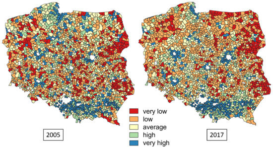
Figure 1.
Cohesion index values in 2005 and 2017 spatially for municipalities in Poland for five level clusters. Source: Own study.
In order to quantify the dynamics of change in the values of territorial cohesion indices over the years, in the next step, the indicators of the dynamics of change of the measures were also estimated and then juxtaposed in a two-dimensional space in order to examine the trends that developed in relation to these values (Figure 2). The slope of the index change dynamics cloud of observations confirms the relatively high decline in territorial cohesion during the period in question. The static values of the cohesion index in 2005 and 2017, as well as the dynamic changes in the index values in the years of analysis, were supplemented by the relationships between selected generic characteristics of municipalities and their spatial location.
At this stage, the level and dynamics of change in the CI were assessed in relation to the spatial location of the gmina, within one of seven macro-regions (NUTS 1), as well as the generic variable distinguishing between rural and urban-rural gminas (i.e., villages and small towns) and additionally supplemented by the population type of the gmina (the municipality population type was estimated using the following formula: Population (in thousands) in types and population types of municipalities: rural—smallest (<2.5), small (2.5–5), medium (5–10), large (10–15), largest (>15); urban-rural—smallest (<5), small (5–7.5), medium (7.5–15), large (15–30), largest (>30)) and the income group (defined as quartiles of the distribution of unit own income). By type, i.e., by municipality type, one can note the absence of a statistically significant difference between the average values in the group of rural and urban-rural municipalities. In the case of values for 2017, the average index value in both groups is similar (respectively: 0.6 and 0.66 in 2005 and 0.53 and 0.56 in 2017). After increasing the granularity of the data and also adding the dimension of the size of the municipality measured by the number of inhabitants to the analysis, it can be seen that despite the consistent decrease in the value of the index in most groups in subsequent years, a slight increase in cohesion in the period 2005–2017 was recorded in the group of the largest urban-rural and rural municipalities. Thus, we confirm that the size of the local administrative unit (gmina), measured by the population potential and spatial location of the gmina, significantly affect the obtained cohesion level. It may be pointed out that rural municipalities with the highest population potential were also characterized by a higher average level of cohesion than small and medium units. In regional terms, the highest cohesion indicator levels were noted in the southern macroregion while the lowest in the central and eastern macroregion.

Figure 2.
Dynamics of the territorial cohesion index in the studied group of municipalities in 2005–2017 in relation to the structural characteristics of the entities. Source: Own study.
The analysis of the cohesion level in groups of municipalities with respect to their income also makes it possible to identify the relationship between the level of a commune’s unit income, i.e., its financial standing, and the level and dynamics of the cohesion change. The average cohesion level in the group of gminas with a high income position (very large) exceeded the cohesion level by 1.5 times in the group of gminas with a low (small) level of the feature. Similarly, municipalities with a disadvantageous income situation were among those for which the cohesion regression was the highest and the most severe. Based on the above results, it may be concluded that the population and economic potential of a municipality as well as its spatial location are factors that influence the achieved territorial cohesion level and the dynamics and direction of change of its value in the period when the analysis was conducted.
3.3. Moran’s Autocorrelation Measure Assessment
The results of the estimation of autocorrelation measures indicate a progressive tendency to build spatial clusters in the case of the territorial CI, both in absolute terms and in the case of the dynamics of the phenomenon. The increase in the value of Moran’s global I statistic over the years 2005–2017 from 0.371 to 0.537, with an annual progression of 0.0093, indicates the strengthening of spatial dependencies. Based on the reported values we can read the tendency of greater polarization of the studied regions in space and greater spatial heterogeneity of phenomena in the case of territorial cohesion. The above observation is confirmed by the results of the estimation of the local measure of spatial autocorrelation (Ii), indicating a different shape of both the number and dynamics of clusters and hot-spots in individual years. In 2005, in the case of the measure of CI, 472 municipalities were surrounded by municipalities with similar values and formed the so-called clusters (high and low values), i.e., units grouped by similarity of characteristics, while in 2017, the number of such objects increased to 577, i.e., more than ¼ of the total population of the surveyed municipalities. This indicates a progressive polarisation of the territorial cohesion feature in the analysed years with a simultaneous decrease in the absolute level of the feature. In the analysed period, there was a significant decrease in the number of so-called hot-spots, i.e., areas grouping units with outliers.
3.4. Multinomial Ordered Logit Model Results
In the last stage of the analysis, a search for predictors was carried out, which, in principle, could explain the behaviour of the CIs of the analysed municipalities. For this purpose, on the basis of literature sources, a set of indicators describing various aspects of the activity of municipalities was identified, in terms of physical characteristics, size, and financial strength and economic efficiency (Table 5).
Table 5.
Independent variables used to construct the multinomial logit model.
The selection of explanatory variables was the result of literature studies on factors affecting the level of territorial cohesion, among others, by Kluza [54] and Spychała [55,56]. It is indicated that the level of territorial cohesion and the ability to increase it is determined by a number of endogenous characteristics of the local government unit and can be strengthened by exogenous support tools (external funds).
In the case of endogenous characteristics, objective characteristics are important, including spatial location, including proximity or peripherality to regional centres, which determines the so-called rent of location. The physical size of the local administrative unit measured by area was also taken into account, which determines, among other things, the degree of dispersion of the settlement network, which affects the cost intensity and economic viability of developing elements of technical infrastructure (mainly transmission networks) and data on social infrastructure (educational, health care, and cultural institutions).
The type of municipality and its size with respect to population resources has a direct bearing on its economic resources, particularly the amount of annual revenues, which is the result of the subsidy algorithm allocating tax revenues from personal and corporate taxes according to the population key. In turn, the administrative unit’s own financial resources determine its ability to undertake investment activity, and indirectly, they are also a factor affecting the possibility of obtaining external financing, both repayable (liabilities) and non-repayable (primarily in the form of aid funds from the European Union). In both cases, a gmina’s own financial strength is a factor that determines its creditworthiness and its ability to obtain aid funds (due to the necessity to make an own contribution). Therefore, in this analysis, statistics describing the ability of an administrative unit (commune) to generate added value (operating surplus, self-financing rate) as well as the size of external financial resources and the intensity of support from European Union funds were used. In this case, it was assumed that the achievement of territorial cohesion should be particularly influenced by the resources of the cohesion funds distributed under the operational programmes implemented in the regions; hence, this category of funds was separated for the programming period 2007–2013 both in relation to the financial value of assistance, as well as in relation to the number of projects implemented in the area of a given territorial unit (gmina). Given that support for cohesion is also contained in a number of measures in the field of rural development, the total value of support in the period 2007–2013, both as shares and in absolute terms, was also taken into account as a predictor of the level of cohesion. In addition to this, the value of unit support for the initial years of the next programming period (2014–2020) was included in the analysis [57].
The quantitative approach used in the analysis included regression calculus in the form of a multinomial logit ordered model. In the case of the multinomial logit model, the estimation of parameters and values of explanatory variables allows determination of the probability of the belonging of each observation to particular categories of the explained variable and then on their basis to assign each observation to the predicted category. The maximum likelihood principle is used here, according to which the observation is assigned to the category for which the probability of the belonging of the observation is the highest. Preliminary analysis of the correlation coefficients showed a relatively low level of correlation between explanatory variables, suggesting no threat of collinearity (Table 6).
Table 6.
Pearson correlation coefficients for continuous explanatory variables describing the level of territorial cohesion index.
The next step was to estimate the multinomial ordered logit with the dependent variable—the value of territorial CI in 2017 divided into 5 groups. The actual values of the territorial cohesion index were assigned to each value group using the mean value and standard deviation in the population, according to the scheme shown in Table 1. The explanatory variables were assigned to eight generic groups defining the relative position of the municipality in the population in terms of human resources and the size of the area, and physical characteristics—the area of the municipality and its location in relation to the central centre of the region, the level of civic involvement, measured by the propensity to participate in local elections, the financial strength of the entity in terms of the ability to generate own income, operating surplus, and debt level, the intensity of use of EU support funds in the financial perspective 2007–2013 and in the initial years of the financial perspective 2014–2020, the generic and population type of the municipality, and the spatial location defined by belonging to the relevant macro-region. Table 7 gives the results of model estimation. Positive (or negative) signs of estimated parameters for explanatory variables mean that as the value of a given variable increases (decreases), the probability of classifying an object to a higher ordinal category. In case of ranking variables (describing place of the gmina in the classification on the basis of the population and area criterion), the probability distribution has a logical and ordered character. In the case of the population ranking, as the size of the gmina measured by its place in the ranking decreases, the chance of assigning it to the lowest category of the cohesion index increases. In the case of the area ranking, this relationship is reversed. In the case of variables describing the financial condition of the gmina (the self-financing ratio and the financial surplus measure), the distribution of probabilities of entering particular categories of the index indicates a significant association between their maximisation and achieving a higher level of cohesion (the probability of being assigned to the highest category increases as the value of indicators increases). On the other hand, the distribution of variables describing the size and structure of the municipality’s indebtedness does not allow for unequivocal conclusions as to the direction of the relationship with the explained variable. Interpretation of the results indicates a sharp increase in the probability of being assigned to the lowest cohesion category along with an increase in the distance between a gmina and an NUTS 2 capital city as well as the size of the gmina measured by area. The highest CI values were recorded for gminas situated in a belt directly adjacent to the regional centre and to a lesser extent for gminas situated in the “second circle”, i.e., a farther belt surrounding the centre. A location in a belt directly adjacent to the region’s centre statistically significantly increases the chances of finding oneself in the highest cohesion cohorts. In the case of municipalities located farther away, this effect is also positive and statistically significant, although of lesser strength than in the case of the closer group. On the basis of the estimated values, it may be concluded that the range of break-even distances from the centre, beyond which a sharp decline in the probability of achieving high cohesion occurs, is in Poland approximately 50–60 km and is derived from the transport accessibility of the local government unit measured by the time of commuting to the centre (city) [58]. In the case of municipality revenues from the European Union funds, the lack of significance of a number of variables in this category when explaining the cohesion index level indicates that there is no unambiguous relationship between the discussed variables and the CI.
Table 7.
Results of estimation of multinomial ordered logit with dependent variable—value of territorial CI in 2017 by 5 groups.
It is important to point out the positive but statistically insignificant impact on the cohesion of measures from regional operational programs, which are the most diverse and cover the widest range of activities aimed at developing technical, social, and educational infrastructure, supporting innovation and technological development, the development of entrepreneurship, but also low-carbon economy, environmental protection and natural resources, modern transport, or the development of the labour market and social inclusion [12]. However, this study confirms that there is a limit to the share of EU funds in the revenues of the municipality, beyond which the positive impact on cohesion will stop. This limit is, according to other studies, around 10% of the share of income [59,60]. Such a result clearly favours larger units with more resources, especially financial, allowing for off-set of increased inflow of funds and more efficient use of them.
3.5. Marginal Effects Analysis for Multinomial Logit Estimation Results
A marginal effects analysis (Table 8) showed the probability of finding oneself in a given CI level group depending on the intensity of the use of funds from the regional operational programs, both in terms of amounts (as a total amount per capita) and in terms of quantities in relation to the number of projects implemented in the area of a given gmina. The CI value decreases with increasing dependence between the size of gmina revenues and the size of the EU funds received while the probability of achieving low cohesion increases with an increase in the share of aid funds in revenues. This clearly indicates that there are limits to the positive impact of revenues from the EU on the possibility of achieving a high level of cohesion, with limited own resources generated by the administrative unit (gmina).
Table 8.
Marginal effects for multinomial ordered logit model with dependent variable—territorial cohesion index value in 2017 divided into 5 groups.
In the case of generic variables, according to the marginal effects calculus, assignment to the category of rural gminas lowers the probability of being in the lowest (very low) cohesion group by 5% and at the same time increases the probability of being classified in the highest (very high) cohesion category by 5%. A positive relationship with the dependent variable indicating an increase in territorial cohesion ceteris paribus was found in the case of the variables: place in the national ranking by population, participation in local elections, own income, both in relative and absolute terms (per head), operating surplus, and unit value of liabilities. The positive value of the regression coefficient was also found for all variables assigned to the sub-categories of the intensity of financial support from the EU and the type and population features.
4. Conclusions
Studies on the level and dynamics of territorial cohesion in 2005–2017 for municipalities in rural areas in Poland, determined by the degree of demographic, economic, infrastructural, and environmental development, have shown that in the development of rural space, there are processes of relatively strong polarization. The gap between gminas with a very low and very high cohesion level increased, which testifies to the deepening of inequalities between gminas. This reflects persistent trends in the development of rural space. Demographic, economic, and infrastructure development opportunities, and with them the level of territorial cohesion achieved, depend on the characteristics of the administrative unit under analysis, including in particular its population and its location in relation to larger urbanisation centres. Development indicators are much lower for gminas with a smaller number of inhabitants and those located peripherally in relation to a large settlement centre, irrespective of other characteristics taken into account in the assessment of a given administrative unit. The poles of demographic, economic, infrastructural, and environmental development are formed by gminas with a larger number of inhabitants.
The analysis revealed that there has been a decline in global cohesion as measured by the level of the aggregate cohesion index. There are clear differences in terms of the level of territorial cohesion in individual regions in Poland, but they are partly derived from endogenous factors related to the rent of location and population resources, which cannot easily be modified. In particular, big agglomerations and large cities are the strongest centres of development and technology diffusion in their regions [61]. Among partial determinants, which result from the analysis of unaggregated indicators, it should be indicated that unfavourable demographic tendencies connected with progressing depopulation of rural areas and an unfavourable population structure connected with the share of particular age groups and the size of an economically active population constitute a particular threat for the current and future cohesion level. The change of demographic trends, in contrast to infrastructural, economic, and environmental elements, is a slow and long-term process [20,62]. From the perspective of the adopted characteristics, between 2005 and 2017, there was an increase in the differentiation between municipalities in the regions, i.e., a decrease in the degree of internal cohesion in NUTS 2 regions. The intensity of the process of catching up of municipalities with a higher level of development and cohesion level by municipalities with a lower level is low, which may indicate that on a local scale, territorial cohesion is reached too slowly. This is a particularly worrying symptom in a country that is a beneficiary of cohesion policy, since its funds are spent precisely on reducing disparities between regions and within regions, i.e., among local units (gminas) in the region.
The observation of socio-economic phenomena in 2005–2017 confirms that specific groups of municipalities require a separate cohesion policy, which would create conditions for better use of existing and potential local resources in accordance with the strategic objectives of the region [33]. The implementation of the current ‘polarisation-diffusion’ model carries the risk of deepening disparities in terms of economic and social cohesion [63]. Differences between municipalities or regions are the result of many socio-economic factors and relations between them. They are caused mainly by the polycentric nature of the spatial structure and metropolisation processes, i.e., the creation of distinct growth poles around large cities [32]. As a result, it seems necessary to increase the role of regional and subregional centres in favour of areas lying outside their direct influence. In the case of peripheral areas, greater support for the regional policy with additional special support instruments or interventions is required. They should be spatially differentiated and adapted to the specific conditions existing in the region, or even in the commune, which should reduce the effects of spatial polarisation of development. It is necessary to develop a rational concept of a network of settlement units where infrastructure facilities should be located and to take care of their road and communication accessibility. This may ensure an efficient system of providing public services, which is related to improvement of the quality of life in rural areas. Undertaking activities towards further deconcentration of financial instruments of gminas gives them a chance for a comprehensive grasp of local development factors and implementation of activities within the framework of climate policy taking into account external instruments. A more flexible approach to credit limits of individual municipalities should be advocated. This could, on the one hand, limit the temptation of over-indebtedness of economically weak entities and, on the other hand, weaken unnecessary restrictions that constrain municipalities capable of intensive indebtedness.
The analytical approach presented in this paper was carried out at the level of delimitation commonly used in Europe; therefore, the logic and techniques of the analysis provide an opportunity to incorporate this approach into the toolkit for national and local evidence-based policy making.
Author Contributions
Conceptualization, M.G. and P.C.; methodology, M.G. and P.C.; software, M.G.; validation, M.G.; formal analysis, M.G. and P.C.; investigation, M.G. and P.C.; data curation, M.G.; writing—original draft preparation, M.G. and P.C.; writing—review and editing, P.C. and M.G.; visualization, M.G.; supervision, P.C. and M.G. All authors have read and agreed to the published version of the manuscript.
Funding
This research received no external funding.
Institutional Review Board Statement
Not applicable.
Informed Consent Statement
Not applicable.
Data Availability Statement
Data used in the paper are from Local Data Bank of the Statistics Poland, available: https://bdl.stat.gov.pl/BDLS/pages/Home.aspx (accessed on 1 June 2021).
Conflicts of Interest
The authors declare no conflict of interest.
References
- Van Well, L. Conceptualizing the logics of territorial cohesion. Eur. Plan. Stud. 2012, 20, 1549–1567. [Google Scholar] [CrossRef]
- Davoudi, S. Understanding territorial cohesion. Plan. Pract. Res. 2005, 20, 433–441. [Google Scholar] [CrossRef]
- Molle, W. European Cohesion Policy; Routledge: London, UK, 2007. [Google Scholar]
- Ryszkiewicz, A. Od Konwergencji Do Spójności i Efektywności: Podstawy Teoretyczne Polityki Spójności Gospodarczej, Społecznej i Terytorialnej Unii Europejskiej; Szkoła Główna Handlowa-Oficyna Wydawnicza: Warszawa, Poland, 2013. [Google Scholar]
- Battaini-Dragoni, G.; Dominioni, S. The Council of Europe’s Strategy for Social Cohesion. 2003. Available online: http://www.socsc.hku.hk/cosc/Full%20paper/BATTAINI-DRAGONI%20Gabriella (accessed on 22 August 2021).
- Keck, W.; Krause, P. How Does EU Enlargement Affect Social Cohesion? DIW Discussion Papers: Berlin, Germany, 2006. [Google Scholar]
- Kalinowski, S.; Rosa, A. Sustainable Development and the Problems of Rural Poverty and Social Exclusion in the EU Countries. Eur. Res. Stud. J. 2021, 24, 438–463. [Google Scholar] [CrossRef]
- Faludi, A. Territorial cohesion and subsidiarity under the European Union treaties: A critique of the ‘territorialism’underlying. Reg. Stud. 2013, 47, 1594–1606. [Google Scholar] [CrossRef]
- Szlachta, J. Territorialisation as a Challenge for Development Policy–European Perspective. Studia KPZK 2018, 184, 10–19. [Google Scholar]
- Fratesi, U.; Wishlade, F.G. The impact of European Cohesion Policy in different contexts. Reg. Stud. 2017, 51, 817–821. [Google Scholar] [CrossRef]
- Gagliardi, L.; Percoco, M. The impact of European Cohesion Policy in urban and rural regions. Reg. Stud. 2017, 51, 857–868. [Google Scholar] [CrossRef]
- Chmieliński, P.; Gospodarowicz, M. A Regional Approach to Rural Development? Regional and Rural Programmes in Poland 2007–2015. Wieś Rol. 2018, 4, 181–198. [Google Scholar] [CrossRef]
- Bachtler, J.; Downes, R.; Gorzelak, G. Transition, cohesion and regional policy in Central and Eastern Europe: Conclusions. In Transition, Cohesion and Regional Policy in Central and Eastern Europe; Routledge: London, UK, 2019; pp. 355–378. [Google Scholar]
- Balz, V.E.; Nadin, V.; Zonneveld, W.; Piskorek, K.; Georgieva, N.; den Hoed, A.; Unceta, P.M.; Hermansons, Z.; Daly, G. Cross-fertilisation of cohesion policy and spatial planning. ESPON Policy Brief: Luxembourg 2021. Available online: https://research.tudelft.nl/en/publications/cross-fertilisation-of-cohesion-policy-and-spatial-planning-espon/ (accessed on 22 August 2021).
- Shaping New Policies in Specific Types of Territories in Europe: Islands, Mountains, Sparsely Populated and Coastal Regions. 2017. Available online: https://www.espon.eu/topics-policy/publications/policy-briefs/shaping-new-policies-specific-types-territories-europe (accessed on 22 August 2021).
- Lenschow, A. Dynamics in a multilevel polity: Greening the European Union Regional and cohesion funds. In Environmental Policy Integration; Routledge: London, UK, 2012; pp. 203–225. [Google Scholar]
- Gorzelak, G. Social and Economic Development in Central and Eastern Europe: Stability and Change after 1990; Routledge: London, UK, 2019. [Google Scholar]
- Zaucha, J.; Böhme, K. Measuring territorial cohesion is not a mission impossible. Eur. Plan. Stud. 2020, 28, 627–649. [Google Scholar] [CrossRef]
- Matsumoto, A.; Merlone, U.; Szidarovszky, F. Some notes on applying the Herfindahl–Hirschman Index. Appl. Econ. Lett. 2012, 19, 181–184. [Google Scholar] [CrossRef]
- Prezioso, M. Cohesion policy: Methodology and indicators towards common approach. Rom. J. Reg. Sci. 2008, 2, 1–32. [Google Scholar]
- Medeiros, E. Territorial Cohesion: A Conceptual Analysis; Institute of Geography and Spatial Planning (IGOT) Alameda da Universidade: Lizbona, Portugal, 2011; Available online: http://ww3.fl.ul.pt/pessoais/Eduardo_Medeiros/docs/PUB_PAP_EM_Territorial_Cohesion.pdf (accessed on 22 August 2021).
- Komornicki, T.; Ciołek, D. Territorial capital in Poland. In Territorial Cohesion: A Missing Link between Economic Growth and Welfare. Lessons from the Baltic Tiger; Bradley, J., Zaucha, J., Eds.; University of Gdańsk: Gdańsk, Poland, 2017; pp. 23–48. [Google Scholar]
- Bencardino, F.; Cresta, A.; Greco, I. Territorial Cohesion Concept and Measuring: Territorial Impact Assessment of Regional Policies. The Case of the Campania Region. Boll. Della Soc. Geogr. Ital. 2019, 2, 49–62. [Google Scholar]
- Vogelaar, T.W. Approximation of the Laws of Member States under the Treaty of Rome, The. Common Mark. L. Rev. 1975, 12, 211. [Google Scholar]
- Schön, K.P. Territorial cohesion–Current views of the commission and the member states of the European Union. In German Annual of Spatial Research and Policy 2009; Springer: Berlin/Heidelberg, Germany, 2009; pp. 7–17. [Google Scholar]
- Gospodarowicz, M. Social and technical infrastructure development of municipalities (gminas) in Poland. Stud. Agric. Econ. 2015, 117, 147–154. [Google Scholar] [CrossRef][Green Version]
- Di Comite, F.; Lecca, P.; Monfort, P.; Persyn, D.; Piculescu, V. The Impact of Cohesion Policy 2007–2015 in EU Regions: Simulations with the RHOMOLO Interregional Dynamic General Equilibrium Model; JRC Working Papers on Territorial Modelling and Analysis: Sevilla, Spain, 2018. [Google Scholar]
- Piattoni, S.; Polverari, L. Handbook on Cohesion Policy in the EU.; Edward Elgar Publishing: Cheltenham, UK, 2016. [Google Scholar]
- Rural Areas in Poland in 2018; GUS: Warsaw, Poland, 2018.
- Zegar, J.; Zrównoważenie Polskiego Rolnictwa. Powszechny Spis Rolny 2010 (Sustainability of Polish agriculture. In 2010 Agricultural Census); 2013. Available online: https://stat.gov.pl/obszary-tematyczne/rolnictwo-lesnictwo/psr-2010/powszechny-spis-rolny-2010-zrownowazenie-polskiego-rolnictwa,11,1.html (accessed on 22 September 2021).
- Baldersheim, H.; Rose, L. Territorial Choice: The Politics of Boundaries and Borders; Springer: Berlin/Heidelberg, Germany, 2010. [Google Scholar]
- Copus, A.K.; Shucksmith, M.; Dax, T.; Meredith, D. Cohesion Policy for rural areas after 2013. A rationale derived from the EDORA project (European Development Opportunities in Rural Areas)–ESPON 2013 Project 2013/1/2. Stud. Agric. Econ. 2011, 113, 121–132. [Google Scholar] [CrossRef]
- Dąbrowski, M. EU cohesion policy, horizontal partnership and the patterns of sub-national governance: Insights from Central and Eastern Europe. Eur. Urban Reg. Stud. 2014, 21, 364–383. [Google Scholar] [CrossRef]
- Sánchez-Zamora, P.; Gallardo-Cobos, R. Territorial Cohesion in Rural Areas: An Analysis of Determinants in the Post-Economic Crisis Context. Sustainability 2020, 12, 3816. [Google Scholar] [CrossRef]
- Sanchez-Zamora, P.; Gallardo-Cobos, R.; Romero-Huertas, C. Assessing the determinants of territorial cohesion: Evidence from Colombian departments. Geoforum 2017, 87, 48–61. [Google Scholar] [CrossRef]
- Reig-Martínez, E.; Gómez-Limón, J.A.; Picazo-Tadeo, A.J. Ranking farms with a composite indicator of sustainability. Agric. Econ. 2011, 42, 561–575. [Google Scholar] [CrossRef]
- Adamowicz, M.; Smarzewska, A. Model oraz mierniki trwałego i zrównoważonego rozwoju obszarów wiejskich w ujęciu lokalnym. Zesz. Nauk. SGGW Polityki Eur. Finans. Mark. 2009, 1, 251–269. [Google Scholar]
- Jańczuk, L. Determinants of the socio-economic development of regions in Poland. Rocz. Nauk Społecznych 2013, 5, 121–132. [Google Scholar]
- Hellwig, Z. Application of the Taxonomic Method to the Countries Typology according to their Level of Development and the Structure of Resources and Qualified Staff. Przegląd Stat. 1968, 4, 307–326. [Google Scholar]
- Bąk, A. Linear ordering of objects using Hellwig and TOPSIS methods-a comparative analysis. Res. Pap. Wrocław Univ. Econ. 2016, 426, 22–31. [Google Scholar]
- Charnes, A.; Cooper, W.W.; Rhodes, E. Measuring the efficiency of decision making units. Eur. J. Oper. Res. 1978, 2, 429–444. [Google Scholar] [CrossRef]
- Medeiros, E. Territorial cohesion: An EU concept. Eur. J. Spat. Dev. 2016, 60, 1–30. [Google Scholar]
- Stanny, M. Poziom rozwoju społeczno-gospodarczego obszarów wiejskich w Polsce–pomiar zjawiska złożonego. In Rozwój Wsi i Rolnictwa w Polsce. Aspekty Przestrzenne i Regionalne; IRWiR PAN: Warszawa, Poland, 2012. [Google Scholar]
- Parysek, J.J. Rozwój społeczno-gospodarczy oraz czynniki i uwarunkowania rozwoju. Studia KPZK 2018, 183, 37–56. [Google Scholar]
- Adamowicz, M.P. Janulewicz. The use of multidimensional methods in determining the competitive position of communes on the example of Lublin voivodeship. Quant. Methods Econ. Res. 2012, 12, 17–28. [Google Scholar]
- González, A.; Daly, G.; Pinch, P.; Adams, N.; Valtenbergs, V.; Burns, M.C.; Johannesson, H. Indicators for Spatial Planning and Territorial Cohesion: Stakeholder-Driven Selection Approach for Improving Usability at Regional and Local Levels. Reg. Stud. 2015, 49, 1588–1602. [Google Scholar] [CrossRef]
- Jakubowski, A. Convergence or Divergence? Multidimensional Analysis of Regional Development in the New European Union Member States. Barom. Regionalny. Anal. Progn. 2018, 16, 31–40. [Google Scholar]
- Moran, P.A. Notes on continuous stochastic phenomena. Biometrika 1950, 37, 17–23. [Google Scholar] [CrossRef]
- Anselin, L. Local indicators of spatial association—LISA. Geogr. Anal. 1995, 27, 93–115. [Google Scholar] [CrossRef]
- Boes, S.; Winkelmann, R. Ordered response models. Allg. Stat. Arch. 2006, 90, 167–181. [Google Scholar]
- Schultz, T.W. Investment in human capital. Am. Econ. Rev. 1961, 51, 1–17. [Google Scholar]
- Chmieliński, P.; Chmielewska, B. Social changes in rural areas: Incomes and expenditures of rural households. Eкoнoмикa пoљoпpивpeдe 2015, 62, 907–921. [Google Scholar] [CrossRef]
- World Population Prospects: The 2017 Revision, Key Findings and Advance Tables; United Nations, Department of Economic and Social Affairs, Population Division: New York, NY, USA, 2017.
- Kluza, K. Socio-economic disparities between rural boroughs as a function of their peripheral location. Pr. Nauk. Uniw. Ekon. We Wrocławiu 2019, 63, 37–48. [Google Scholar] [CrossRef]
- Spychała, M. Zróżnicowanie przestrzenne absorpcji funduszy unijnych perspektywy finansowej 2007–2013 a zmiany poziomu wzrostu gospodarczego województw w Polsce. Nierówności Społeczne Wzrost Gospod. 2017, 49, 348–358. [Google Scholar] [CrossRef]
- Spychała, M. The absorption of EU funds and the socio-economic development in the subregional dimension in Poland. Pr. Nauk. Uniw. Ekon. We Wrocławiu 2020, 64, 78–91. [Google Scholar] [CrossRef]
- Rakowska, J.; Wojciechowska, E. Znaczenie PROW 2007–2013 jako instrumentu wsparcia inwestycji samorządów gmin wiejskich powiatu pułtuskiego. Roczniki SERiA 2017, XIX/5, 179–184. [Google Scholar]
- Kruszyna, M.; Śleszyński, P.; Rychlewski, J. Dependencies between demographic urbanization and the agglomeration road traffic volumes: Evidence from Poland. Land 2021, 10, 47. [Google Scholar] [CrossRef]
- Dall’Erba, S.; Fang, F. Meta-analysis of the impact of European Union Structural Funds on regional growth. Reg. Stud. 2017, 51, 822–832. [Google Scholar] [CrossRef]
- Dubownik, A.; Rudnicki, R.; Wiśniewski, Ł. Fundusze Unii Europejskiej jako czynnik rozwoju obszarów wiejskich w województwie kujawsko-pomorskim (lata 2007–2013)= European Union funds as a factor in the development of rural areas in Kujawsko-Pomorskie province (in 2007–2013 period). Studia Obsz. Wiej. 2017, 47, 55–75. [Google Scholar] [CrossRef]
- Frederickson, H.G.; Johnson, G.A.; Wood, C. The changing structure of American cities: A study of the diffusion of innovation. Public Adm. Rev. 2004, 64, 320–330. [Google Scholar] [CrossRef]
- Tijanic, L.; Gombar, D. Managing Regional Demographic Polarisation in Croatia-the Role of Cohesion Policy. Econ. Soc. Dev. Book Proc. 2019, pp. 477–487. Available online: https://www.esd-conference.com/upload/book_of_abstracts/Book_of_Abstracts_esdRabat2019_Online.pdf (accessed on 22 September 2021).
- Komorowski, Ł.; Mróz, A.; Stanny, M. The Spatial Pattern of the Absorption of Cohesion Policy Funds in Polish Rural Areas. Land 2021, 10, 26. [Google Scholar] [CrossRef]
Publisher’s Note: MDPI stays neutral with regard to jurisdictional claims in published maps and institutional affiliations. |
© 2021 by the authors. Licensee MDPI, Basel, Switzerland. This article is an open access article distributed under the terms and conditions of the Creative Commons Attribution (CC BY) license (https://creativecommons.org/licenses/by/4.0/).