A Robust Fractional-Order PID Controller Based Load Frequency Control Using Modified Hunger Games Search Optimizer

Abstract

In this article, a recent modified meta-heuristic optimizer named the modified hunger games search optimizer (MHGS) is developed to determine the optimal parameters of a fractional-order proportional integral derivative (FOPID) based load frequency controller (LFC). As an interconnected system’s operation requires maintaining the tie-line power and frequency at their described values without permitting deviations in them, an enhanced optimizer is developed to identify the controllers’ parameters efficiently and rapidly. Therefore, the non-uniform mutation operator is proposed to strengthen the diversity of the solutions and discover the search landscape of the basic hunger games search optimizer (HGS), aiming to provide a reliable approach. The considered fitness function is the integral time absolute error (ITAE) comprising the deviations in tie-line power and frequencies. The analysis is implemented in two networks: the 1st network comprises a photovoltaic (PV) plant connected to the thermal plant, and the 2nd network has four connected plants, which are PV, wind turbine (WT), and 2 thermal units with generation rate constraints and governor dead-band. Two different load disturbances are imposed for two studied systems: static and dynamic. The results of the proposed approach of MHGS are compared with the marine predators algorithm (MPA), artificial ecosystem based optimization (AEO), equilibrium optimizer (EO), and Runge–Kutta based optimizer (RUN), as well as movable damped wave algorithm (DMV) results. Moreover, the performance specifications of the time responses of frequencies and tie-line powers’ violations comprising rise time, settling time, minimum/maximum setting values, overshoot, undershoot, and the peak level besides its duration are calculated. The proposed MHGS shows its reliability in providing the most efficient values for the FOPID controllers’ parameters that achieve the lowest fitness of 0.89726 in a rapid decaying. Moreover, the MHGS based system becomes stable the most quickly as it has the shortest settling time and is well constructed as it has the smallest peak, overshoots at early times, and then the system becomes steady. The results confirmed the competence of the proposed MHGS in designing efficient FOPID-LFC controllers that guarantee reliable operation in case of load disturbances.

1. Introduction

In today’s era, the traditional grids are considered less reliable and unable to meet the requirement of supplying excessive electrical power to consumers. The main reason is the depletion of fossil fuels which has occurred at a much higher rate in the last few decades. Thereby, with currently expanding energy utilization, the power industry is confronted with introducing new power generation plants, transmission, and distribution networks. Renewable energy based power plants and distributed generation (DG) are trendy and suitable options to conquer this issue [1,2].

In addition, to furnish a stable power supply to the consumers and to meet the required energy demand, the present power system has been changed from a conventional larger power grid to a multi-area interconnected power system [3]. The coordination and advancement of conventional interconnection can significantly ameliorate the stability, economy, and reliability of the grid. In this manner, the regional interconnected power grid is the fundamental pattern of the present power grid improvement. In any case, in crisis conditions, when enormous variations are occurring, they become detached from the main grid to supply the emergency loads. In these conditions, there are variations in solar irradiation, wind speed, and load damping issues of frequency variations known as load frequency control (LFC) [4]. Continuous frequency variations in power networks lead to serious harm to frequency-sensitive devices, failure in the operation of protection devices, and overload of transmission lines. On the other hand, an increase in the number of renewable distributed generations (DGs) in the power network also increases irregular power output. This results in complex frequency control. Therefore, to maintain the reliable and stable power network implementation of an efficient LFC technique is obligatory.

Therefore, the stability of a power network relies upon how great the power generation coordinates with the complete demand are, along with losses in the system through any load fluctuations. In this regard, the LFC of a power system network is a critical part of power quality. The LFC targets maintain zero steady-state errors for region frequencies and tie-line power streams between the interconnected regions and also manages the symmetry between the power consumption and generation [5]. In addition, the main idea behind LFC is to manage the frequency of every area inside the specified limits even in case of load change conditions and large variations occurring from integrated renewable energy resources (RESs) [6]. From the literature, it is found that, for multi-area power networks, distributed LFC innovations are highly encouraging when compared to their centralized peers.

To achieve the above-specified targets, numerous researchers and communities have worked on LFC in the past few years. Numerous control strategies have been implemented in the past for the LFC issues. From the existing literature and various control methods proposed by the researchers, the design of the controller can be classified into two types. These are (1) control techniques depending on traditional methods and (2) those depending on meta-heuristic or soft computing techniques. Proportional-integral-derivative (PID) controllers have been widely used by numerous researchers and in industry for the application of LFC due to their wide range of features, namely, simplicity of tuning and structure, no need for any expertise-specific requirements, reliable operation, and  good concordance between cost and performance. Classical control techniques concentrating on proportional-integral-derivative (PID) controllers [7], with consideration of robustness and sensitivity to measurements of noise for PID-LFC, have been proposed by the authors in [8], as well as sliding mode control (SMC) [9].

The integral control technique is the one extensively used for LFC. However, in this method, the gain of the integral controller is tuned in offline mode. Therefore, it results in poor dynamic performance in case of system changes and load fluctuations. To resolve the issue of offline tuning, fixed parameter PI controllers have been introduced in [10]. Ali Kazemy et al. [11] used a combination of conventional PC controllers and mode-dependent state feedback controllers for LFC. In this work, the authors considered an event-triggered mechanism to minimize unessential data transfer along with the network. In [12], the authors introduced virtual inertia of a wind generator to manage load frequency and damping oscillations in interconnection lines. Virtual wind inertia has been extensively analyzed to control the frequency. As the wind plants are connected to the grid via converters, they can act rapidly to furnish LFC with fast dynamics. Due to the extensive intelligent control, the best outcomes were attained with the conventional LFC.

In [13], the authors proposed a decentralized biased PI dual-mode controller with consideration of governor dead-band and generation rate constraint non-linearities for LFC. Tarek Hassan et al. [14] introduced a balloon effect modification to the Jaya algorithm under both parameter and load variations. The modified Jaya technique was applied on a new objective function to control the online system problems [14]. This technique was evaluated by those authors by considering the frequency variations that occurred due to variations in the system parameters and step demand loads [14]. The effectiveness of the proposed technique is correlated with the effectiveness of regular integral controllers and classical Jaya control techniques. A novel adaptive SMC was proposed in [15], and it achieved a better performance than classical SMC. In [16], Arivoli et al. designed a PI controller via craziness particle swarm optimization (CPSO) based integral square error (CPSOISE), multi-objective based CPSO, and CPSO based apex stability verge for LFC. Yogendra et al. [17] developed a bacterial foraging optimization (BFOA) based fuzzy PI/PID controller for automatic generation control (AGC) of a two-area network. The excellence of the proposed technique was compared to the results of firefly, particle swarm (PSO), hybrid BFOA-PSO based PI controllers, and PSO and pattern search (PS) optimized fuzzy PI controllers. Sensitivity analysis was executed to investigate the robustness of all designed controllers under study. Similarly, in [18], a hybrid version of differential evolution and pattern search (DE-PS) was considered to optimize the modified ID controller for the objective of LFC. Fractional order type 2 fuzzy based on the Levenberg–Marquardt algorithm (LMA) was proposed to simulate LFC by the authors in [19]. In this approach, FOPID is used instead of traditional PID due to a high number of adjustable parameters, robustness, and being faster than other techniques. The gradient descent algorithm (GDA) was used in [20] to train and the optimization approach was applied to the controller. However, from the results of GDA, it is observed that the shortcomings of the method are lower speed in finding the training rate and high sensitivity to initial conditions. Bhuvnesh Khokhar et al. [21] proposed a two-dimensional sine logistic map with a chaotic sine cosine algorithm (2D-SLCSCA) for tuning the PID controller of an islanded microgrid for LFC. The proposed algorithm was developed with the aim of improving the search capability and convergence speed of the algorithm with the utilization of extensive 2D chaotic-like retaining a broader chaotic range and ergodic. The efficacy of the developed technique has been compared with PSO, grey wolf optimizer (GWO), salp swarm algorithm (ISSA), 2D Lozi map, and Henon map based chaotic SCA under diversified load fluctuations. Using the 2D-SLCSCA technique, the authors enhanced the frequency response percentage by 96.51% during objective function, 78.89% during peak overshoot, and 78.86%, during undershoot conditions as compared to their counterparts.

With the attractive features ofthe dragonfly algorithm (DA) such as easy modification, hybridization, and utilizable in different applications, the authors in [22] proposed a quasi-oppositional dragonfly algorithm (QODA) to design a PID controller which is correlated with the performance of a conventional PID controller for three- and two-area interconnected power systems. Oshnoei et al. [23] proposed a hybrid controller based on two degrees of freedom (2DOF) with a combination of a fractional-order PID and tilt integral derivative controller. This controller has been successfully employed for a two-area interconnected power system network comprising a wind turbine (WT) and redox flow battery. To assess the suitability of the proposed controller for real-time applications, examinations in two areas and the New England 39 bus power system have been taken into account. In [24], a 2DOF-FOPID is proposed using a quasi-oppositional based salp swarm algorithm to tune the gains of the controller. In addition, some other meta-heuristic based algorithms were implemented for the LFC, such as grey wolf optimizer (GWO) [25], artificial bee colony (ABC) [26], ant lion optimizer (ALO) [27], human brain emotional learning algorithm [28], binary bat algorithm (BBA) [29], marine predators algorithm [30], and differential evolution (DE) [31].

The hybrid or improved versions of algorithms proposed for the same are improved ant colony optimization (ICMPACO) [32], adaptive learning strategy based PSO (ALPSO) [33], hybrid algorithm combining firefly and PSO (HFPSO) [34], improved salp swarm algorithm (ISSA) [35], and hybrid differential evolution and biogeography based optimization (DE/BBO) approach [36].

From the analysis on various techniques, it is found that fractional-order controllers (FOCs) are the most efficient approach as they are impervious to variations in the operating circumstances and network parameters [37]. Therefore, FOCs have attracted many researchers to incorporate them for effective LFC. In [38], Fuzzy logic based fractional-order PID (FOPID) has been utilized as a secondary frequency controller of hydro-thermal power systems. In this work, the authors considered the bacterial foraging algorithm (BFA) to find the optimal parameters of the controller. Zamani et al. employed a gases’ Brownian movement optimization algorithm to tune the parameters of the FOPID controller to relieve the tie-line power flow and frequency deviations in a two-region power network [39]. The other type of FOC and FOPID controller, named the tilt integral derivative (TID) controller, has been proposed via improved PSO to enhance the system performance even under typical conditions [37,40]. Similarly, the same TID is tuned by the water cycle algorithm in [41]. A multi-objective optimization model for both frequency and voltage control is proposed in [42]. The FOPID controller via a sine-cosine optimization for doubly-fed induction generation with the aim of frequency and tie-line power violations is proposed in [43]. A flower pollination based FOPID was developed for a two-area power network of an electric vehicle to improve the capability of AGC [44].

Notwithstanding the benefits of the existing control techniques, it is noteworthy to mention the criticalities of incorporating these techniques. These are, namely, that adaptive techniques are complex, online parameter tuning, and that these techniques require an absolute system model. The classical Jaya algorithm completely depends on the plant’s transfer function and assumes a disturbance-free system. This is the major limitation of the technique where the system encounters disturbances [14]. The listed control techniques reported in the literature, such as adaptive controllers, SMC, and fractional-order controllers, demonstrated an effective performance when employed in the dynamic systems’ control schemes. However, they encounter various restrictions, namely, design complexity, high computation burden and time, and requirement for expertise to tune the control parameters, and involve higher costs than conventional controllers [45]. The traditional controllers are less costly and simple in design, but these controllers fail when the system undergoes non-linearities and show high sensitivity towards small changes in system parameters [46]. In addition, most of the proposed meta-heuristic algorithms may become trapped in local minima and have a tedious procedure for tuning of control variables. The major issues faced by these techniques are system non-linearities.

Therefore, from the above-listed limitations, the authors found that there exists room for introducing an effective optimization based algorithm for tuning the parameters of the PID controller for LFC. This motivates the authors to develop a robust FOPID controller using a recent modified meta-heuristic optimizer named the modified hunger games search (MHGS) optimizer to achieve the aim of LFC. The uniqueness of this research is that the authors propose a non-uniform mutation operator to strengthen the diversity of the solutions and discover the search landscape of the hunger games search (HGS) optimizer. The objective function is designed in such a way to minimize the integral time absolute error (ITAE) of the frequencies and tie-line powers’ violations. Two networks are analyzed in this paper: the 1st one comprises a photovoltaic (PV) based plant and thermal plant, the 2nd one has 4 plants which are PV, WT, and 2 thermal plants. The robustness of the proposed MHGS is verified via comparison to other optimizers.

The structure of this article is as follows: the modeling of various renewable energy resources considered in the article is presented in Section 2. The problem formulation and objective are detailed in Section 3. An overview of and the complete steps involved in implementing HGS and modified HGS algorithms for the application of LFC along with flowcharts are given in Section 4.1 and Section 4.2. Details of the simulations carried out and the obtained results and discussion of, respectively, the two-area and four-area connected networks are given in Section 5. Finally, the overall outcome of the work and observations are presented as a conclusion in Section 6.

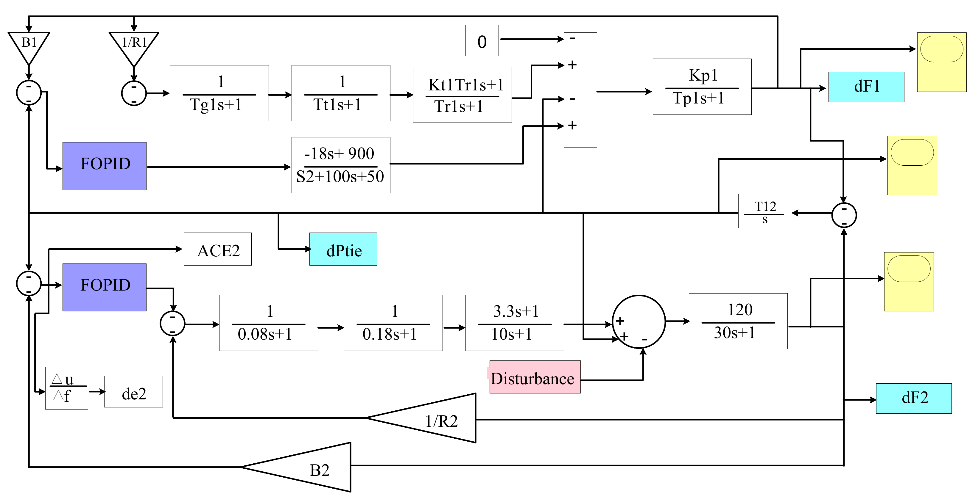
2. System Modeling

The proposed system involves various renewable energy sources (RESs) such as PV arrays and wind power plants. Furthermore, the proposed system contains thermal power plants. The model of the system under study can be mathematically represented by the models of a wind turbine, PV array, and thermal power plant.

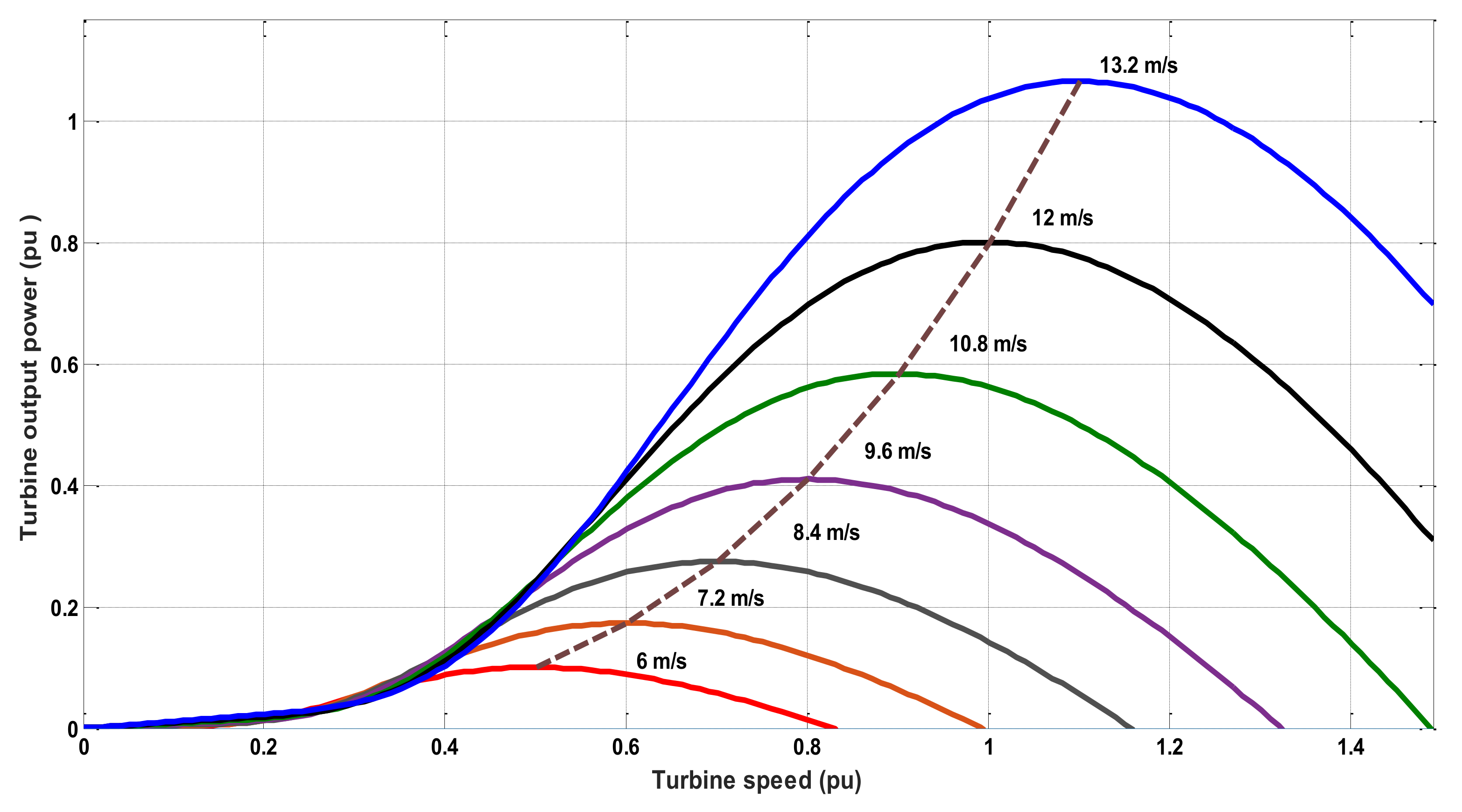
2.1. Model of Wind Turbine Plant

The wind turbine (WT) extracted power is proportional to the cube of wind speed and the power coefficient ($C_p$), which relies on tip-speed ratio defined by ($\lambda$) and blade-pitch angle defined by ($\beta$). The optimal value of the power coefficient reflects in the extraction of maximum power from the wind turbine. The ratio of tip speed can be given as [47,48]

$$\lambda =\left({\omega }_{t}R\right)/V_w$$

(1)

where R represents the radius of WT, $V_w$ denotes the speed of wind, and ${\omega }_t$ represents the rotor speed. The WT mechanical power can be formulated as

$$P_W=\frac{1}{2}\rho A{C}_p\left(\lambda ,\beta \right)V_w^3$$

(2)

where $\rho$ is the air density and A represents the WT area. Equation (3) represents the formula of the power coefficient.

$$C_p=\left(0.44-0.0167\times \beta \right)sin\left(\frac{\pi (\lambda -2)}{15-0.3\beta }\right)-0.00184\left(\lambda -3\right)\beta .$$

(3)

Figure 1 depicts the relation between the WT mechanical power and its rotational speed at variable wind speeds. Each curve in the figure has a maximum power point to be tracked, and this point changes based on the wind speed.

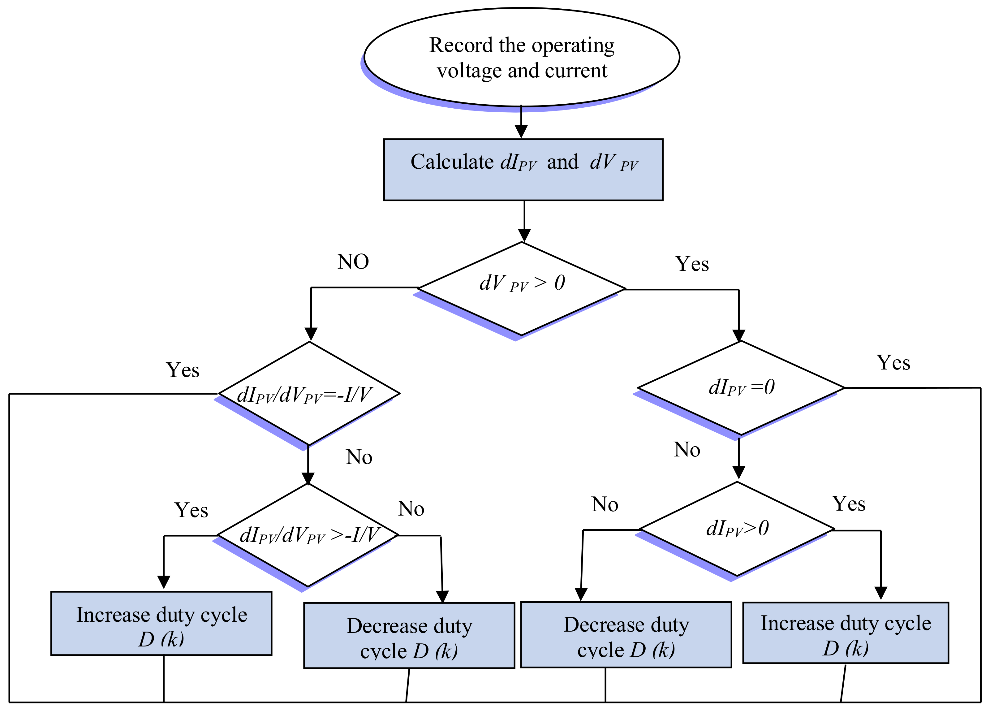
2.2. PV Array Model

PV arrays consist of several PV modules that are interlinked in series to raise the voltage and in parallel to raise the current of the PV array and to meet the load demand. These objectives depend mainly on both the solar irradiance and the surface temperature. The PV array voltage is determined by [49]

$$V=\left(\frac{N_sϵZ{T}_a}{Q}\right)ln\left[\frac{N_{p}G{I}_{ph}-I+N_p{I}_o}{N_p{I}_o}\right]-\left(\frac{N_{s}I{R}_s}{N_p}\right)$$

(4)

where V and I represent the PV array voltage and current, respectively, Q denotes electron charge, Z represent the Boltzmann coefficient, $T_a$ represents surface temperature, $ϵ$ denotes completion factor, $N_s$ and $N_p$ are the total count of series and parallel connected cells, $R_s$ represents the series resistance, $I_{ph}$ represents the photocurrent of the PV module, $I_o$ is the leakage current, and G represents irradiance. The maximum power point of the PV module can be tracked by trackers [50]. To achieve this object, several algorithms have been used for tracking the maximum power. Among them, the incremental conductance (INC) methodology is commonly used. This method is employed to manage the boost converter’s duty cycle of the PV system. Figure 2 illustrates a flowchart of this method. The proposed method relies on the following equation [51]:

$$\begin{array}{c}\hfill \left\{\begin{array}{c}\frac{d{P}_{PV}}{d{v}_{PV}}>0\mathrm{At}\mathrm{right}\mathrm{side}\mathrm{of}\mathrm{MPP},\hfill \\ \frac{d{P}_{PV}}{d{v}_{PV}}=0\mathrm{At}\mathrm{MPP},\hfill \\ \frac{d{P}_{PV}}{d{v}_{PV}}<0\mathrm{At}\mathrm{left}\mathrm{side}\mathrm{of}\mathrm{MPP}\hfill \end{array}\right.\end{array}$$

(5)

The PV system transfer functions can be expressed as [52]

$$G_1=\left(\frac{s^2}{s^2+{\omega }^2}\right)\left(\frac{V\left(s^2+{\omega }^2\right)\left(s^2+2{\omega }^2\right)}{k{s}^2\left(s^2+4{\omega }^2\right)}\right)\left(\frac{1-e^{-s{T}_s}}{s{T}_s}\right)$$

(6)

$$G_2=\left(\frac{\frac{M_1}{LC}}{s^2+\frac{1}{RC}s+\frac{1}{LC}}\right)\left(\frac{1-e^{\frac{-s{T}_s}{2}}}{1+e^{\frac{-s{T}_s}{2}}}\right)\left(\frac{M_2}{1+s{T}_s}\right)$$

(7)

where $\omega$ denotes angular frequency of the electric grid, R, L, and C represent the output parameters of the converter, $M_1$ equals the voltage gain of the chopper circuit, $M_2$ equals the inverter voltage gain, and $T_s$ represents the sampling period.

2.3. Thermal Power Plant Model

A thermal power plant comprises synchronous generators units, a steam turbine, a speed-governor system, and a reheating system. The transfer functions of these individual units are mathematically modeled as [53]

-

Governor model

$$G_g=\frac{K_g}{T_{g}s+1}$$

(8)

-

Reheater model

$$G_r=\frac{K_r{T}_{r}s+1}{T_{r}s+1}$$

(9)

-

Turbine model

$$G_t=\frac{K_t}{T_{t}s+1}$$

(10)

-

Generator model

$$G_{g}en=\frac{K_p}{T_{p}s+1}$$

(11)

where $K_g$, $K_t$, $K_r$, and $K_p$ represent gains of the governor, turbine, reheater, and generator, $T_g$, $T_t$, $T_r$, and $T_p$ represent the time constant of governor, turbine, reheater, and generator. All components are simulated as first-order transfer functions.

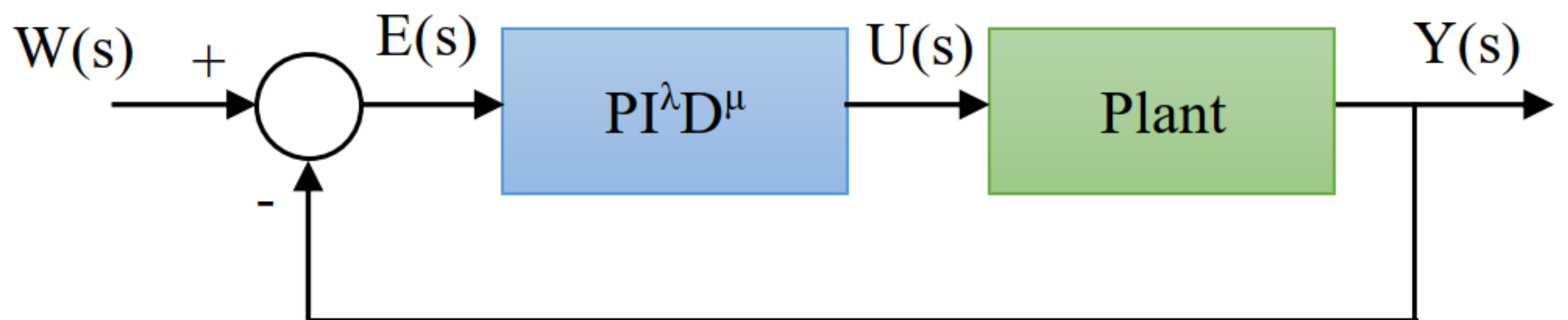
3. Problem Formulation

The fractional-order proportional–integral–derivative (FOPID) controller was proposed by Podlubny [50]. It has a higher performance than the traditional PID for many closed-loop control systems. It has five parameters, $K_p$, $K_i$, and $K_d$, that represent gains of the proportional, integral, and derivative parts, the integrator order defined by ($\lambda$), and the derivative order defined by ($\mu$). A simple schematic diagram of the proposed controller is illustrated in Figure 3. Its transfer function is formulated as

$$G_{c}s=K_p+\frac{K_i}{s^{\lambda }}+K_d{s}^{\mu }\lambda ,\mu >0$$

(12)

These five parameters of the FOPID controller are fully designed using a novel modified HGS algorithm. The integral time absolute error (ITAE) comprising the frequency and tie-line power changes is selected as the fitness function. The design process is demonstrated in Figure 4. This fitness function is expressed as

$$ITAE=\underset{0}{\overset{t}{\int }}t.\left[\sum _{j=1}^{M_{unit}}|\Delta F_j+\Delta P_{tie,j}\right]dt,$$

(13)

where t denotes the simulation time, $M_{unit}$ is the number of interconnected areas, and $\Delta F_j$ and $\Delta P_{tie,j}$ are the frequency change in the $j^{th}$ area and the tie-line power number j.

The constraints of the optimization problem are as follows:

$$\begin{array}{cc}\hfill & K_{Pj}^{Low}\le K_{Pj}\le K_{Pj}^{High}\hfill \\ \hfill & K_{Ij}^{Low}\le K_{Ij}\le K_{Ij}^{High}\hfill \\ \hfill & K_{dj}^{Low}\le K_{dj}\le K_{dj}^{High}\forall \in N_c\hfill \\ \hfill & {\lambda }_j^{Low}\le {\lambda }_j\le {\lambda }_j^{High}\hfill \\ \hfill & {\mu }_j^{Low}\le {\mu }_j\le {\mu }_j^{High}\hfill \end{array}$$

(14)

where $Low$ and $High$ represent the lower and higher limits of parameters, and $N_C$ represents FOPID controller numbers. The parameters’ lower and higher limits are between [0, 1].

In this article, two systems are studied: the 1st consists of a two-area system that includes PV and thermal power plants. The LFC diagram of the system is illustrated in Figure 5. The 2nd system contains PV, WT, and 2 thermal power plants and is clearly indicated in Figure 6.

4. The Proposed Solution Methodology

4.1. Overview Hunger Games Search Optimizer

Yang et al. [54] have developed a new optimizer named the hunger games search (HGS) optimizer to imitate animals’ starvation-driven activities and behavior. The animals have two social strategies while searching for food: in the first strategy, the animals behave as a team. In contrast, a few animals are separated and dependant on their abilities to catch the food (self-dependent manner) in the second strategy. To implement these social manners, Yang et al. [54] formulated the mathematical equations of HGS as

$$\begin{array}{c}\hfill \overrightarrow{Y_i(t+1)}=\left\{\begin{array}{c}Gam{e}_1:\overrightarrow{Y_i\left(t\right)}.\left(1+randn\left(1\right)\right)R_1<f,........\left(i\right)\hfill \\ Gam{e}_2:\overrightarrow{{\omega }_{1_i}}\left(t\right).\overrightarrow{Y_i^b\left(t\right)}+\overrightarrow{D_i}\left(t\right).\overrightarrow{{\omega }_{2_i}}\left(t\right).|\overrightarrow{Y_i^b\left(t\right)}-\overrightarrow{Y_i\left(t\right)}|r_1>L,R_2>B\left(t\right),........\left(ii\right)\hfill \\ Gam{e}_3:\overrightarrow{{\omega }_{1_i}}\left(t\right).\overrightarrow{Y_i^b\left(t\right)}-\overrightarrow{D_i}\left(t\right).\overrightarrow{{\omega }_{2_i}}\left(t\right).|\overrightarrow{Y_i^b\left(t\right)}-\overrightarrow{Y_i\left(t\right)}|r_1>L,R_2<B\left(t\right)........\left(iii\right)\hfill \end{array}\right.\end{array}$$

(15)

where $\overrightarrow{Y_i^b\left(t\right)}$ is the location of the best solution at the current iteration (t), the $\overrightarrow{Y_i\left(t\right)}$ is the position of the $i^{th}$ animal. The $\overrightarrow{{\omega }_1}$ and $\overrightarrow{{\omega }_2}$ are the weights of hunger to perform the hunger-driven signals. The $\overrightarrow{{\omega }_1}$ refers to the error in getting the right position whereas the $\overrightarrow{{\omega }_2}$ is considered to handle the effectiveness of starvation on the range of activity. The multiplication of $\overrightarrow{Y_i\left(t\right)}and\left(1+randn\left(1\right)\right)$ of Equation (15) indicates the random manner of the hungry animal while looking for its foods at the current position. The $|\overrightarrow{Y_i^b\left(t\right)}-\overrightarrow{Y_i\left(t\right)}|$ of Equation (15) refers to the range of activity of the $i^{th}$ animal in t. To adjust the range of activity, the weight ($\overrightarrow{{\omega }_2}$) is multiplied in that part ($|\overrightarrow{Y_i^b\left(t\right)}-\overrightarrow{Y_i\left(t\right)}|$). Hence, the animal can stop searching when it is complete. Adding and subtracting the part of $\overrightarrow{{\omega }_1}.\overrightarrow{Y_i^b\left(t\right)}$ in the second and third lines of Equation (15) implements the current animal becoming acquainted with its peers when nearing the food location and then continuing looking for food again at the current location. The f is a constant number chosen to be 0.03 by relying on the original article on HGS [54]. The $\overrightarrow{D}$ is a ranging controller; it has values in the interval of [−b, b]. The $\overrightarrow{D}$ is employed to manage the range of the activity. Therefore, it is slowly decreased to 0. Both $R_1$ and $R_2$ are random values in the range of [0, 1]. $randn\left(1\right)$ is a random number drawn from a normal distribution. The decision making of Equation (15) is controlled by the variable B that can be calculated through Equation (16) [54].

$$B_i\left(t\right)=sech\left(|Fu{n}_i\left(t\right)-G^{*}\left(t\right)|\right)i\in 1,2,3,....,N$$

(16)

where the $Fu{h}_i$ is the objective function value of the $i^{th}$ animal at t, $G^{*}$ is the best objective function obtained so far at t. The variable N is the total number of animals, and $sech\left(x\right)$ illustrates the hyperbolic function that equals $1/Cosh\left(x\right)$.

Once again, by observing the main equations of HGS in Equation (15), the first line of it is an implementation of the self-dependent manner. In comparison, the second and third lines are emulations of the team cooperation work. The motion of the animals based on the second and third lines is mainly restricted by three variables: $\overrightarrow{D}$, $\overrightarrow{{\omega }_1}$, and  $\overrightarrow{{\omega }_2}$. Yang et al. [54] adjusted these variables by performing the following equations.

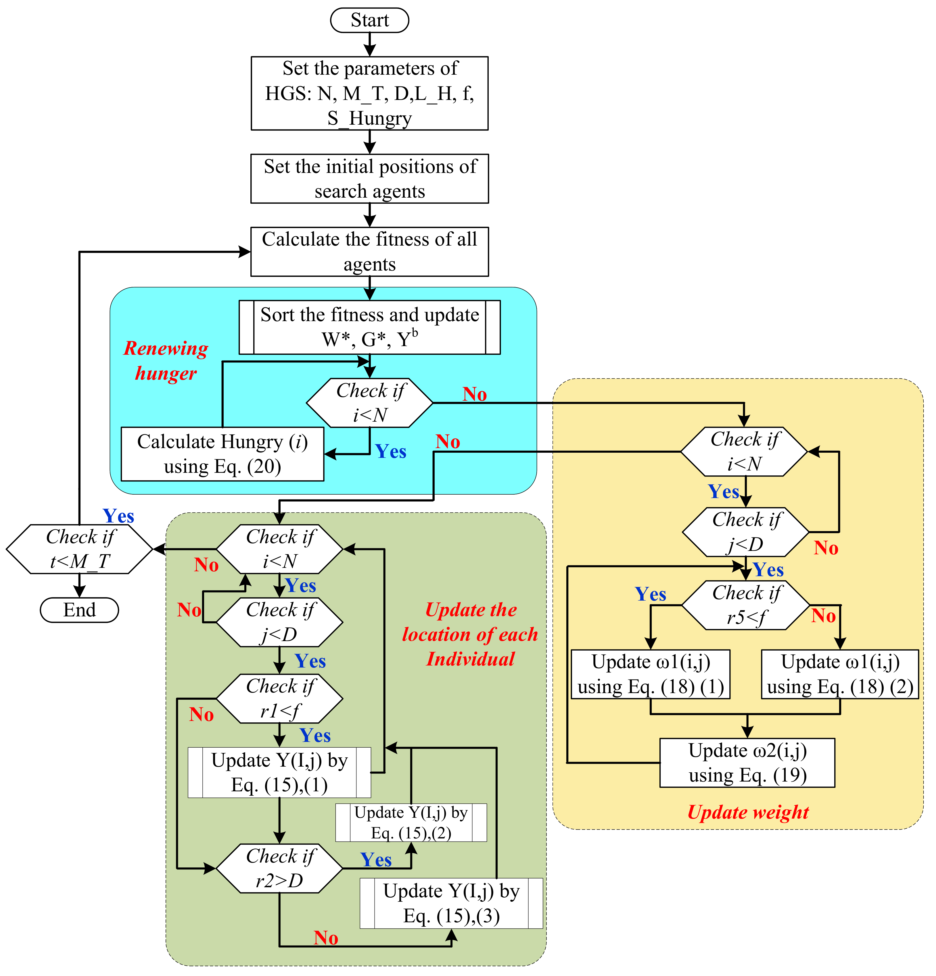
• Tuning the ranging controller ($\overrightarrow{D}$): Yang et al. [54] suggested the following equation to implement the animal shrinking manner across the iterations (t):

  $$\begin{array}{c}\overrightarrow{D_i\left(t\right)}=2\times shrin{k}_i\left(t\right)\times R_3-shrin{k}_i\left(t\right),\hfill \\ where,\hfill \\ shrin{k}_i\left(t\right)=2\times \left(1-\frac{t}{M_T}\right)\hfill \end{array}$$

  (17)

  where $M_T$ illustrates the total number of iterations, $R_3$ refers to a random number in the interval of [0,1].
• Tuning the weights ($\overrightarrow{{\omega }_1}$) and ($\overrightarrow{{\omega }_2}$): Yang et al. [54] used the following equations to boost the animals’ manner when looking for their food.

  $$\overrightarrow{{\omega }_{1_i}}\left(t\right)=\left\{\begin{array}{c}Hungr{y}_i\left(t\right).\frac{M}{S\_Hungry\left(t\right)}\times R_4{R}_5<f,\hfill \\ 1R_5>f\hfill \end{array}\right.$$

  (18)

  $$\overrightarrow{{\omega }_{2_i}}\left(t\right)=\left(1-exp\left(-|Hungr{y}_i\left(t\right)-S\_Hungry\left(t\right)|\right)\right)\times R_6\times 2$$

  (19)

  where the random values in Equations (18) and (19) are symbolized by $R_4$, $R_5$, and $R_6$. The $Hungr{y}_i\left(t\right)$ is the $i^{th}$ hungry animal while $S\_Hungry\left(t\right)$ is the sum of the hungry feelings of all animals at $\left(t\right)$. The formula of $Hungr{y}_i\left(t\right)$ is modeled as follows:

  $$Hungr{y}_i\left(t\right)=\left\{\begin{array}{c}0Fu{n}_i\left(t\right)==G^{*}\left(t\right)\hfill \\ Hungr{y}_i\left(t\right)+N\_Hungr{y}_i\left(t\right)Fu{n}_i\left(t\right)=G^{*}\left(t\right)\hfill \end{array}\right.$$

  (20)

  where $N\_Hungr{y}_i\left(t\right)$ is a new hungry animal which is considered if the objective function of the $i^{th}$ animal is not equal to the best-attained objective so far $G^{*}$. The respective new hunger of various animals is different. Therefore, in [54], the new hunger $N\_Hungry$ formula is considered as

  $$\begin{array}{c}N\_Hungr{y}_i\left(t\right)=\left\{\begin{array}{cc}C\_H\times (1+R)\hfill & \hfill K\_H<C\_H\\ K\_H_i\left(t\right)\hfill & \hfill K\_H\ge C\_H.\end{array}\right.,\hfill \\ where\hfill \\ K\_H_i\left(t\right)=\frac{Fu{n}_i\left(t\right)-G^{*}\left(t\right)}{W^{*}\left(t\right)-G^{*}\left(t\right)}\times R_7\times 2\times (High-Low)\hfill \end{array}$$

  (21)

  where $W^{*}\left(t\right)$ is the worst value of fitness achieved so far. $High$ and $Low$ are the the search space upper and lower limits, respectively. The $C\_H$ is a constant value recommended to be 100 [54]. The HGS flowchart is shown in Figure 7.

4.2. The Proposed Modified Hunger Games Search Optimizer

Discovering efficient solutions and avoiding the local solutions in the first iterations are principle targets achieved via enhancing the diversification stage of the optimizer. Therefore, in this work, the non-uniform mutation operator is employed to enhance the diversity of the solutions and discover the search landscape efficiently, as mentioned in Algorithm 1. The structure of the proposed MHGS is reported in Algorithm 2, where it starts with a set of initial solutions then assesses the objective function using this initialization. For the maximum number of iterations $M_T$, the initial solutions are updated and the non-uniform mutation operator is performed to ensure the diversity of the solutions. The weights ${\omega }_{1,2}$ and the algorithm parameters are modified throughout the iterations. The previously mentioned processes are repeated until the termination phenomenon is satisfied.

Algorithm 1 The non-uniform mutation operator.

1: for Each agent i ($i=g_1+1,...,n$) do 2:    for Each dimension j ($j=1,...,d$) do 3:      if rand < 0.1 then 4:         $a=rand(1,D)$; $N_{d\times d}$ = $diag\left(a\right)$; 5:         if round (rand) = 0 then 6:           Update the agent position according       $U_{ij}=U_{ij}+N_{d\times d}\left(Max\_B_j-U_{ij}\right){\left(1-\frac{t}{Ma{x}_T}\right)}^2$ 7:         else if round (rand) = 1 then 8:           Update the particle position according       $U_{ij}=U_{ij}+N_{d\times d}\left(U_{ij}-Min\_B_j\right){\left(1-\frac{t}{Ma{x}_T}\right)}^2$ 9:         end if 10:      end if 11:    end for 12: end for

Algorithm 2:Steps of MHGS.

1: Set the MHGS parameters; N agents, number of iterations ($M_T$), $L,D,L_H,S\_hunger$, 2: Calculate the initial solutions matrix. 3: Set t = 1. 4: while termination criteria are not met do 5:    Evaluate the objective function (Fun) for all search agents. 6:    Update the Best ($G^{*}$), Worst ($W^{*}$) values of the fitness function and assign the best solutions ($Y^b$). 7:    Calculate the Hungry using Equation (20). 8:    Update the weight ${\omega }_1$ using Equation (18). 9:    Update the weight ${\omega }_2$ using Equation (19). 10:    for The first group of the agents ($i=1,...,N$) do 11:      Update the agents’ locations using Equation (15)(i)... 12:      Update the agents’ locations using Equation (15)(ii, iii). 13:      Apply Algorithm 1 to implement non-uniform mutation operator for the solutions. 14:    end for 15:    t = t + 1. 16: end while 17: Display the best solutions.

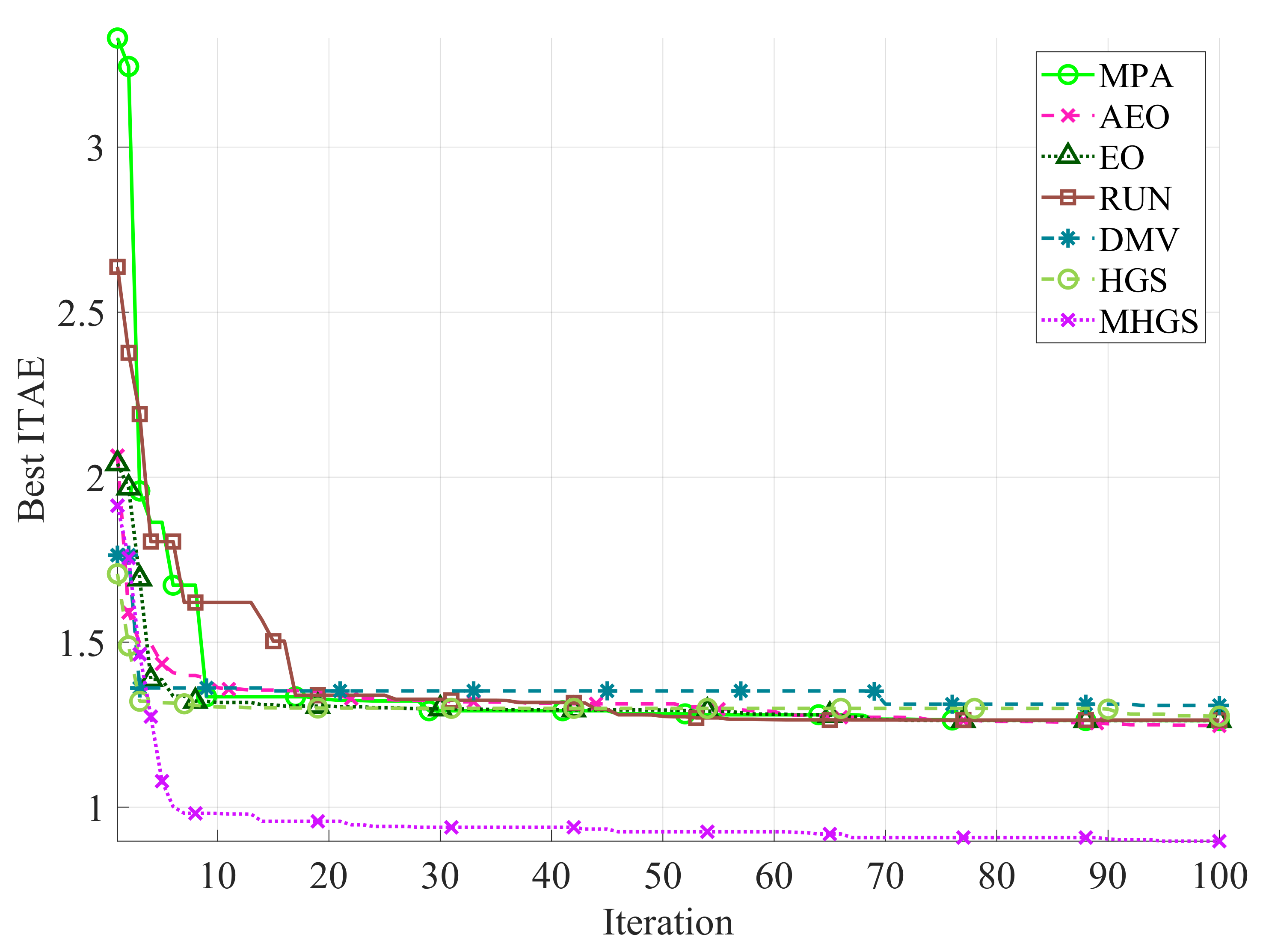
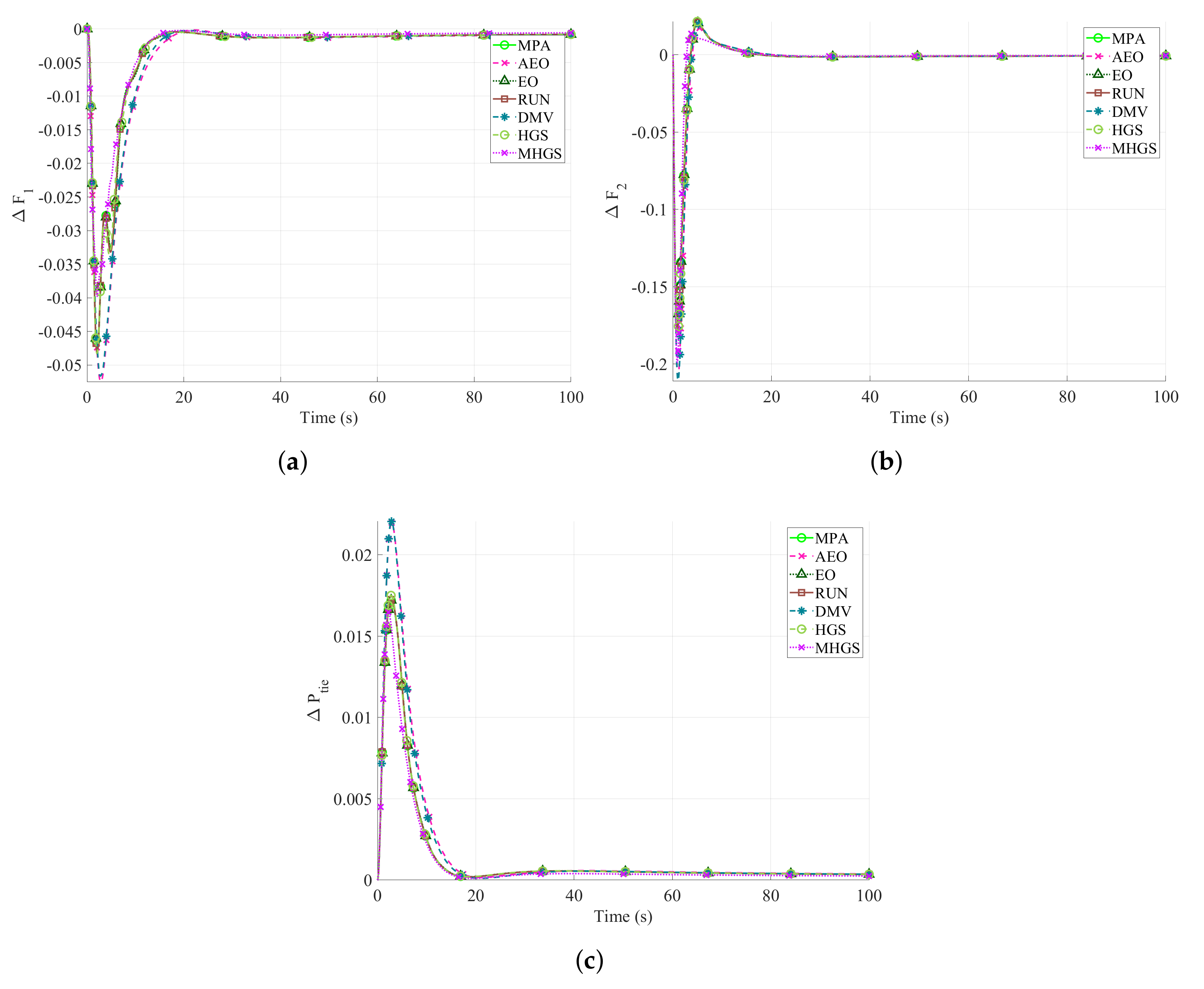
5. Simulation and Discussion

The analysis is performed using two interconnected systems.

The proposed MHGS is applied to identify the FOPID controllers that are involved in the systems to maintain zero deviations in the frequencies and tie-line powers. The MHGS is compared to a set of recent optimization algorithms that have been implemented with the same settings, including the marine predators algorithm (MPA) [55], artificial ecosystem based optimization (AEO) [56], equilibrium optimizer (EO) [57], Runge-Kutta based optimizer (RUN) [58], movable damped wave algorithm (DMV) [59], and the classical version of HGS [54]. The analysis is implemented on the MATLAB 2018 platform. For a fair assessment, a population size of 30 and 100 iterations are considered for all approaches.

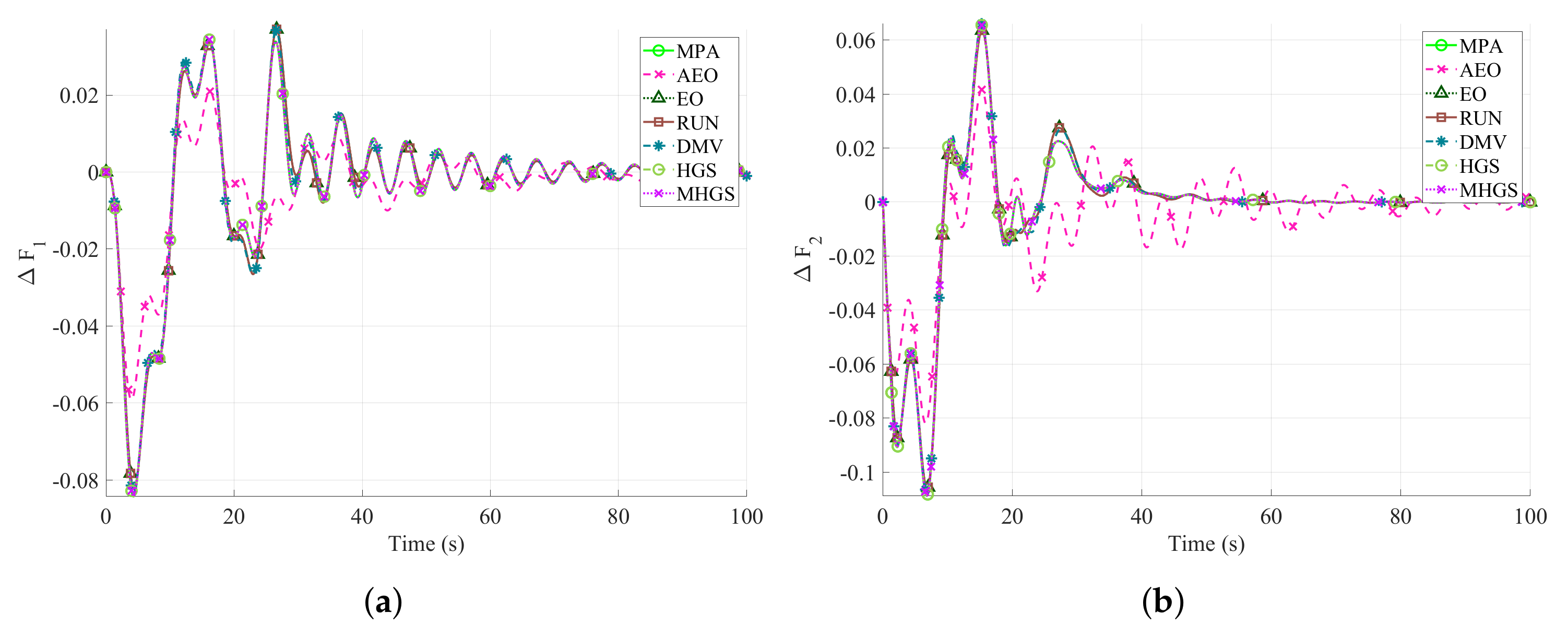
5.1. PV Interconnected System

In this section, two interconnected units including a grid-connected PV unit with MPPT and reheat thermal power generation unit are considered while assessing the proposed optimizer. The studied MATLAB/Simulink scheme is displayed in Figure 8, and the data of this system are from [60].

The analysis in this part is performed for two cases: the first one involves adding step disturbance in the PV plant of +10%. For the second case, a sudden step change in the disturbance in the PV unit is included where three levels of disruption are recognized: first, 50%, then suddenly increasing to 80%, and reducing to 20%. The considered levels of the disturbances for the two cases are depicted in Figure 9.

Table 1. The FOPID controller’s identified parameters by the tested techniques in the case of two interconnected units.

Para	Algorithms
	MPA	AEO	EO	RUN	DMV	HGS	MHGS
$K_{P1}$	$0.0100$	$0.0111$	$0.0108$	$0.0105$	$0.8209$	$0.0351$	$0.8318$
$K_{I1}$	$0.1850$	$0.1004$	$0.1885$	$0.1884$	$0.9423$	$0.1868$	$0.2046$
${\lambda }_1$	$1.0000$	$0.9961$	$1.0000$	$1.0000$	$1.0000$	$1.0000$	$0.0255$
$K_{d1}$	$0.0100$	$0.5348$	$0.0114$	$0.0116$	$1.0000$	$0.0100$	$0.4157$
${\mu }_1$	$0.8423$	$0.9952$	$0.9110$	$0.7097$	$0.3430$	$1.0000$	$0.3270$
$K_{P2}$	$1.0000$	$0.9996$	$1.0000$	$1.0000$	$1.0000$	$1.0000$	$0.9846$
$K_{I2}$	$1.0000$	$0.6182$	$1.0000$	$1.0000$	$0.6394$	$1.0000$	$0.9531$
${\lambda }_2$	$0.8125$	$0.8607$	$0.8115$	$0.8126$	$0.8618$	$0.8111$	$0.8592$
$K_{d2}$	$1.0000$	$0.5541$	$0.9974$	$0.9804$	$0.5061$	$0.9113$	$0.9994$
${\mu }_2$	$0.5000$	$0.5032$	$0.5000$	$0.5000$	$0.5000$	$0.5000$	$0.0057$
ITAE	$g1.2622$	$1.2465e+00$	$1.2623e+00$	$1.2639e+00$	$1.3083e+00$	$1.2761e+00$	$8.9726e-01$
ITSE	$5.5548e-02$	$8.2327e-02$	$5.5578e-02$	$5.5943e-02$	$8.2496e-02$	$5.7300e-02$	$5.1801e-02$
IAE	$3.9261e-01$	$5.2427e-01$	$3.9402e-01$	$3.9239e-01$	$5.0609e-01$	$3.9448e-01$	$3.4179e-01$

reports the attained optimal gains of FOPID controller based LFC by the proposed optimizer and its counterparts in the case of adding 10% disturbance to the PV unit. Moreover, the corresponding ITAE, ITSE, and IAE are listed to assess the proposed MHGS’s performance. The illustrated data show the ability of the proposed MHGS in providing the most efficient values for the FOPID controllers’ parameters that achieve the least ITAE, ITSE, and IAE of 0.89726, $5.1801\times {10}^{-2}$, and $0.34179$, respectively. In contrast, the MPA, which is considered the best comparable counterpart, achieves ITAE, ITSE, and IAE of 1.2622, $5.5548\times {10}^{-2}$, and $0.39261$, respectively. The ITAE, ITSE, and IAE are related to tie-line power and frequency deviations. Their lowest values are the metrics for the best performance and the highest efficient control. Accordingly, the MHGS confirms its reliability in this stage.

The decaying of the fitness function throughout the iterations is the other sector that should be evaluated. Thus, the convergence properties of the MPA, AEO, EO, RUN, DMV, HGS, and the proposed MHGS are depicted in Figure 10. The curves illustrate the excellence of the proposed MHGS in decaying rapidly to high-quality solutions that attain the lowest ITAE at a smaller number of iterations. Due to this, the authors can affirm that the non-linear mutation enhanced the optimizer in discovering the search space efficiently compared with the classical HGS and the others.

Response properties of frequencies and tie-line powers’ fluctuations at 10 in PV plant.

Studying the PV and thermal interconnected system response using the optimal FOPID controller parameters obtained via the implemented techniques is the core of this work to demonstrate the proposed optimizer’s robustness. Therefore, the time responses of the frequencies and tie-line powers’ deviations are exhibited in Figure 11. The plotted curves affirm that the FOPID controller based MHGS attains the best steady state response with acceptable specifications compared with the others. Moreover, the MHGS based system reaches a steady deviation nearly at zero, as displayed in Figure 11. In contrast, the AEO and DMV based systems show high values in the overshoot and take a long time to reach stability. Using the curves of Figure 11, several metrics are computed in

Table 2. Response properties of frequencies and tie-line powers’ fluctuations at 10% load disturbance in PV plant.

Specifications
Algs	RiseTime	SettlingTime	SettlingMin	SettlingMax	Overshoot	Undershoot	Peak	PeakTime
	${\mathit{t}}_{\mathit{r}}$$\left(\mathit{s}\right)$	${\mathit{t}}_{\mathit{s}}$$\left(\mathit{s}\right)$	${\mathit{A}\mathit{m}\mathit{b}}_{\mathit{s}\mathit{M}\mathit{i}\mathit{n}}$$\left(\mathit{H}\mathit{z}\right)$	${\mathit{A}\mathit{m}\mathit{b}}_{\mathit{s}\mathit{M}\mathit{a}\mathit{x}}$$\left(\mathit{H}\mathit{z}\right)$	${\mathit{O}}_{\mathit{s}}$	${\mathit{U}}_{\mathit{s}}$	$\mathit{P}\mathit{e}\mathit{a}\mathit{k}$$\left(\mathit{H}\mathit{z}\right)$	${\mathit{t}}_{\mathit{P}\mathit{e}\mathit{a}\mathit{k}}$$\left(\mathit{s}\right)$
$\Delta$$F_1$
MPA AEO EO RUN DMV HGS MHGS	$1.7576e-01$ $1.1729e-01$ $1.7576e-01$ $1.7590e-01$ $1.1621e-01$ $1.7521e-01$ $1.2157e-01$	$1.2482e+01$ $1.5710e+01$ $1.2470e+01$ $1.2550e+01$ $1.4878e+01$ $1.2835e+01$ $1.2379e+01$	$-4.8137e-02$ $-5.2508e-02$ $-4.7971e-02$ $-4.8337e-02$ $-5.1644e-02$ $-4.8277e-02$ $-3.9804e-02$	$-4.1416e-04$ $-1.5583e-04$ $-4.3716e-04$ $-4.2506e-04$ $-2.3702e-04$ $-4.7306e-04$ $-2.2556e-04$	$-4.1416e-04$ $-1.5583e-04$ $-4.3716e-04$ $-4.2506e-04$ $-2.3702e-04$ $-4.7306e-04$ $-2.2556e-04$	$-4.8137e-02$ $-5.2508e-02$ $-4.7971e-02$ $-4.8337e-02$ $-5.1644e-02$ $-4.8277e-02$ $-3.9804e-02$	$4.8137e-02$ $5.2508e-02$ $4.7971e-02$ $4.8337e-02$ $5.1644e-02$ $4.8277e-02$ $3.9804e-02$	$2.0614e+00$ $2.8230e+00$ $2.0614e+00$ $2.0517e+00$ $2.7289e+00$ $2.0245e+00$ $2.0477e+00$
$\Delta$$F_2$
MPA AEO EO RUN DMV HGS MHGS	$2.8367e-03$ $2.7923e-03$ $2.8588e-03$ $2.8344e-03$ $2.6787e-03$ $2.8710e-03$ $1.9977e-03$	$1.3607e+01$ $1.4357e+01$ $1.3600e+01$ $1.3561e+01$ $1.4425e+01$ $1.3378e+01$ $1.2254e+01$	$-1.7809e-01$ $-2.0812e-01$ $-1.7819e-01$ $-1.7901e-01$ $-2.1090e-01$ $-1.8229e-01$ $-1.9902e-01$	$2.0675e-02$ $1.7210e-02$ $2.0565e-02$ $2.0917e-02$ $1.9630e-02$ $2.1413e-02$ $1.3549e-02$	$2.0675e-02$ $1.7210e-02$ $2.0565e-02$ $2.0917e-02$ $1.9630e-02$ $2.1413e-02$ $1.3549e-02$	$-1.7809e-01$ $-2.0812e-01$ $-1.7819e-01$ $-1.7901e-01$ $-2.1090e-01$ $-1.8229e-01$ $-1.9902e-01$	$1.7809e-01$ $2.0812e-01$ $1.7819e-01$ $1.7901e-01$ $2.1090e-01$ $1.8229e-01$ $1.9902e-01$	$8.7053e-01$ $1.0006e+00$ $8.7054e-01$ $8.7056e-01$ $1.0068e+00$ $8.8298e-01$ $8.4905e-01$
$\Delta$P${}_{tie}$
MPA AEO EO RUN DMV HGS MHGS	$1.2019e-01$ $1.0793e-01$ $1.2091e-01$ $1.2015e-01$ $1.0475e-01$ $1.2141e-01$ $9.7142e-02$	$1.3126e+01$ $1.5311e+01$ $1.3175e+01$ $1.3092e+01$ $1.4869e+01$ $1.3057e+01$ $1.3057e+01$	$1.8732e-04$ $1.4996e-04$ $1.9921e-04$ $1.8482e-04$ $1.0061e-04$ $2.0125e-04$ $9.8693e-05$	$1.7192e-02$ $2.1967e-02$ $1.7207e-02$ $1.7252e-02$ $2.2052e-02$ $1.7502e-02$ $1.6472e-02$	$1.7192e-02$ $2.1967e-02$ $1.7207e-02$ $1.7252e-02$ $2.2052e-02$ $1.7502e-02$ $1.6472e-02$	$1.8732e-04$ $1.4996e-04$ $1.9921e-04$ $1.8482e-04$ $1.0061e-04$ $2.0125e-04$ $9.8693e-05$	$1.7192e-02$ $2.1967e-02$ $1.7207e-02$ $1.7252e-02$ $2.2052e-02$ $1.7502e-02$ $1.6472e-02$	$2.7655e+00$ $2.8677e+00$ $2.7623e+00$ $2.7623e+00$ $2.8285e+00$ $2.7348e+00$ $2.1932e+00$

such as the settling time $\left(t_s\right)$ $\left(s\right)$, rise time $\left(t_r\right)$ $\left(s\right)$, the minimum and maximum setting values ($Am{b}_{sMin}$, $Am{b}_{sMax}$), overshoot ($O_s$), undershoot($U_s$), and the peak level $\left(Hz\right)$ as well as its time ($t_{Peak}$) $\left(s\right)$. The response properties of the frequencies and power deviations of Table 2 show that the MHGS based system reaches stability the fastest. as it has the shortest settling time and it is the most well constructed as it has the lowest peak, overshoots at early times, and then becomes steady, as indicated in Figure 11.

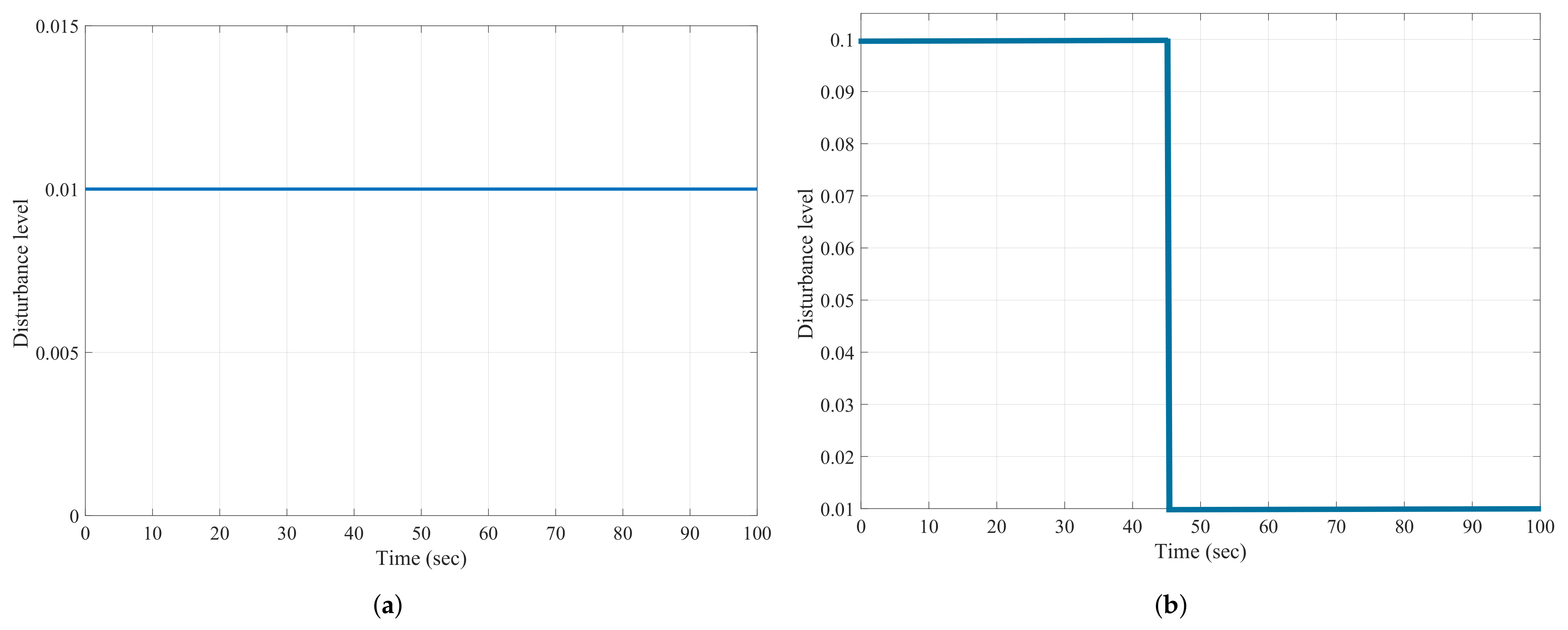
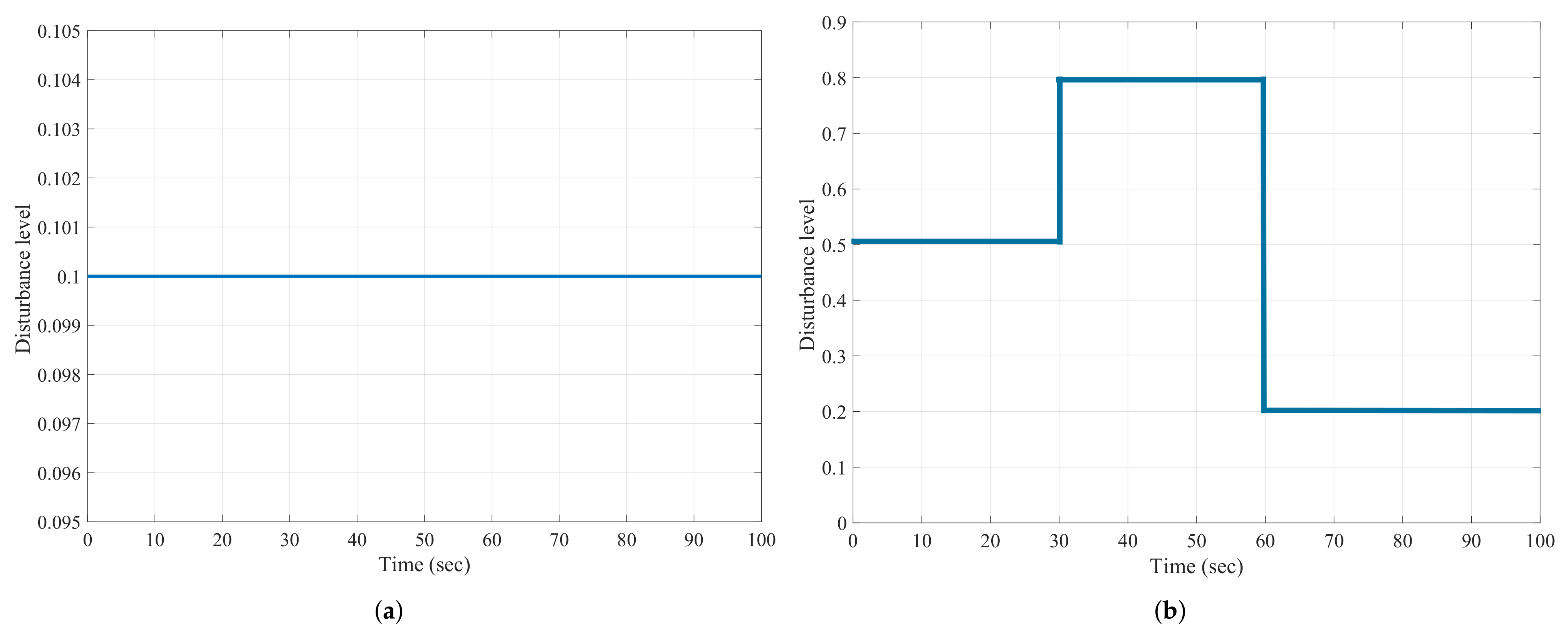
Robustness Evaluation under Variable Disturbance: Two Areas

The investigation on the reliability and robustness of the proposed MHGS based system did not stop at studying the system response while using 10% disturbance on the PV unit, as we used three levels of disturbances that changed suddenly, as shown in Figure 9b, to evaluate the MHGS based controllers’ performance. The time responses of the deviations in frequencies and tie-line powers throughout the simulation time are depicted in Figure 12. By inspecting the curves, one can detect that the MHGS based system responds rapidly with minimum peaks and becomes steady. However, the peaks and settling time achieved via the controllers based on the others are remarkable, especially while using AEO and DMV based controllers. Accordingly, the proposed MHGS confirms and provides evidence on its superiority and outstanding performance compared to the others. Thus, it is an efficient approach in identifying the FOPID controller parameters for two interconnected areas using various disturbances.

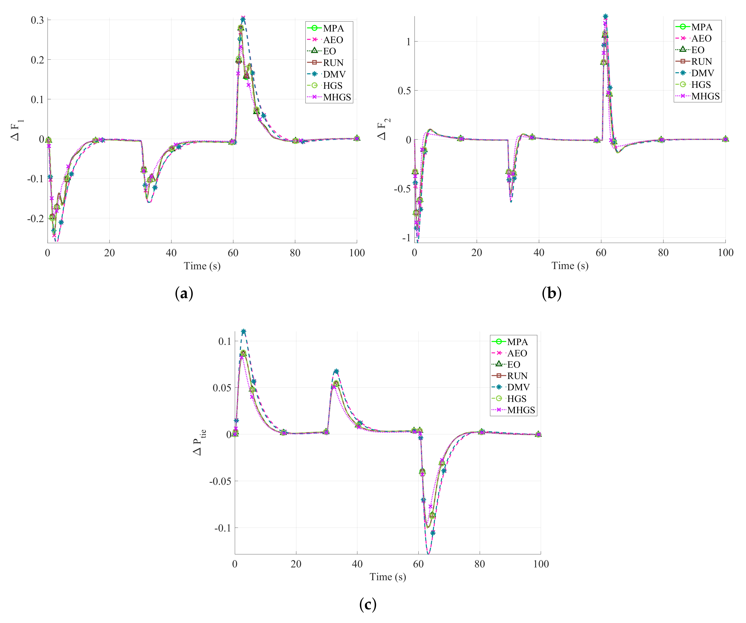
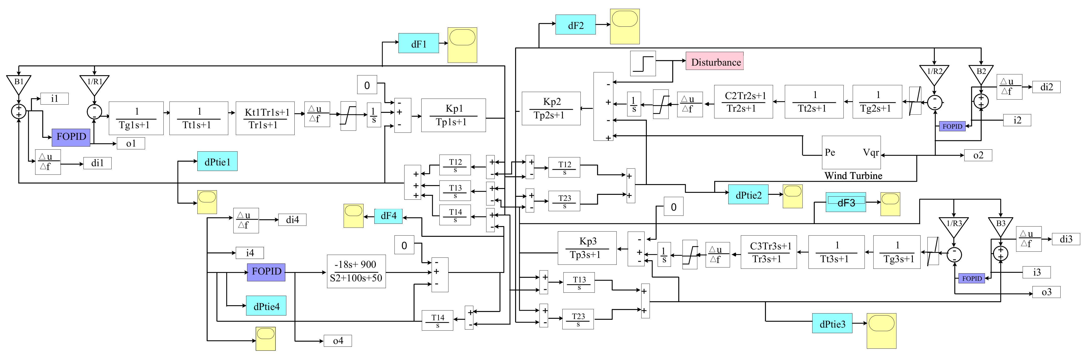
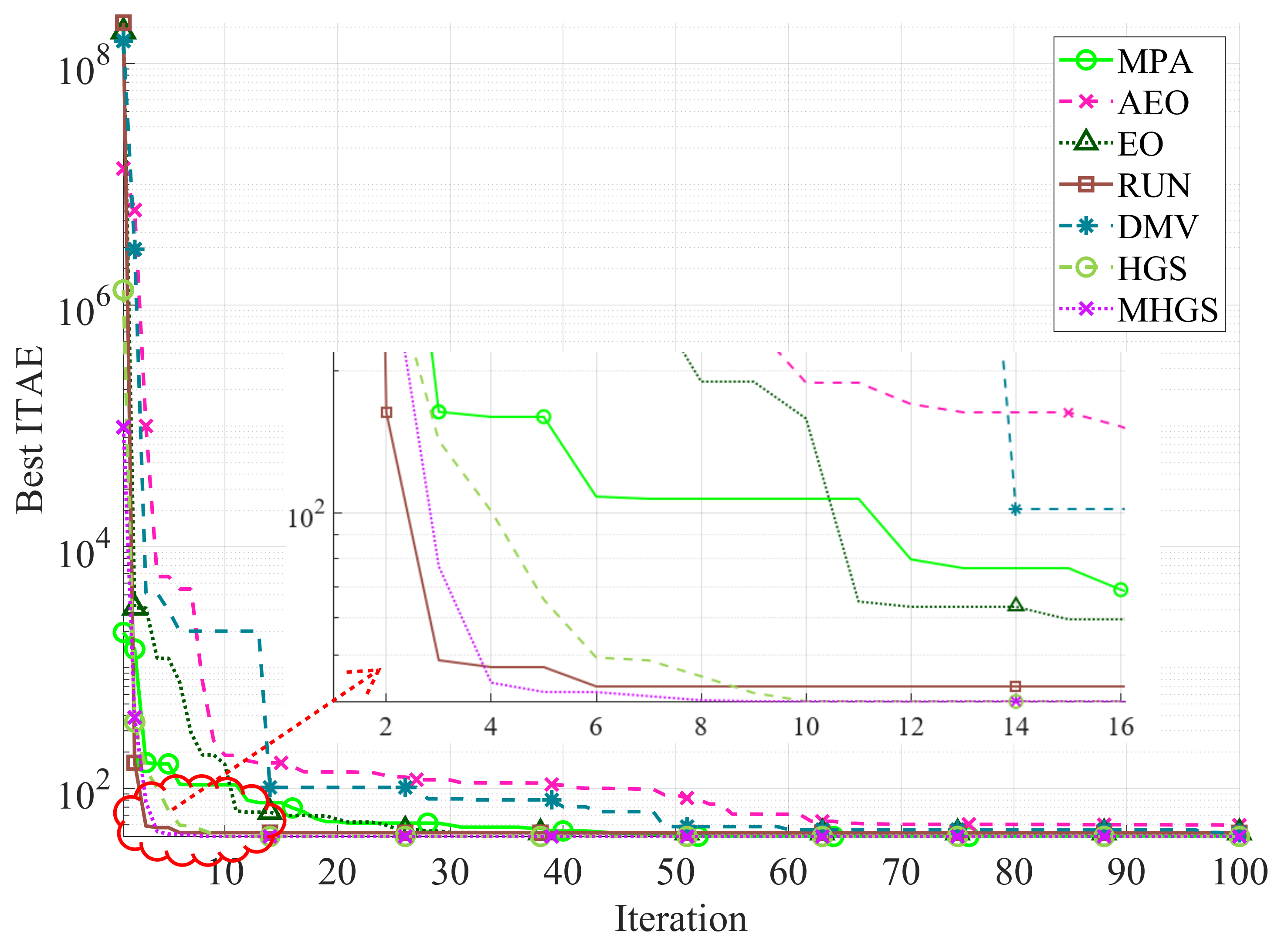
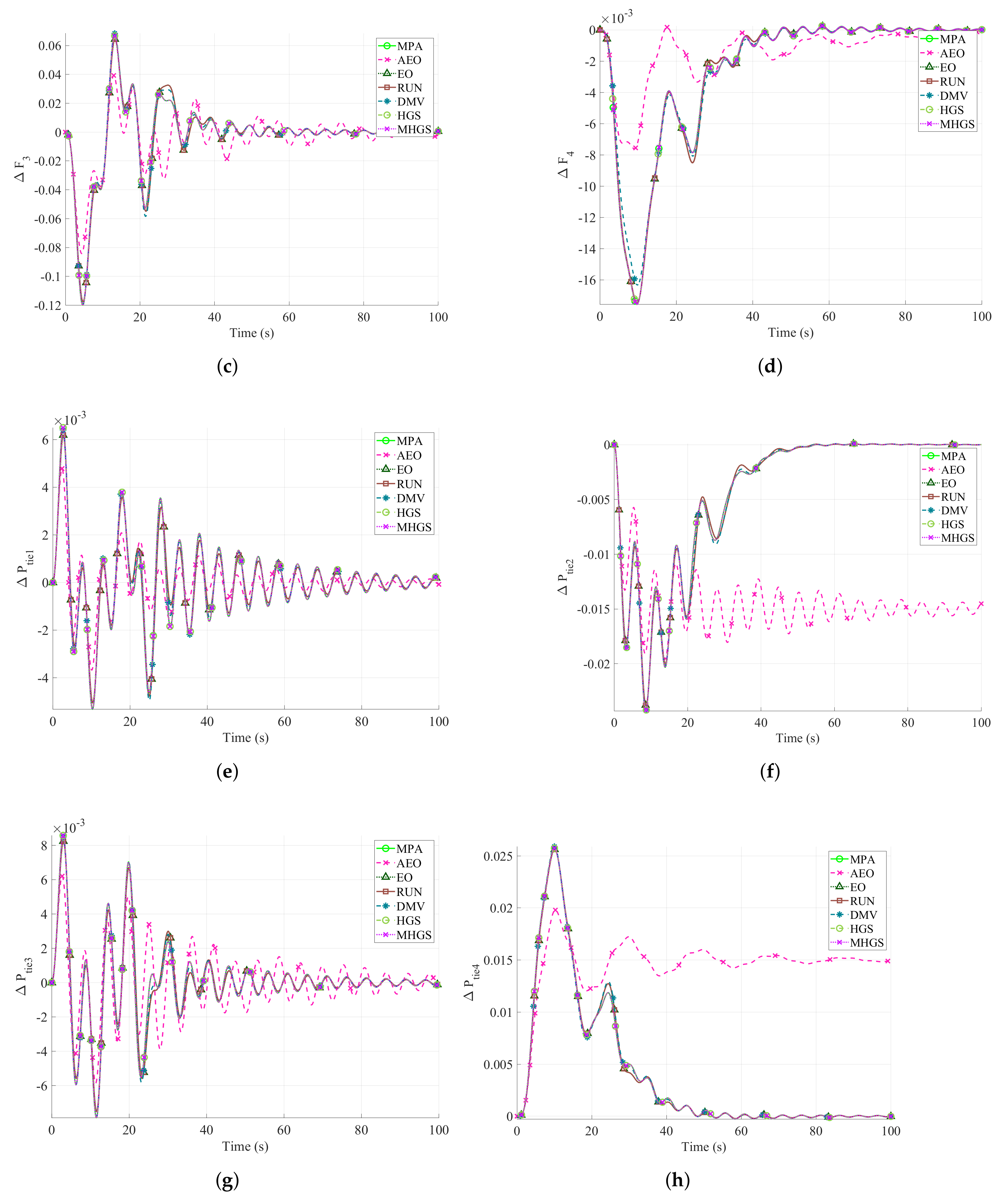
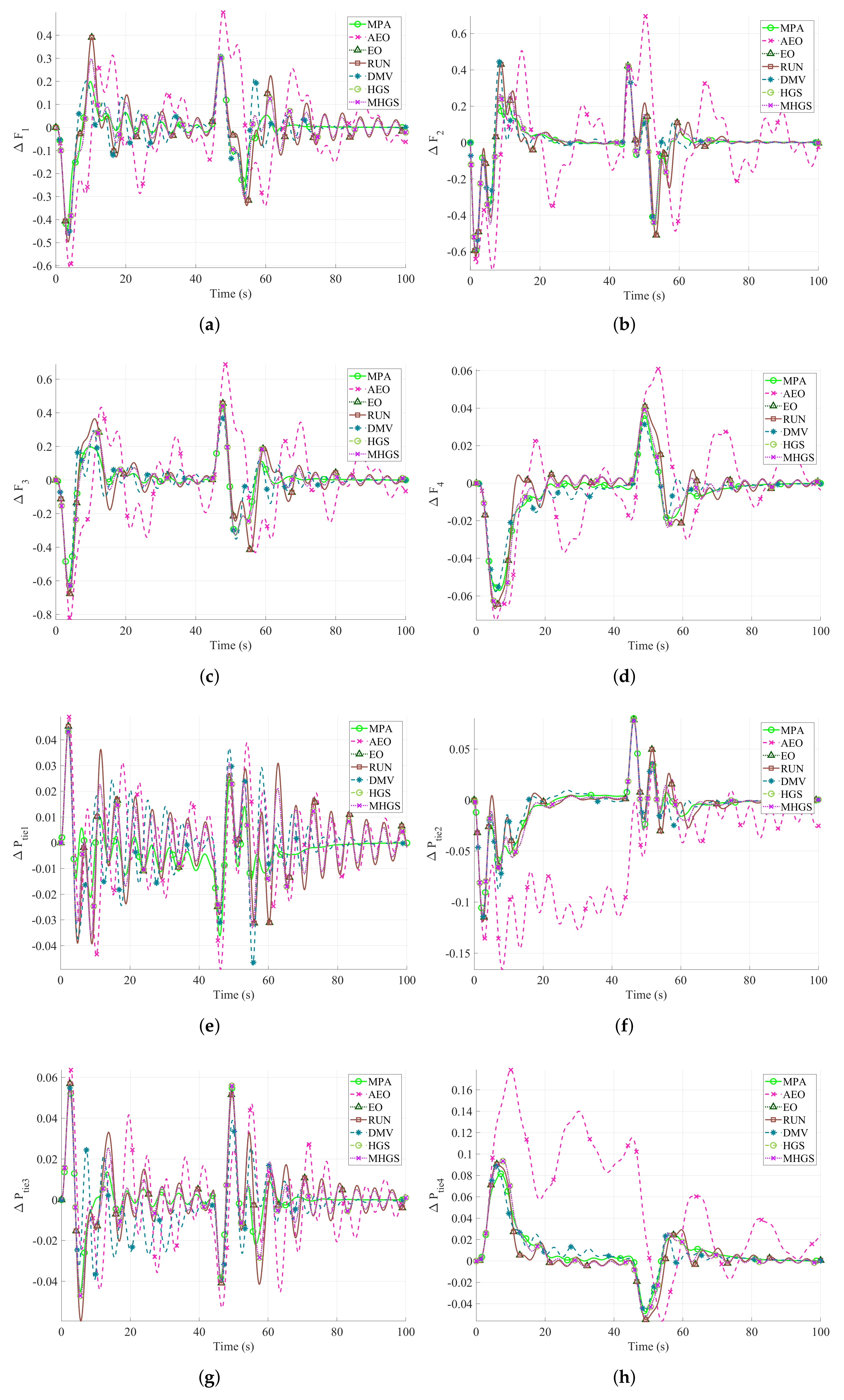
5.2. Four Interconnected Systems

In this section, the developed controller is examined with 4 different plants of PV, wind turbine (WT), and 2 thermal units. The non-linear based model of thermal plants is considered via generation rate constraints (GRCs) and governor dead-band (GDB). The constructed system using Simulink is presented in Figure 13. The data of this system are available in [61,62].

The simulations in this part are implemented by considering two different load disturbances. The first one is +1% occurring in the load of area 2 (WT based plant). The second one is a sudden step change in the disturbance of the WT based plant where two levels of disruption are recognized: 10% and then a sudden reduction to 1%. The considered levels of the disturbances for the two cases are drawn in Figure 14. The variation in the fitness function (ITAE) with iteration number for the proposed MHGS in comparison with the others for a 1% disturbance applied on a WT based plant (area 2) is shown in Figure 15. The curves confirm the superiority of the proposed MHGS as it achieves the minimum fitness function.

The time responses of frequency perturbations, $\Delta$$F_1$, $\Delta$$F_2$, $\Delta$$F_3$, and $\Delta$$F_4$, and tie-line powers, $\Delta$$P_{tie2}$, $\Delta$$P_{tie2}$, $\Delta$$P_{tie3}$, and $\Delta$$P_{tie4}$, achieved via the proposed approach and the others for such disturbance are presented in Figure 16. From the presented curves of Figure 16, it can be clearly observed that tie-line power and frequency deviations completely vanished with the FOPID controllers optimized via the proposed MHGS. On the other hand, there are some approaches that failed in keeping these violations to zero, such as AEO. For $\Delta$$P_{tie2}$ and $\Delta$$P_{tie4}$, the FOPID optimized via the AEO keeps the deviations at −0.015 and 0.015 pu, respectively. The optimal parameters of the FOPID controller obtained via the proposed approach and the others in the case of load disturbance of 1% on a WT based plant, in addition to the fitness function (ITAE), ITSE, and IAE, are tabulated in

Table 3. The FOPID controller’s identified parameters by the tested techniques in the case of four interconnected units.

Para	Algorithms
	MPA	AEO	EO	RUN	DMV	HGS	MHGS
$K_{P1}$	$1.0000$	$0.0806$	$0.8794$	$0.4533$	$0.2240$	$1.0000$	$0.0100$
$K_{I1}$	$1.0000$	$0.1471$	$0.0100$	$0.0107$	$0.0105$	$0.0100$	$0.1454$
${\lambda }_1$	$1.0000$	$0.2866$	$0.0100$	$0.0105$	$0.0681$	$0.0100$	$0.9082$
$K_{d1}$	$1.0000$	$0.8554$	$0.1157$	$0.0103$	$0.0257$	$0.0100$	$0.0271$
${\mu }_1$	$0.6489$	$0.2407$	$0.7277$	$0.5477$	$0.0917$	$0.0147$	$0.0115$
$K_{P2}$	$1.0000$	$0.0101$	$1.0000$	$1.0000$	$0.7759$	$1.0000$	$1.0000$
$K_{I2}$	$1.0000$	$0.0125$	$1.0000$	$1.0000$	$1.0000$	$1.0000$	$1.0000$
${\lambda }_2$	$1.0000$	$0.1930$	$1.0000$	$1.0000$	$1.0000$	$1.0000$	$1.0000$
$K_{d2}$	$1.0000$	$0.0687$	$0.0100$	$0.0100$	$0.8075$	$1.0000$	$1.0000$
${\mu }_2$	$0.0100$	$0.9665$	$0.0100$	$0.0101$	$0.0863$	$0.0100$	$0.0100$
$K_{P3}$	$1.0000$	$0.1424$	$0.0100$	$0.0100$	$0.0881$	$0.0100$	$0.1453$
$K_{I3}$	$0.0100$	$0.1957$	$0.0105$	$0.0102$	$1.0000$	$0.0100$	$0.0100$
${\lambda }_3$	$1.0000$	$0.0383$	$0.0121$	$0.0101$	$1.0000$	$0.0623$	$0.0152$
$K_{d3}$	$1.0000$	$0.4543$	$0.0102$	$0.0101$	$0.0384$	$0.2925$	$0.2917$
${\mu }_3$	$1.0000$	$0.0743$	$0.0524$	$0.9373$	$0.7900$	$1.0000$	$1.0000$
$K_{P4}$	$0.0100$	$0.0104$	$0.0100$	$0.0100$	$0.0100$	$0.0100$	$0.0100$
$K_{I4}$	$0.0100$	$0.0189$	$0.0100$	$0.0100$	$0.0113$	$0.0100$	$0.0100$
${\lambda }_4$	$0.0100$	$0.1411$	$0.0100$	$0.0100$	$0.0100$	$0.0100$	$0.0100$
$K_{d4}$	$0.0100$	$0.0102$	$0.0100$	$0.0100$	$0.0310$	$0.0100$	$0.0100$
${\mu }_4$	$1.0000$	$0.0854$	$1.0000$	$1.0000$	$1.0000$	$1.0000$	$1.0000$
ITAE	$4.0027e+01$	$4.9618e+01$	$4.2947e+01$	$4.2948e+01$	$4.2861e+01$	$4.0027e+01$	$4.0026e+01$
ITSE	$4.5713e-01$	$2.2382e-01$	$4.6841e-01$	$4.6840e-01$	$4.6517e-01$	$4.5713e-01$	$4.5713e-01$
IAE	$1.0172e+00$	$1.4192e+00$	$1.0172e+00$	$1.0172e+00$	$9.8577e-01$	$1.0172e+00$	$1.0171e+00$

. Regarding to the obtained results, the developed method outperformed the others in terms of ITAE, achieving the best value of $4.0026$, while AEO achieved the worst value of $4.9618e+00$. Moreover, regarding to the results of ITSE and IAE, the proposed MHGS achieved good values of $4.57137e-01$ and $1.0171e-01$, respectively.

It is standard practice to investigate the time responses of the frequencies and tie-line powers’ violations when installing FOPID controllers optimized via new approach, and this is done by calculating the performance metrics, such as rise time ($t_r$), settling time $t_s$, settling minimum ($Am{b}_{sMin}$), settling maximum ($Am{b}_{sMax}$), overshoot ($O_s$), undershoot ($U_s$), peak value ($Peak$), and peak time ($t_{Peak}$), which are calculated and exhibited in

Table 4. Response properties of frequencies and tie-line powers’ deviations at 1% load disturbance applied on area 2 of the four connected systems.

Specifications
Algs	RiseTime	Settling Time	Settling Min	Settling Max	Overshoot	Undershoot	Peak	PeakTime
	${\mathit{t}}_{\mathit{r}}$$\left(\mathit{s}\right)$	${\mathit{t}}_{\mathit{s}}$$\left(\mathit{s}\right)$	${\mathit{A}\mathit{m}\mathit{b}}_{\mathit{s}\mathit{M}\mathit{i}\mathit{n}}$$\left(\mathit{H}\mathit{z}\right)$	${\mathit{A}\mathit{m}\mathit{b}}_{\mathit{s}\mathit{M}\mathit{a}\mathit{x}}$$\left(\mathit{H}\mathit{z}\right)$	${\mathit{O}}_{\mathit{s}}$	${\mathit{U}}_{\mathit{s}}$	$\mathit{P}\mathit{e}\mathit{a}\mathit{k}$$\left(\mathit{H}\mathit{z}\right)$	${\mathit{t}}_{\mathit{P}\mathit{e}\mathit{a}\mathit{k}}$$\left(\mathit{s}\right)$
$\Delta$$f_1$
MPA AEO EO RUN DMV HGS MHGS	$3.1988e-01$ $2.9175e-01$ $2.9208e-01$ $2.9210e-01$ $3.1936e-01$ $3.1989e-01$ $3.1989e-01$	$9.8531e+01$ $9.6929e+01$ $9.8261e+01$ $9.8261e+01$ $9.8538e+01$ $9.8531e+01$ $9.8231e+01$	$-8.4281e-02$ $-5.9199e-02$ $-8.2374e-02$ $-8.2374e-02$ $-8.3448e-02$ $-8.4281e-02$ $-8.4281e-02$	$3.4395e-02$ $2.0937e-02$ $3.7086e-02$ $3.7087e-02$ $3.6873e-02$ $3.4395e-02$ $3.4395e-02$	$2.7469e-02$ $1.3705e-02$ $2.7448e-02$ $2.7442e-02$ $2.9078e-02$ $2.7469e-02$ $2.7469e-02$	$-8.4281e-02$ $-5.9199e-02$ $-8.2374e-02$ $-8.2374e-02$ $-8.3448e-02$ $-8.4281e-02$ $-8.4281e-02$	$8.4281e-02$ $5.9199e-02$ $8.2374e-02$ $8.2374e-02$ $8.3448e-02$ $8.4281e-02$ $8.4281e-02$	$4.2754e+00$ $3.9601e+00$ $4.3539e+00$ $4.3532e+00$ $4.2860e+00$ $4.2733e+00$ $4.2756e+00$
$\Delta$$f_2$
MPA AEO EO RUN DMV HGS MHGS	$5.1341e-04$ $1.5191e-02$ $5.2317e-04$ $5.2329e-04$ $5.6583e-04$ $5.1341e-04$ $5.1340e-04$	$4.8225e+01$ $9.9174e+01$ $4.8615e+01$ $4.8615e+01$ $4.8442e+01$ $4.8225e+01$ $4.8224e+01$	$-1.0878e-01$ $-3.3055e-02$ $-1.0627e-01$ $-1.0627e-01$ $-1.0734e-01$ $-1.0878e-01$ $-1.0878e-01$	$6.5512e-02$ $4.1619e-02$ $6.3582e-02$ $6.3582e-02$ $6.6057e-02$ $6.5512e-02$ $6.5512e-02$	$5.3133e-02$ $7.4760e-03$ $2.6207e-02$ $2.6212e-02$ $2.5240e-02$ $5.3157e-02$ $5.3141e-02$	$-1.0878e-01$ $-6.4994e-02$ $-1.0481e-01$ $-1.0478e-01$ $-1.0148e-01$ $-1.0878e-01$ $-1.0878e-01$	$1.0878e-01$ $8.1953e-02$ $1.0627e-01$ $1.0627e-01$ $1.0734e-01$ $1.0878e-01$ $1.0878e-01$	$6.7717e+00$ $6.5943e+00$ $6.8138e+00$ $6.8133e+00$ $6.7756e+00$ $6.7727e+00$ $6.7721e+00$
$\Delta$$f_3$
MPA AEO EO RUN DMV HGS MHGS	$1.1905e-02$ $3.9484e-01$ $9.7584e-03$ $9.7602e-03$ $1.2295e-02$ $1.1905e-02$ $1.1905e-02$	$7.2618e+01$ $9.7610e+01$ $6.2780e+01$ $6.2780e+01$ $7.2617e+01$ $7.2618e+01$ $7.2617e+01$	$-5.2768e-02$ $-8.4206e-02$ $-5.4889e-02$ $-5.4892e-02$ $-5.8411e-02$ $-5.2768e-02$ $-5.2768e-02$	$6.6739e-02$ $3.9258e-02$ $6.4380e-02$ $6.4382e-02$ $6.8406e-02$ $6.6739e-02$ $6.6738e-02$	$6.6739e-02$ $3.9258e-02$ $6.4380e-02$ $6.4382e-02$ $6.8406e-02$ $6.6739e-02$ $6.6738e-02$	$-1.2004e-01$ $-2.9537e-02$ $-1.1756e-01$ $-1.1756e-01$ $-1.1928e-01$ $-1.2004e-01$ $-1.2004e-01$	$1.2004e-01$ $8.4206e-02$ $1.1756e-01$ $1.1756e-01$ $1.1928e-01$ $1.2004e-01$ $1.2004e-01$	$4.6501e+00$ $4.3625e+00$ $4.7170e+00$ $4.7171e+00$ $4.6654e+00$ $4.6493e+00$ $4.6487e+00$
$\Delta$$f_4$
MPA AEO EO RUN DMV HGS MHGS	$4.7598e-02$ $5.5075e-01$ $4.9277e-02$ $5.0518e-02$ $1.3983e-02$ $3.2849e-02$ $4.8022e-02$	$5.1013e+01$ $9.0159e+01$ $4.6587e+01$ $4.6597e+01$ $4.6563e+01$ $5.1009e+01$ $5.1013e+01$	$-3.8968e-04$ $-7.6004e-03$ $-2.7190e-04$ $-2.7192e-04$ $-2.9518e-04$ $-3.8970e-04$ $-3.8966e-04$	$2.6047e-04$ $1.7406e-04$ $2.2740e-04$ $2.2733e-04$ $2.1890e-04$ $2.6047e-04$ $2.6047e-04$	$2.6047e-04$ $1.7406e-04$ $2.2740e-04$ $2.2733e-04$ $2.1890e-04$ $2.6047e-04$ $2.6047e-04$	$-1.7563e-02$ $-7.6004e-03$ $-1.7478e-02$ $-1.7478e-02$ $-1.6331e-02$ $-1.7563e-02$ $-1.7563e-02$	$1.7563e-02$ $7.6004e-03$ $1.7478e-02$ $1.7478e-02$ $1.6331e-02$ $1.7563e-02$ $1.7563e-02$	$9.6425e+00$ $8.9862e+00$ $9.6902e+00$ $9.7036e+00$ $9.7956e+00$ $9.6789e+00$ $9.6783e+00$
$\Delta$P${}_{tie1}$
MPA AEO EO RUN DMV HGS MHGS	$1.2327e-01$ $1.6931e-02$ $1.3202e-01$ $1.3204e-01$ $1.2268e-01$ $1.2327e-01$ $1.2327e-01$	$9.9373e+01$ $9.9081e+01$ $9.7746e+01$ $9.7746e+01$ $9.9385e+01$ $9.9373e+01$ $9.9372e+01$	$-5.3218e-03$ $-3.6759e-03$ $-5.0574e-03$ $-5.0574e-03$ $-5.3180e-03$ $-5.3218e-03$ $-5.3217e-03$	$6.4990e-03$ $2.0852e-03$ $6.1900e-03$ $6.1900e-03$ $6.4049e-03$ $6.4990e-03$ $6.4990e-03$	$1.9320e-03$ $2.8133e-03$ $1.8202e-03$ $1.8193e-03$ $1.2851e-03$ $1.9317e-03$ $1.9317e-03$	$-1.0640e-03$ $-1.4903e-03$ $-1.3319e-03$ $-1.3353e-03$ $-5.5398e-04$ $-1.0621e-03$ $-1.0600e-03$	$6.4990e-03$ $4.7852e-03$ $6.1900e-03$ $6.1900e-03$ $6.4049e-03$ $6.4990e-03$ $6.4990e-03$	$2.6434e+00$ $2.3702e+00$ $2.6837e+00$ $2.6839e+00$ $2.6506e+00$ $2.6402e+00$ $2.6396e+00$
$\Delta$P${}_{tie2}$
MPA AEO EO RUN DMV HGS MHGS	$1.3715e-01$ $2.0287e+00$ $4.1995e-02$ $4.1990e-02$ $7.5824e-02$ $1.3715e-01$ $1.3716e-01$	$4.8447e+01$ $9.9306e+01$ $4.8413e+01$ $4.8413e+01$ $4.8342e+01$ $4.8447e+01$ $4.8347e+01$	$-1.0693e-04$ $-1.9589e-02$ $-8.0386e-05$ $-8.0374e-05$ $-8.0983e-05$ $-1.0693e-04$ $-1.0693e-04$	$9.5781e-05$ $-5.7313e-03$ $8.6965e-05$ $8.6978e-05$ $1.0881e-04$ $9.5781e-05$ $9.5780e-05$	$9.5781e-05$ $-1.1420e-02$ $8.6965e-05$ $8.6978e-05$ $1.0881e-04$ $9.5781e-05$ $9.5780e-05$	$-1.8690e-02$ $-1.9073e-02$ $-1.8126e-02$ $-1.8126e-02$ $-1.8546e-02$ $-1.8690e-02$ $-1.8690e-02$	$2.4327e-02$ $1.9589e-02$ $2.3838e-02$ $2.3838e-02$ $2.4285e-02$ $2.4327e-02$ $2.4327e-02$	$8.5767e+00$ $1.3838e+01$ $8.6487e+00$ $8.6482e+00$ $8.5949e+00$ $8.5769e+00$ $8.5797e+00$
$\Delta$P${}_{tie3}$
MPA AEO EO RUN DMV HGS MHGS	$7.6821e-03$ $5.5891e-02$ $9.0602e-03$ $9.0602e-03$ $7.7799e-03$ $7.6823e-03$ $7.6823e-03$	$9.7251e+01$ $9.9600e+01$ $9.7358e+01$ $9.7358e+01$ $9.7264e+01$ $9.7251e+01$ $9.7251e+01$	$-7.8777e-03$ $-5.8583e-03$ $-7.5137e-03$ $-7.5137e-03$ $-7.8173e-03$ $-7.8777e-03$ $-7.8777e-03$	$7.0310e-03$ $4.9957e-03$ $6.7016e-03$ $6.7017e-03$ $7.0634e-03$ $7.0310e-03$ $7.0309e-03$	$2.0739e-03$ $3.0002e-03$ $8.7849e-04$ $8.7811e-04$ $1.4150e-03$ $2.0725e-03$ $2.0740e-03$	$-1.6633e-03$ $-3.5553e-03$ $-3.0034e-04$ $-2.9069e-04$ $-1.0067e-03$ $-1.6639e-03$ $-1.6750e-03$	$8.5740e-03$ $6.2064e-03$ $8.2416e-03$ $8.2416e-03$ $8.4841e-03$ $8.5740e-03$ $8.5740e-03$	$2.9478e+00$ $2.6778e+00$ $2.9952e+00$ $2.9947e+00$ $2.9606e+00$ $2.9494e+00$ $2.9487e+00$
$\Delta$P${}_{tie4}$
MPA AEO EO RUN DMV HGS MHGS	$4.4028e+00$ $3.9547e+00$ $4.2065e+00$ $4.2071e+00$ $9.4141e-02$ $4.4028e+00$ $4.4028e+00$	$5.1028e+01$ $7.8125e+01$ $4.6877e+01$ $4.6877e+01$ $4.6770e+01$ $5.1028e+01$ $5.1027e+01$	$-2.6127e-04$ $1.2032e-02$ $-2.2564e-04$ $-2.2567e-04$ $-2.7623e-04$ $-2.6127e-04$ $-2.6127e-04$	$3.2721e-04$ $1.9796e-02$ $2.9376e-04$ $2.9376e-04$ $4.7387e-04$ $3.2721e-04$ $3.2721e-04$	$2.5737e-02$ $1.9796e-02$ $2.5615e-02$ $2.5615e-02$ $2.5899e-02$ $2.5737e-02$ $2.5737e-02$	$-2.6127e-04$ $1.2032e-02$ $-2.2564e-04$ $-2.2567e-04$ $-2.7623e-04$ $-2.6127e-04$ $-2.6127e-04$	$2.5737e-02$ $1.9796e-02$ $2.5615e-02$ $2.5615e-02$ $2.5899e-02$ $2.5737e-02$ $2.5737e-02$	$9.9860e+00$ $1.0244e+01$ $1.0040e+01$ $1.0040e+01$ $9.9766e+00$ $9.9853e+00$ $9.9847e+00$

. The obtained responses via the proposed MHGS are correlated to MPA, AEO, EO, RUN, DMV, and HGS. The results show the dominance of the proposed MHGS compared to the others for all responses of frequencies and tie-line powers’ variations.

Robustness Evaluation under Variable Disturbance: Four Areas

In this part, the reliability of the proposed optimizer is investigated under dynamic changes in the disturbance. Therefore, the recognized second load disturbance applied on a WT based plant (area 2) in four interconnected systems is not a fixed level like the first one. Two levels of disruption are applied. The first one is 10% which is continued for 45 s and then reduces suddenly to 1% for the remaining time interval of the simulation, up to 100 s. The application of this dynamic disturbance is important in order to monitor the performance of the proposed FOPID controllers. The optimal parameters of FOPID controllers obtained via the proposed MHGS given in Table 3 are used in the dynamic load disturbance, and the time responses of frequencies and tie-line powers’ deviations are traced and plotted in Figure 17.

The FOPID-LFC controllers work in two time intervals. The first one runs from 0 s to 45 s, in which the load disturbance of 10% is considered. The second one runs from 45 s to 100 s, in which the disturbance is 1%. The designed controllers via the proposed approach succeeded in removing the deviations of all frequencies and tie-line powers in the two considered intervals. On the other hand, the controllers designed via AEO failed in achieving the target for $\Delta$$F_2$, $\Delta$$P_{tie2}$, and $\Delta$$P_{tie4}$. Moreover, the AEO based controllers generate large oscillations.

It is clear that the proposed method incorporating MHGS succeeded in designing reliable and efficient FOPID-LFC controllers that are capable of removing the disruptions of frequencies and tie-line powers for a multi-interconnected system subjected to either static or dynamic load disturbances.

6. Conclusions and Perspectives

A modified hunger games search optimizer (MHGS) based approach is proposed to design LFC. The FOPID is selected to represent LFC due to its accuracy compared to other traditional controllers. The proposed MHGS is employed to identify the best values of five parameters of FOPID such that the ITAE values of frequencies and tie-line powers’ violations are reduced. The modification proposed by the authors is presented by adding a non-uniform mutation operator to increase the diversity of the solutions and discover the search landscape of the hunger games search optimizer (HGS). The analysis is performed on two interconnected systems as follows. Different load disturbances are considered, either static or dynamic. The results attained via the proposed MHGS are compared to the marine predators algorithm (MPA), artificial ecosystem based optimization (AEO), equilibrium optimizer (EO), Runge–Kutta based optimizer (RUN), and movable damped wave algorithm (DMV). Additionally, rise time, settling time, minimum and maximum setting values, overshoot, undershoot, peak value, and peak time of the time responses of frequencies and tie-line powers’ deviations are calculated. The reported results show the ability of the proposed MHGS in providing the most efficient values for the FOPID controllers’ parameters that achieve the lowest ITAE, ITSE, and IAE of 0.89726, $5.1801e-02$, and $0.34179$, respectively. In contrast, the MPA that is considered as the best comparable counterpart achieves ITAE, ITSE, and IAE of 1.2622, 5.5548e$-2$, and 0.39261, respectively. Moreover, the MHGS based system reaches stability the fastest as it has the shortest settling time and is the most well constructed as it has the lowest peak, overshoots at early times, and then becomes steady. The results confirmed the robustness of the FOPID-LFC controllers designed via the proposed MHGS in all studied cases for all considered systems. In forthcoming research, the proposed FOPID-LFC will be investigated on a large-scale interconnected system with RESs.

References

- Elnozahy, A.; Ramadan, H.; Abo-Elyousr, F.K. Efficient metaheuristic Utopia-based multi-objective solutions of optimal battery-mix storage for microgrids. J. Clean. Prod. 2021, 303, 127038. [Google Scholar] [CrossRef]
- Bagheri, A.; Jabbari, A.; Mobayen, S. An intelligent ABC-based terminal sliding mode controller for load-frequency control of islanded micro-grids. Sustain. Cities Soc. 2021, 64, 102544. [Google Scholar] [CrossRef]
- Benmouna, A.; Becherif, M.; Boulon, L.; Dépature, C.; Ramadan, H.S. Efficient experimental energy management operating for FC/battery/SC vehicles via hybrid Artificial Neural Networks-Passivity Based Control. Renew. Energy 2021, 178, 1291–1302. [Google Scholar] [CrossRef]
- Fu, C.; Wang, C.; Shi, D. An alternative method for mitigating impacts of communication delay on load frequency control. Int. J. Electr. Power Energy Syst. 2020, 119, 105924. [Google Scholar] [CrossRef]
- Dev, A.; Anand, S.; Sarkar, M.K. Adaptive Super Twisting Sliding Mode Load Frequency Control for an Interconnected Power Network with Nonlinear Coupling between Control Areas. IFAC-PapersOnLine 2020, 53, 350–355. [Google Scholar] [CrossRef]
- Bevrani, H. Robust Power System Frequency Control; Springer: New York, NY, USA, 2009. [Google Scholar]
- Saxena, S.; Hote, Y.V. Decentralized PID load frequency control for perturbed multi-area power systems. Int. J. Electr. Power Energy Syst. 2016, 81, 405–415. [Google Scholar] [CrossRef]
- Bošković, M.Č.; Šekara, T.B.; Rapaić, M.R. Novel tuning rules for PIDC and PID load frequency controllers considering robustness and sensitivity to measurement noise. Int. J. Electr. Power Energy Syst. 2020, 114, 105416. [Google Scholar] [CrossRef]
- Ouassaid, M.; Maaroufi, M.; Cherkaoui, M. Observer-based nonlinear control of power system using sliding mode control strategy. Electr. Power Syst. Res. 2012, 84, 135–143. [Google Scholar] [CrossRef]
- Xu, H.; Miao, S.; Zhang, C.; Shi, D. Optimal placement of charging infrastructures for large-scale integration of pure electric vehicles into grid. Int. J. Electr. Power Energy Syst. 2013, 53, 159–165. [Google Scholar] [CrossRef]
- Kazemy, A.; Hajatipour, M. Event-triggered load frequency control of Markovian jump interconnected power systems under denial-of-service attacks. Int. J. Electr. Power Energy Syst. 2021, 133, 107250. [Google Scholar] [CrossRef]
- Da Silva, G.S.; de Oliveira, E.J.; de Oliveira, L.W.; de Paula, A.N.; Ferreira, J.S.; Honório, L.M. Load frequency control and tie-line damping via virtual synchronous generator. Int. J. Electr. Power Energy Syst. 2021, 132, 107108. [Google Scholar] [CrossRef]
- Velusami, S.; Chidambaram, I. Decentralized biased dual mode controllers for load frequency control of interconnected power systems considering GDB and GRC non-linearities. Energy Convers. Manag. 2007, 48, 1691–1702. [Google Scholar] [CrossRef]
- Mohamed, T.H.; Alamin, M.A.M.; Hassan, A.M. A novel adaptive load frequency control in single and interconnected power systems. Ain Shams Eng. J. 2021, 12, 1763–1773. [Google Scholar] [CrossRef]
- Guo, J. Application of a novel adaptive sliding mode control method to the load frequency control. Eur. J. Control 2021, 57, 172–178. [Google Scholar] [CrossRef]
- Arivoli, R.; Chidambaram, I. CPSO based LFC for a two-area power system with GDB and GRC nonlinearities interconnected through TCPS in series with the tie-line. Int. J. Comput. Appl. 2012, 38, 1–10. [Google Scholar]
- Arya, Y.; Kumar, N. Design and analysis of BFOA-optimized fuzzy PI/PID controller for AGC of multi-area traditional/restructured electrical power systems. Soft Comput. 2017, 21, 6435–6452. [Google Scholar] [CrossRef]
- Sahu, R.K.; Gorripotu, T.S.; Panda, S. A hybrid DE–PS algorithm for load frequency control under deregulated power system with UPFC and RFB. Ain Shams Eng. J. 2015, 6, 893–911. [Google Scholar] [CrossRef] [Green Version]
- Shakibjoo, A.D.; Moradzadeh, M.; Moussavi, S.Z.; Mohammadzadeh, A.; Vandevelde, L. Load frequency control for multi-area power systems: A new type-2 fuzzy approach based on Levenberg–Marquardt algorithm. ISA Trans. 2021, in press. [Google Scholar] [CrossRef]
- Dokht Shakibjoo, A.; Moradzadeh, M.; Moussavi, S.Z.; Vandevelde, L. A novel technique for load frequency control of multi-area power systems. Energies 2020, 13, 2125. [Google Scholar] [CrossRef]
- Khokhar, B.; Dahiya, S.; Parmar, K.S. Load frequency control of a microgrid employing a 2D Sine Logistic map based chaotic sine cosine algorithm. Appl. Soft Comput. 2021, 107564. [Google Scholar] [CrossRef]
- Vedik, B.; Kumar, R.; Deshmukh, R.; Verma, S.; Shiva, C.K. Renewable Energy-Based Load Frequency Stabilization of Interconnected Power Systems Using Quasi-Oppositional Dragonfly Algorithm. J. Control Autom. Electr. Syst. 2021, 32, 227–243. [Google Scholar] [CrossRef]
- Oshnoei, S.; Oshnoei, A.; Mosallanejad, A.; Haghjoo, F. Novel load frequency control scheme for an interconnected two-area power system including wind turbine generation and redox flow battery. Int. J. Electr. Power Energy Syst. 2021, 130, 107033. [Google Scholar] [CrossRef]
- Mohapatra, T.K.; Dey, A.K.; Sahu, B.K. Employment of quasi oppositional SSA-based two-degree-of-freedom fractional order PID controller for AGC of assorted source of generations. IET Gener. Transm. Distrib. 2020, 14, 3365–3376. [Google Scholar] [CrossRef]
- Sharma, Y.; Saikia, L.C. Automatic generation control of a multi-area ST–Thermal power system using Grey Wolf Optimizer algorithm based classical controllers. Int. J. Electr. Power Energy Syst. 2015, 73, 853–862. [Google Scholar] [CrossRef]
- Gozde, H.; Taplamacioglu, M.C.; Kocaarslan, I. Comparative performance analysis of Artificial Bee Colony algorithm in automatic generation control for interconnected reheat thermal power system. Int. J. Electr. Power Energy Syst. 2012, 42, 167–178. [Google Scholar] [CrossRef]
- Raju, M.; Saikia, L.C.; Sinha, N. Automatic generation control of a multi-area system using ant lion optimizer algorithm based PID plus second order derivative controller. Int. J. Electr. Power Energy Syst. 2016, 80, 52–63. [Google Scholar] [CrossRef]
- Khalghani, M.R.; Khooban, M.H.; Mahboubi-Moghaddam, E.; Vafamand, N.; Goodarzi, M. A self-tuning load frequency control strategy for microgrids: Human brain emotional learning. Int. J. Electr. Power Energy Syst. 2016, 75, 311–319. [Google Scholar] [CrossRef]
- Guha, D.; Roy, P.K.; Banerjee, S. Binary bat algorithm applied to solve MISO-type PID-SSSC-based load frequency control problem. Iran. J. Sci. Technol. Trans. Electr. Eng. 2019, 43, 323–342. [Google Scholar] [CrossRef]
- Sobhy, M.A.; Abdelaziz, A.Y.; Hasanien, H.M.; Ezzat, M. Marine predators algorithm for load frequency control of modern interconnected power systems including renewable energy sources and energy storage units. Ain Shams Eng. J. 2021, 12, 3843–3857. [Google Scholar] [CrossRef]
- Sahu, R.K.; Panda, S.; Rout, U.K. DE optimized parallel 2-DOF PID controller for load frequency control of power system with governor dead-band nonlinearity. Int. J. Electr. Power Energy Syst. 2013, 49, 19–33. [Google Scholar] [CrossRef]
- Deng, W.; Xu, J.; Zhao, H. An improved ant colony optimization algorithm based on hybrid strategies for scheduling problem. IEEE access 2019, 7, 20281–20292. [Google Scholar] [CrossRef]
- Wang, F.; Zhang, H.; Li, K.; Lin, Z.; Yang, J.; Shen, X.L. A hybrid particle swarm optimization algorithm using adaptive learning strategy. Inf. Sci. 2018, 436, 162–177. [Google Scholar] [CrossRef]
- Aydilek, I.B. A hybrid firefly and particle swarm optimization algorithm for computationally expensive numerical problems. Appl. Soft Comput. 2018, 66, 232–249. [Google Scholar] [CrossRef]
- Tubishat, M.; Idris, N.; Shuib, L.; Abushariah, M.A.; Mirjalili, S. Improved Salp Swarm Algorithm based on opposition based learning and novel local search algorithm for feature selection. Expert Syst. Appl. 2020, 145, 113122. [Google Scholar] [CrossRef]
- Bhattacharya, A.; Chattopadhyay, P.K. Hybrid differential evolution with biogeography-based optimization for solution of economic load dispatch. IEEE Trans. Power Syst. 2010, 25, 1955–1964. [Google Scholar] [CrossRef]
- Morsali, J.; Zare, K.; Hagh, M.T. Comparative performance evaluation of fractional order controllers in LFC of two-area diverse-unit power system with considering GDB and GRC effects. J. Electr. Syst. Inf. Technol. 2018, 5, 708–722. [Google Scholar] [CrossRef]
- Arya, Y.; Kumar, N. BFOA-scaled fractional order fuzzy PID controller applied to AGC of multi-area multi-source electric power generating systems. Swarm Evol. Comput. 2017, 32, 202–218. [Google Scholar] [CrossRef]
- Zamani, A.; Barakati, S.M.; Yousofi-Darmian, S. Design of a fractional order PID controller using GBMO algorithm for load–frequency control with governor saturation consideration. ISA Trans. 2016, 64, 56–66. [Google Scholar] [CrossRef]
- Morsali, J.; Zare, K.; Hagh, M.T. MGSO optimised TID-based GCSC damping controller in coordination with AGC for diverse-GENCOs multi-DISCOs power system with considering GDB and GRC non-linearity effects. IET Gener. Transm. Distrib. 2017, 11, 193–208. [Google Scholar] [CrossRef]
- Kumari, S.; Shankar, G. Novel application of integral-tilt-derivative controller for performance evaluation of load frequency control of interconnected power system. IET Gener. Transm. Distrib. 2018, 12, 3550–3560. [Google Scholar] [CrossRef]
- Wang, Y.; Qi, D.; Zhang, J. Multi-objective optimization for voltage and frequency control of smart grids based on controllable loads. Global Energy Interconnect. 2021, 4, 136–144. [Google Scholar] [CrossRef]
- Oshnoei, A.; Khezri, R.; Muyeen, S.; Blaabjerg, F. On the contribution of wind farms in automatic generation control: Review and new control approach. Appl. Sci. 2018, 8, 1848. [Google Scholar] [CrossRef] [Green Version]
- Debbarma, S.; Dutta, A. Utilizing electric vehicles for LFC in restructured power systems using fractional order controller. IEEE Trans. Smart Grid 2016, 8, 2554–2564. [Google Scholar] [CrossRef]
- Hasanien, H.M. Whale optimisation algorithm for automatic generation control of interconnected modern power systems including renewable energy sources. IET Gener. Transm. Distrib. 2018, 12, 607–614. [Google Scholar] [CrossRef]
- Hasanien, H.M.; Muyeen, S. Affine projection algorithm based adaptive control scheme for operation of variable-speed wind generator. IET Gener. Transm. Distrib. 2015, 9, 2611–2616. [Google Scholar] [CrossRef] [Green Version]
- Tawfiq, K.B.; Mansour, A.S.; Ramadan, H.S.; Becherif, M.; El-Kholy, E. Wind energy conversion system topologies and converters: Comparative review. Energy Procedia 2019, 162, 38–47. [Google Scholar] [CrossRef]
- Wang, L.; Singh, C.; Kusiak, A. Wind Power Systems; Springer: Berlin/Heidelberg, Germany, 2010. [Google Scholar]
- Abd-Elazim, S.; Ali, E. Load frequency controller design of a two-area system composing of PV grid and thermal generator via firefly algorithm. Neural Comput. Appl. 2018, 30, 607–616. [Google Scholar] [CrossRef]
- Yousri, D.; Babu, T.S.; Allam, D.; Ramachandaramurthy, V.; Beshr, E.; Eteiba, M. Fractional Chaos Maps with Flower Pollination Algorithm for Partial Shading Mitigation of Photovoltaic Systems. Energies 2019, 12, 3548. [Google Scholar] [CrossRef] [Green Version]
- Al-Dhaifallah, M.; Nassef, A.M.; Rezk, H.; Nisar, K.S. Optimal parameter design of fractional order control based INC-MPPT for PV system. Sol. Energy 2018, 159, 650–664. [Google Scholar] [CrossRef]
- Yousri, D.; Babu, T.S.; Fathy, A. Recent methodology based Harris Hawks optimizer for designing load frequency control incorporated in multi-interconnected renewable energy plants. Sustain. Energy Grids Netw. 2020, 22, 100352. [Google Scholar] [CrossRef]
- Özdemir, M.; Öztürk, D. Comparative performance analysis of optimal PID parameters tuning based on the optics inspired optimization methods for automatic generation control. Energies 2017, 10, 2134. [Google Scholar] [CrossRef] [Green Version]
- Yang, Y.; Chen, H.; Heidari, A.A.; Gandomi, A.H. Hunger games search: Visions, conception, implementation, deep analysis, perspectives, and towards performance shifts. Expert Syst. Appl. 2021, 177, 114864. [Google Scholar] [CrossRef]
- Faramarzi, A.; Heidarinejad, M.; Mirjalili, S.; Gandomi, A.H. Marine Predators Algorithm: A nature-inspired metaheuristic. Expert Syst. Appl. 2020, 152, 113377. [Google Scholar] [CrossRef]
- Zhao, W.; Wang, L.; Zhang, Z. Artificial ecosystem-based optimization: A novel nature-inspired meta-heuristic algorithm. Neural Comput. Appl. 2020, 32, 1–43. [Google Scholar] [CrossRef]
- Faramarzi, A.; Heidarinejad, M.; Stephens, B.; Mirjalili, S. Equilibrium optimizer: A novel optimization algorithm. Knowl.-Based Syst. 2020, 191, 105190. [Google Scholar] [CrossRef]
- Ahmadianfar, I.; Heidari, A.A.; Gandomi, A.H.; Chu, X.; Chen, H. RUN beyond the metaphor: An efficient optimization algorithm based on Runge Kutta method. Expert Syst. Appl. 2021, 181, 115079. [Google Scholar] [CrossRef]
- Rizk-Allah, R.M.; Hassanien, A.E. A movable damped wave algorithm for solving global optimization problems. Evol. Intell. 2019, 12, 49–72. [Google Scholar] [CrossRef]
- Fathy, A.; Alharbi, A.G. Recent Approach Based Movable Damped Wave Algorithm for Designing Fractional-Order PID Load Frequency Control Installed in Multi-Interconnected Plants With Renewable Energy. IEEE Access 2021, 9, 71072–71089. [Google Scholar] [CrossRef]
- Fathy, A.; Kassem, A.M. Antlion optimizer-ANFIS load frequency control for multi interconnected plants comprising photovoltaic and wind turbine. ISA Trans. 2019, 87, 282–296. [Google Scholar] [CrossRef]
- Ali, H.H.; Kassem, A.M.; Al-Dhaifallah, M.; Fathy, A. Multi-verse optimizer for model predictive load frequency control of hybrid multi-interconnected plants comprising renewable energy. IEEE Access 2020, 8, 114623–114642. [Google Scholar] [CrossRef]