Misfire Detection Using Crank Speed and Long Short-Term Memory Recurrent Neural Network

Abstract

In this work, a new approach was developed for the detection of engine misfire based on the long short-term memory recurrent neural network (LSTM RNN) using crank speed signal. The datasets are acquired from a six-cylinder-inline, turbo-charged diesel engine. Previous works investigated misfire detection in a limited range of engine running speed, running load or misfire types. In this work, the misfire patterns consist of normal condition, six types of one-cylinder misfire faults and fifteen types of two-cylinder misfire faults. All the misfire patterns are tested under wide range of running conditions of the tested engine. The traditional misfire detection method is tested on the datasets first, and the result show its limitation on high-speed low-load conditions. The LSTM RNN is a type of artificial neural network which has the ability of considering both the current input in-formation and the previous input information; hence it is helpful in extracting features of crank speed in which the misfire-induced speed fluctuation will last one or a few cycles. In order to select the engine operating conditions for network training properly, five data division strategies are attempted. For the sake of acquiring high performance of designed network, four types of network structure are tested. The results show that, utilizing the datasets in this work, the LSTM RNN based algorithm can overcome the limitation at high-speed low-load conditions of traditional misfire detection method. Moreover, the network which takes fixed segment of raw speed signal as input and takes misfire or fault-free labels as output achieves the best performance with the misfire diagnosis accuracy not less than 99.90%.

1. Introduction

Engine misfire is a phenomenon of no-burning in cylinder which may be caused by insufficient fuel injection, bad fuel quality, insufficient ignition energy, or mechanical failure, etc. Since misfire fault will cause abnormal engine running condition and air pollution, many researchers have been trying to put forward effective methods to achieve accurate and real-time misfire detection.

The techniques for engine misfire detection can be categorized according to the utilized sensor signals, which includes the method using engine body vibration signal [1], the method using acoustic signal [2], the method analyzing exhaust gas temperature [3], the method monitoring in-cylinder iron current [4], and the method using crank speed [5]. The method using engine body vibration signal could sample much information, since the vibration signal is sampled with high resolution and is related to in-cylinder combustion. However, a large amount of computation is required for processing vibration data. The method using acoustic signal has not solved the problem of noise interference in practical implementation. The method analyzing the temperature of exhaust gas is limited by the sensor’s response time. The method monitoring in-cylinder iron current needs to modify the engine body. The method using crank speed has been adopted by many researchers, since the crank speed can be sampled relatively easily and cannot be easily contaminated by uncorrelated noise.

The misfire detection methods based on crank speed can be categorized into physical model-based algorithms and data-driven diagnosis algorithms.

The model-based method is used to diagnose engine misfire by building the relationship between crank speed and in-cylinder pressure based on the engine dynamic model. Zheng et al. [5] designed a Luenberger sliding mode observer to estimate engine combustion torque based on experimental crank speed of a four-cylinder engine. Rizvi et al. [6] proposed a hybrid model for simulating the relationship between engine power and crank speed fluctuations. Misfire was detected by using Markov chain. Helm et al. [7] estimated engine torque based on a parametric Kalman filter. Misfire was detected by employing the estimated torque and an interacting multiple model algorithm. Hmida et al. [8] proposed the torsional model of crankshaft. The Lagrange method and Newmark algorithm were employed to derive the equations of motion. The appearance of sidebands around the acyclic frequency was adopted to detect misfire.

The model-based algorithm can lead to very accurate results if properly executed. Nevertheless, the method needs precise engine model parameters which is hard to gauge accurately. The damping is an example that cannot even be measured. Meanwhile, the complexity of model-based algorithm may not permit the real time implementation of the algorithm [9]. Therefore, this method has not been widely used in industrial application.

The data-driven diagnosis algorithms provide another way of misfire detection, in which the misfire related characteristics are extracted directly from crank speed instead of deriving the excitation torque or in-cylinder pressure. Misfire is detected by distinguishing the misfire related characteristics from fault free. The representative data-driven method is the engine roughness method which is proposed by Plapp et al. [10] and is still used in modern vehicles. However, this method is limited on high-speed low-load conditions when the number of engine cylinders is not less than six.

Another data-driven method is conducted by analyzing the typical frequencies of crank speed. Taraza et al. [11] utilized the lowest three harmonic orders of crank speed as an indicator for one-cylinder misfire detection. Geveci et al. [12] analyzed the first and the second harmonic components of crank speed under normal and cylinder 1# misfire conditions at various speeds and loads. This method is limited as well, since the speed spectrum of two-cylinder misfire fault may be confused with one-cylinder misfire patterns.

Over the past about twenty years, machine learning algorithms developed rapidly and have been exploited in misfire detection research field [13]. Compared with the algorithms that one or some human-designed indicators are calculated for misfire detection, the machine learning algorithm could extract more fault features from one signal or could process many signals at the same time. Not only the crank speed, but also the engine vibration and in-cylinder pressure have been used in the machine learning algorithm as reported in the literature.

Li et al. [14] utilized the crank speed and the techniques including the empirical mode decomposition, kernel independent component analysis, Wigner bispectrum and support vector machine (SVM) for detecting misfire of a marine diesel engine. Chen and Randall [15] designed a misfire detection method which consists of three stages: fault detection, fault localization and fault severity identification. This method was achieved by using the lowest four harmonic orders of crank speed and a fully connected artificial neural network (ANN). Jung et al. [16] distinguish misfire and fault-free conditions using crank speed and Kullback–Leibler divergence. SVM was utilized as the automatic classification tool. Gani and Manzie [17] also employed the SVM technique and crank speed for classifying normal condition, intermittent misfire and continuous misfire in cylinder 6# of engine. The accuracy approached 100% in test dataset. In the work of Sharma et al. [18], the statistic features of vibration signals, like standard deviation, kurtosis, median and so on, were selected as fault features for misfire detection. The decision tree algorithm was employed for fault classification. As reported by Moosavian et al. [19], wavelet denoising technique, ANN, least square support vector machine, and D–S evidence theory were applied for misfire detection. The final classification accuracy of 98.56% was achieved by using acoustic and vibration signal under idle condition. Gu et al. [20] utilized multivariate empirical mode decomposition and SVM techniques for a twelve-cylinder diesel engine misfire detection. Qin et al. [1] designed a deep twin convolutional neural network with multi-domain inputs for misfire detection. Since the vibration signal was employed, the authors also studied the algorithm’s performance when there was strong environmental noise on the vibration. Jafarian et al. [21] employed vibration signals from four sensors placed on the engine for misfire detection. The fast Fourier transform (FFT) was used for feature extraction; the ANN, SVM, and k-nearest neighbor (kNN) algorithms were used for classification. Liu et al. [22] took many signals, including engine speed, exhaust temperature, and fuel consumption, as the inputs of ANN for misfire detection. Bahri et al. [23] detected misfire of a homogeneous charge compression ignition engine by using in-cylinder pressure and ANN model.

It can be seen that the mentioned data-driven diagnosis algorithms mainly focused on the classical feature extraction methods, such as human-designed threshold, FFT, wavelet transform and empirical mode decomposition, and traditional pattern recognition methods, such as fully connected ANN and SVM. Thus, the algorithm performance often depends on the proper selected features and the domain expertise in engine misfire. In addition, the mentioned algorithms based on machine learning either mainly considered a few engine speed and load conditions, or only considered a few one-cylinder misfire types. In practice, the fault features would change with the engine running conditions or different misfire types, and for a data-driven algorithm especially a machine learning algorithm, the sample size is an important factor for the algorithm training. Therefore, there is still some research work needs to do for applying the machine learning based algorithms into actual industrial scenario.

Recurrent neural network (RNN) is a type of neural network which is good at processing sequence data. Sequences may be of finite or countably infinite length, and may be temporal or non-temporal. Examples of time-indexed data include the audio recordings which are sampled at fixed intervals. In fact, RNNs are frequently applied to sequences whose meaning are directly related to the data order but no explicit notion of time [24]. Engine crank speed is a type of sequence that the prior motion will affect the later motion. For example, assuming the firing order of a six-cylinder engine is 1-5-3-6-2-4, if misfire occurs in the first cylinder, not only the instantaneous speed variation of the first cylinder changes, but also the fourth cylinder. Therefore, RNN is hopeful for misfire detection. For the earlier RNN, it was difficult to handle the problems of vanishing and exploding gradient that occurred when training RNN across many steps [25]. Therefore, in this paper, the RNN with long short-term memory (LSTM) [26] which overcomes the training difficulties is utilized.

Compared with misfire detection studies in literature, the main contribution of this paper is as follows.

• A new misfire detection method that is based on LSTM RNN is proposed.
• Datasets for network training and testing are acquired in wide range of speed and load conditions of the tested diesel engine, which ensures the diversity of datasets and makes the network more applicable.
• For a six-cylinder engine, limited studies [12,16,22,27] have considered the detection of two-cylinder misfire faults which include more misfire types and may disturb the detection of one-cylinder misfire and even cause misdiagnosis. In this paper, besides the one-cylinder misfire faults, all the fifteen two-cylinder misfire faults are considered as well.

The rest of the paper is organized as follows. In Section 2, the experiment setup and diesel engine rig tests are introduced. The speed characteristics under misfire and the limitation of traditional misfire detection method are described in Section 3. The scheme of misfire diagnosis and the LSTM algorithm are introduced in Section 4. In Section 5, the experimental results are analyzed and discussed. Finally, conclusions are given in Section 6.

2. Experimental Equipment and Data Acquisition

2.1. Test Rig Setup and Data Acquisition System

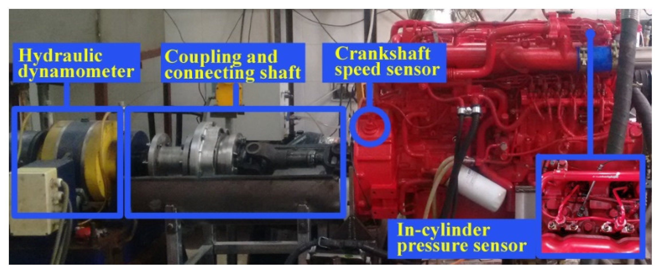
The test engine was a four-stroke, six-cylinder-inline diesel engine. In order to adjust the fuel injection parameter conveniently, a diesel engine with electronic unit pump was employed. In addition, with larger number of cylinders, an engine would operate steady, so the fault features of misfire would become weaker relatively [28]. Thus, a six-cylinder engine was selected. The basic technical data of engine is shown in

Table 1. Engine specifications.

Parameter	Value
Engine type	CY6BG332
Configuration	Six-cylinder, inline, four-stroke
Air intake	Turbocharged, intercooled
Firing order	1-5-3-6-2-4
Fuel injection system	Electronic unit pump
Total displacement	5.95 L
Compression ratio	18.5
Rated power	88 kW @ 2200 r/min
Maximum torque	450 Nm @ 1000–1800 r/min

. A hydraulic dynamometer was connected to the engine for providing external load. A flexible shaft coupling was mounted to connect the engine crank shaft and the dynamometer. Figure 1 shows the picture of the whole test-rig.

A Kistler high-temperature pressure piezoelectric sensor, Type 6058A, was mounted in cylinder 1# through the glow plug hole for verifying misfire occurrence in cylinder chamber. A magnetic sensor, which was mounted opposite to the teeth on the flywheel was used to measure the angular speed of the crankshaft. The sensors’ signals were synchronously sampled and primarily processed using Siemens LMS SCM05 system with 24-bit ADC resolution and a maximum sampling rate of 102.4 kHz.

2.2. Test Description

The measurements were conducted over the engine speed range 800–2200 r/min with interval 100 r/min, at different load levels, as shown in Figure 2. For each engine speed and load value, the measurements were operated under normal, one-cylinder misfire and two-cylinder misfire conditions. The misfire types are shown in

Table 2. All the misfire types.

Categories	Misfire Types
Normal condition	Fault-free
One-cylinder misfire	1#, 2#, 3#, 4#, 5#, 6#
Two-cylinder misfire	Two consecutive cylinders.	1#5#, 3#5#, 3#6#, 2#6#, 2#4#, 1#4#;
	Two cylinders with one-cylinder interval.	1#3#, 5#6#, 2#3#, 4#6#, 1#2#, 4#5#;
	Two cylinders with two-cylinder interval.	1#6#, 3#4#, 2#5#.

. Including normal condition, the total fault types are 22. The misfire condition was achieved by setting the injection parameter zero on the programmable electronic control unit.

The tests were conducted in an intensive engine running speeds and loads, and varied in a wide range. Partial data were used for network training and the rest were used for network testing. The size of training dataset had been set from large to small until an optimal size was achieved.

3. The Speed Characteristics under Misfire and the Limitation of Traditional Misfire Detection Method

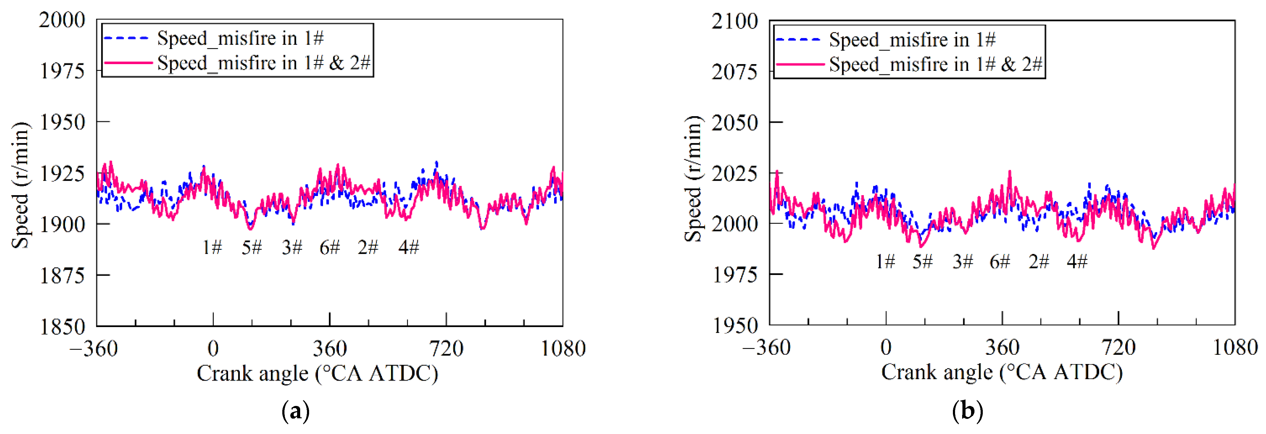
When misfire occurs, the instantaneous engine crankshaft speed will drop and the subsequent speed will rise up compared with the normal conditions. The variation of the whole speed curve will be larger. An example is shown in Figure 3a, under the running condition of 1000 r/min and 100 Nm, when a misfire occurs in cylinder 1#, as the dash curve indicates, the speed becomes different from the normal condition. When the engine speed is high and the load is low, as shown in Figure 3b, the variation rule of instantaneous crankshaft speed becomes unclear, and the difference between normal and misfire condition also becomes indistinguishable. Moreover, when two-cylinder misfire occurs, the fault features expressed from engine speed curve is easily confused with that of one-cylinder misfire condition, especially under the high-speed and low-load conditions. Figure 4a,b show the comparison between speed curves of one-cylinder misfire and two-cylinder misfire.

Therefore, for detecting misfire accurately, the fault features that can reduce or eliminate the interference from engine speed and load should be found. One way to eliminate the impact of engine running range is to divide it into small blocks and then find fault features for each block [27]. However, this will increase workload when the engine running range is large. The better way is to find or design an algorithm that can extract useful feature or can learn more features for the whole engine running conditions.

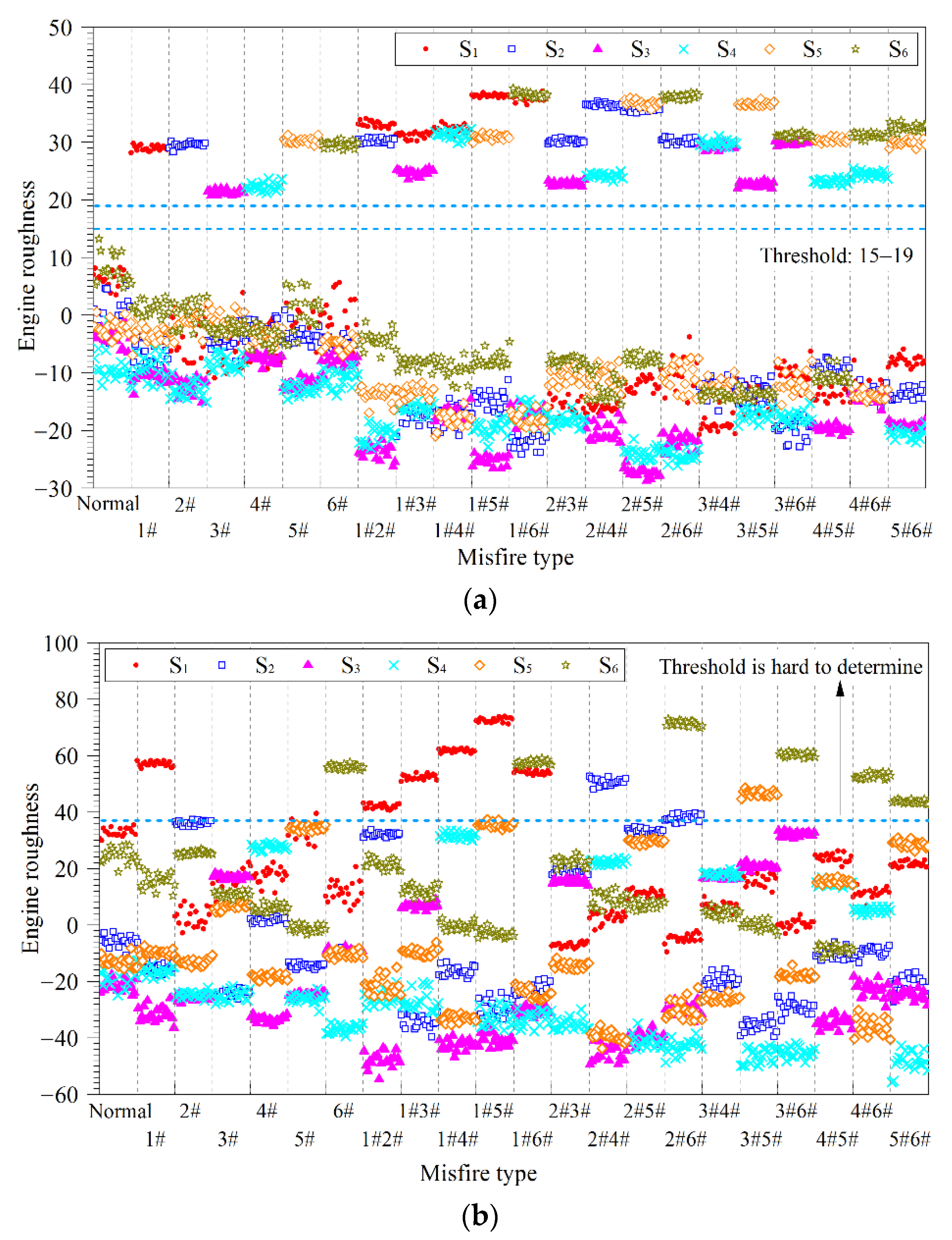
An example of the traditional methods which is called engine roughness method is introduced as below. This method calculates a misfire indicator that is based on the difference of two consecutive angular accelerations. Equation (1) presents the calculation of the indicator [10].

$${\mathrm{S}}_i=\left(T_{i+1}-T_i\right)/T_i^3$$

(1)

where S_i is engine roughness of the ith cylinder. T_i is the time period from ignition of the ith cylinder to ignition of the next cylinder in firing order.

Figure 5 shows the results of indicator S under different engine speeds and different misfire patterns. When misfire occurs in cylinder i, the corresponding S_i will become larger than the predefined threshold. An example is shown in Figure 5a, the threshold can be defined in range 15–19, and when S_i is detected larger than the threshold, it is thought the misfire happened in the cylinder i. This method is limited at the high-speed low-load conditions. As shown in Figure 5b, under 1900 r/min and no-load condition, it is hard to determine the threshold, and the two-cylinder misfire modes are easily confused with one-cylinder misfire modes.

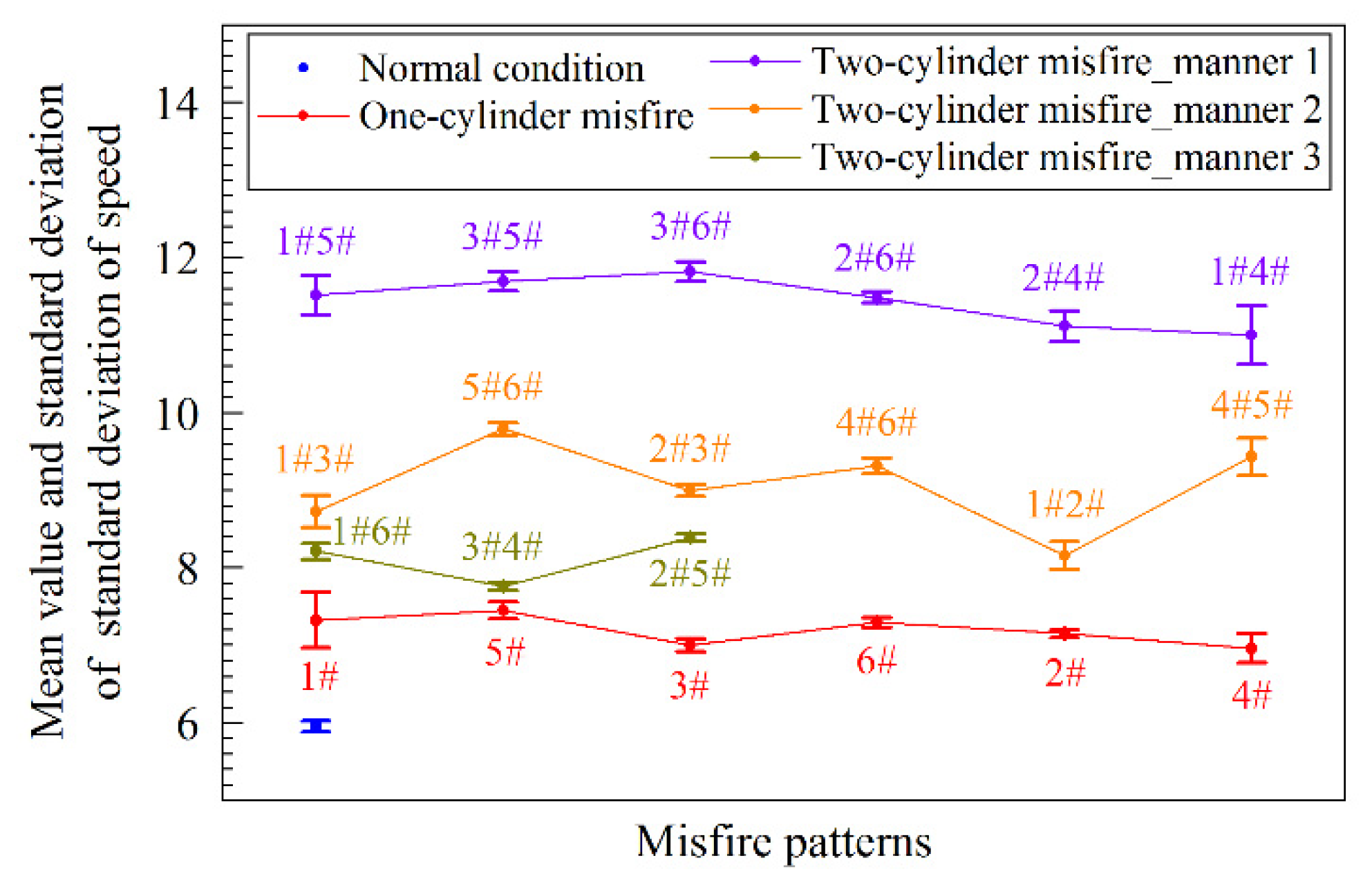
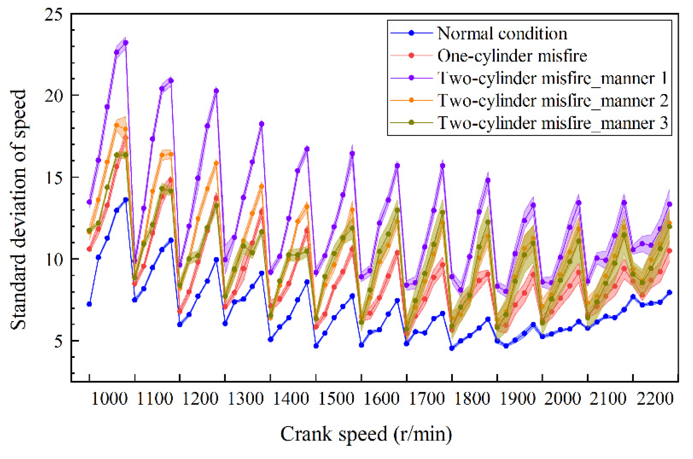
The unsatisfied results appeared at high-speed and low-load conditions are caused by the background noise which has approximately the same order of magnitude with the value related to the misfire presence. The reasons for relatively higher background noise are mainly from the different burning behaviors caused by the systematic nonuniformity. In addition, with the speed increasing and load decreasing, the signal to noise ratio will decrease since the useful features caused by misfire will decrease. Figure 6 presents the standard deviation of crankshaft speed under 800 r/min and no-load conditions. The standard deviation is calculated once per cycle, the points in Figure 6 which are shown in the form of mean value and standard deviation are calculated from 200 cycles of data. The results clearly show that when misfire occurs, the amplitude of speed variation will increase, and this is helpful for extracting misfire features. However, when engine speed becomes higher and load becomes lower, the amplitude of speed variation decreases, and the amplitude difference between normal and misfire patterns also decreases, as shown in Figure 7. Then, the signal to noise ratio decreases. The limitation of the engine roughness method proves that it is hard to use too few features to achieve a perfect fault detection result.

Since LSTM RNN is good at learning features of sequences, the LSTM RNN is utilized in this paper to detect misfire and to overcome the limitation of traditional algorithm.

4. The LSTM RNN

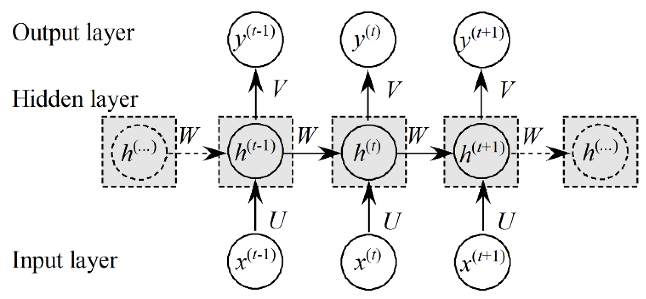
The classical artificial neural networks are design to extract features from datasets whose sub-samples are independent with each other. In some application scenarios, like natural language processing, the meaning of a whole sentence is dependent on the meaning and order of the previous and later words. RNNs are designed to be applied in this kind of research field. RNNs are connectionist models that capture the meaning of sequences via cycles in the network. Basic architecture of an RNN is shown in Figure 8, which is an unfold architecture.

As presented in Figure 8, the forward pass of an RNN module looks the same as that of a multi-layer perceptron which has a single hidden layer. The main difference is that the activations of the hidden layer are from both the current input layer and the hidden layer activations from the previous step, as described in Equation (2) [29]. Equation (3) calculates the output value or vector. Thus, an RNN will map the input sequences into output.

$$h^{(t)}=f\left(b+W{h}^{(t-1)}+U{x}^{(t)}\right)$$

(2)

$$y^{(t)}=V{h}^{(t)}$$

(3)

where W, U and V are the weight matrices. b, x, h, f, and y donate the bias vector, input vector, hidden layer vector, activation function and the output vector, respectively.

The classic RNN has the problem of a vanishing gradient [30]. In addition, sometimes gradient explosion will also occur. This is because the error surface is either very flat or very deep after updating weights in many time steps. This problem is also called the long-term dependency problem. One effective way to solve this problem is using gating mechanism to control the information passing path, such as LSTM.

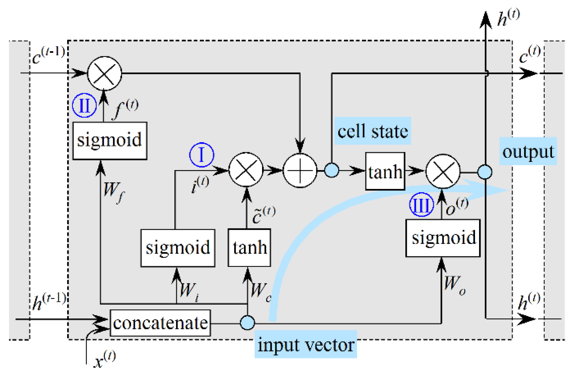
LSTM RNN has the basic structure of RNN, which is a chain of repeating modules. The main difference of an LSTM RNN from other RNNs is the structure of the module, which is marked with shadow area in Figure 8 and Figure 9. In a module of LSTM RNN, three gates are designed to control the output.

The main line of an LSTM module is the calculations of input vector, cell state and output, as indicated by the blue dot and arrow in Figure 9. First of all, the input vector of LSTM module is acquired by concatenating the outputs of the previous module and the current inputs. Secondly, two gates are designed to adjust the cell state. As shown in Figure 9, the input gate is applied to decide whether the current inputs will be used to update the cell state. By the same principle, the forget gate is applied to adjust the proportion of previous cell state in the current one. This makes an LSTM module have the memory function. Then the cell state will be updated and stored for the LSTM module of next step. Next, an output gate is designed to adjust the output of the updated cell which has been rescaled by a tanh activation function firstly. Finally, the output will be transported to the next layer and the next module.

Equations (4) and (5) show the calculation of new candidate vector ${\tilde{c}}^{(t)}$ and input gate vector $i^{(t)}$; Equation (6) calculates the forget gate vector $f^{(t)}$; the cell state $c^{(t)}$ can be updated by Equation (7); the output gate vector $o^{(t)}$ is calculated by Equation (8); and the final output $h^{(t)}$ will be acquired by Equation (9) [24]. The output vectors of these three gates are all the values between 1 and 0, which will make the outputs of corresponding layer change from original value to 0.

$${\tilde{c}}^{(t)}=\tanh \left(W_c\cdot [h^{(t-1)},x^{(t)}]+b_c\right)$$

(4)

$$i^{(t)}=\mathrm{sigmoid}\left(W_i\cdot [h^{(t-1)},x^{(t)}]+b_i\right)$$

(5)

$$f^{(t)}=\mathrm{sigmoid}\left(W_f\cdot [h^{(t-1)},x^{(t)}]+b_f\right)$$

(6)

$$c^{(t)}=f^{(t)}\circ c^{(t-1)}+i^{(t)}\circ {\tilde{c}}^{(t)}$$

(7)

$$o^{(t)}=\mathrm{sigmoid}\left(W_o[h^{(t-1)},x^{(t)}]+b_o\right)$$

(8)

$$h^{(t)}=o^{(t)}\circ \tanh (c^{(t)})$$

(9)

where sigmoid and tanh are activation functions. $x^{(t)}$ is the input vector from training or testing dataset. $h^{(t-1)}$ and $h^{(t)}$ are the current and previous outputs of LSTM module, respectively. $[h^{(t-1)},x^{(t)}]$ means concatenating $h^{(t-1)}$ and $x^{(t)}$. $b_c$, $b_i$, $b_f$, and $b_o$ are biases. $W_c$, $W_i$, $W_f$, and $W_o$ are weight matrices. $\circ$ means Hadamard product. When the network is trained, $b_c$, $b_i$, $b_f$, and $b_o$ are initialized with ones. For $W_c$, $W_i$, $W_f$, and $W_o$, each weight matrix is the concatenation of two matrices which are corresponding to $h^{(t-1)}$ and $x^{(t)}$, respectively; accordingly, the two parts of a weight matrix are initialized, respectively. In this work, both the two parts of each weight are initialized as uniform distribution which is shown in Equation (10) [31].

$$W\sim U\left[-\frac{\sqrt{6}}{\sqrt{n_j+n_{j+1}}},\frac{\sqrt{6}}{\sqrt{n_j+n_{j+1}}}\right]$$

(10)

where $n_j$ and $n_{j+1}$ is the element number layer j and j + 1, respectively.

This is the key mechanism of LSTM RNN. The network training is also based on back propagation through time (BPTT) strategy and gradient descent algorithm. Up to now, there have been many types of variants on the LSTM, such as adding peephole connections, using coupled forget and input gates, gated recurrent unit, depth gated RNNs and so on. As reported in Greff’s work [32], the result of comparing these popular LSTM variants shown that there were not significant differences among them. Therefore, the standard LSTM RNN is adopted in this paper.

5. Signal Processing and Results Analysis

5.1. Network Training Strategy

The experiments have been described in Section 2.2. There are 70 different engine running speeds and loads conditions in total. For each condition, 22 misfire types were conducted. Under each fixed speed, load and misfire type condition, 200 cycles data were sampled. Thus, the number of total datasets is 308,000 (22 × 70 × 200 = 308,000), and one dataset corresponds to one engine power cycle which contains 120 speed data point.

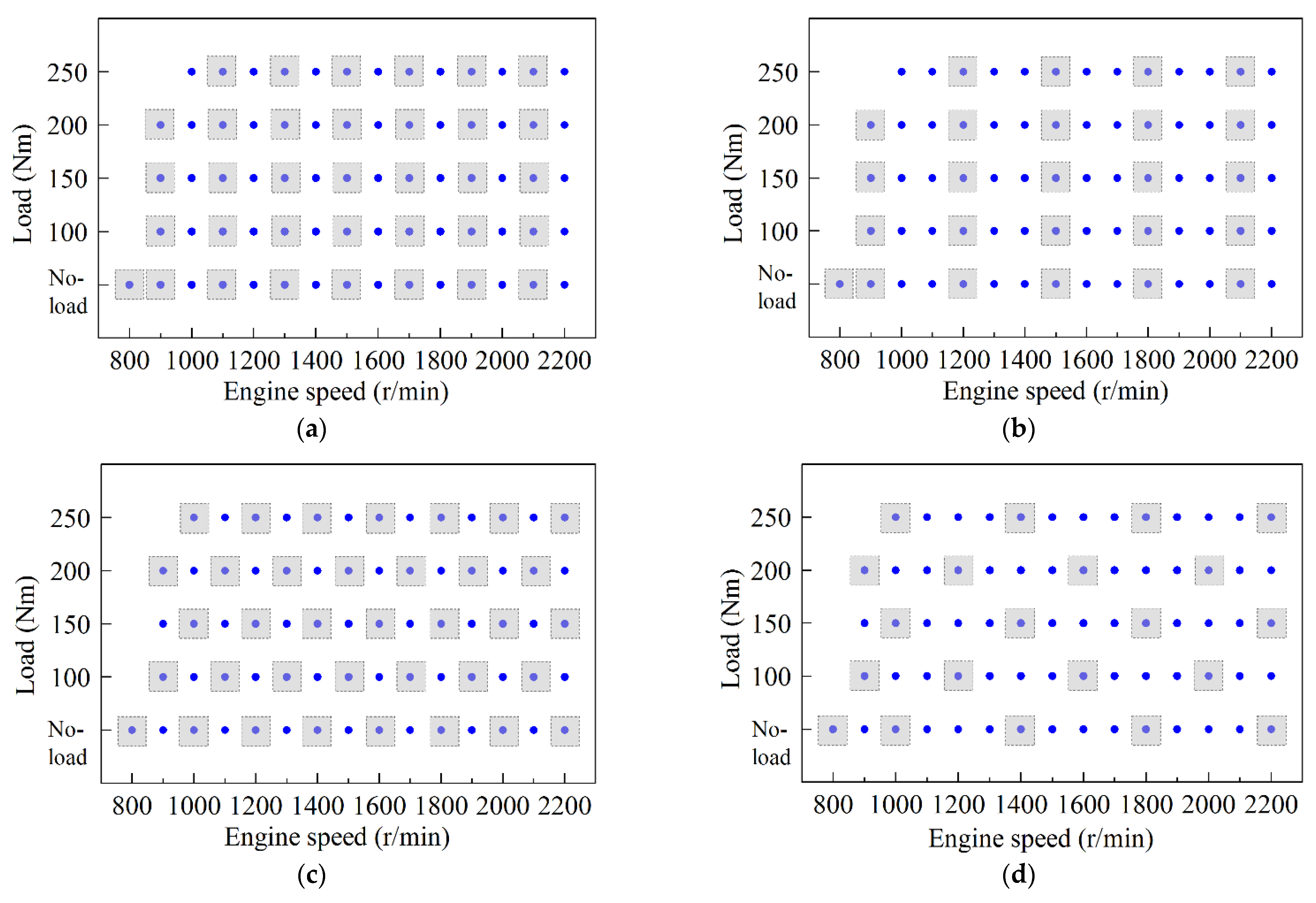
The datasets were acquired in a dense speed and load range. However, for industrial application, it would be better to use small number of datasets to train a well-performed neural network. Five division modes of training and testing datasets were attempted, as described in

Table 3. Description of the training and testing datasets arrangement.

	Description
Mode 1	All the datasets are arrange randomly, then 70% datasets are chosen for network training and the rest for network testing.
Mode 2_a	As shown in Figure 10a.
Mode 2_b	As shown in Figure 10b.
Mode 2_c	As shown in Figure 10c.
Mode 2_d	As shown in Figure 10d.

. The arrangement of mode 1 will be attempted firstly, and if the test result is higher than 90%, the rest arrangements will be tested. The arrangements of modes 2_a, 2_b, 2_c, and 2_d are shown in Figure 10, in which the training datasets are the conditions in shadow, the rest datasets are for testing. The arrangements in Figure 10a, c will be attempted first, and if the test results are higher than 90%, the arrangements in Figure 10b,d will be tested.

In order to achieve a better performance of the LSTM RNN, four different structures of input layer and output layer have been tested.

• The first structure takes the original speed sequence as input. As shown in Figure 11a, one LSTM cell has one input element and one output element. For each engine cycle there are 120 speed points, and 120 output elements correspondingly. The output types are the normal and misfire types in Table 2.
• For the second structure, inputs are the same as those in the first structure. For each cycle, there is only one output element at the last LSTM cell. As shown in Figure 11b, when the 120 input elements have been calculated, one detection result will be output. The output types are the normal and misfire types in Table 2.
• In the third structure, one LSTM cell processes 20 raw speed points which correspond to the interval of ignition from one cylinder to the next. As shown in Figure 11c, the output of one LSTM cell consists of two categories: normal and misfire, which is different from those in the first and second structures.
• The inputs of the fourth structure are not the raw speed data, but the lowest 20 real and 20 imaginary parts of the frequency-domain results of instantaneous speed, as shown in Figure 11d. The output types are the normal and misfire types in Table 2.

The basic parameters for these four types of networks are summarized in

Table 4. The basic parameters of networks utilized.

	The 1st Network	The 2nd Network	The 3rd Network	The 4th Network
Preprocessing	None	None	None	Fourier synchrosqueezed transform
Input mode of LSTM	Sequence	Sequence	Sequence	Sequence
Input size	1	1	20	40
Dimensionality of LSTM cell state (Number of hidden layer elements)	20	3, 5, 10, 20, 40, 80	3, 5, 10, 20, 40, 80	3, 5, 10, 20, 40, 80
Output mode of LSTM	Sequence	Last	Sequence	Sequence
Output size of fully connected layer	22	22	2	22
Postprocessing	None	None	Combining per cycle	None

.

5.2. Results Analysis

5.2.1. The First Network Structure

For the first structure which is designed as Figure 11a, one input group consists of 10 datasets, that is 1200 (120 × 10) speed data points. One output group has the same length with the corresponding input. The network consists of one input layer, one LSTM layer, and one output layer. The initial learn rate is 0.01 and the learn rate drop period is 3. The adaptive moment estimation method is adopted for network training. The number of elements of hidden layer is 20. When the training and testing datasets are arranged as mode 1, the final training and testing accuracies are 17.35% and 15.36%, respectively. Since the accuracies are not high, no more tests are attempted.

5.2.2. The Second Network Structure

The second structure is designed as Figure 11b. One input group consists of one dataset which is 120 speed data points. Only the last LSTM cell outputs prediction result. The network consists of one input layer, one LSTM layer, and one output layer. The initial learn rate, the learn rate drop period, and the training algorithm are the same as those in the first structure.

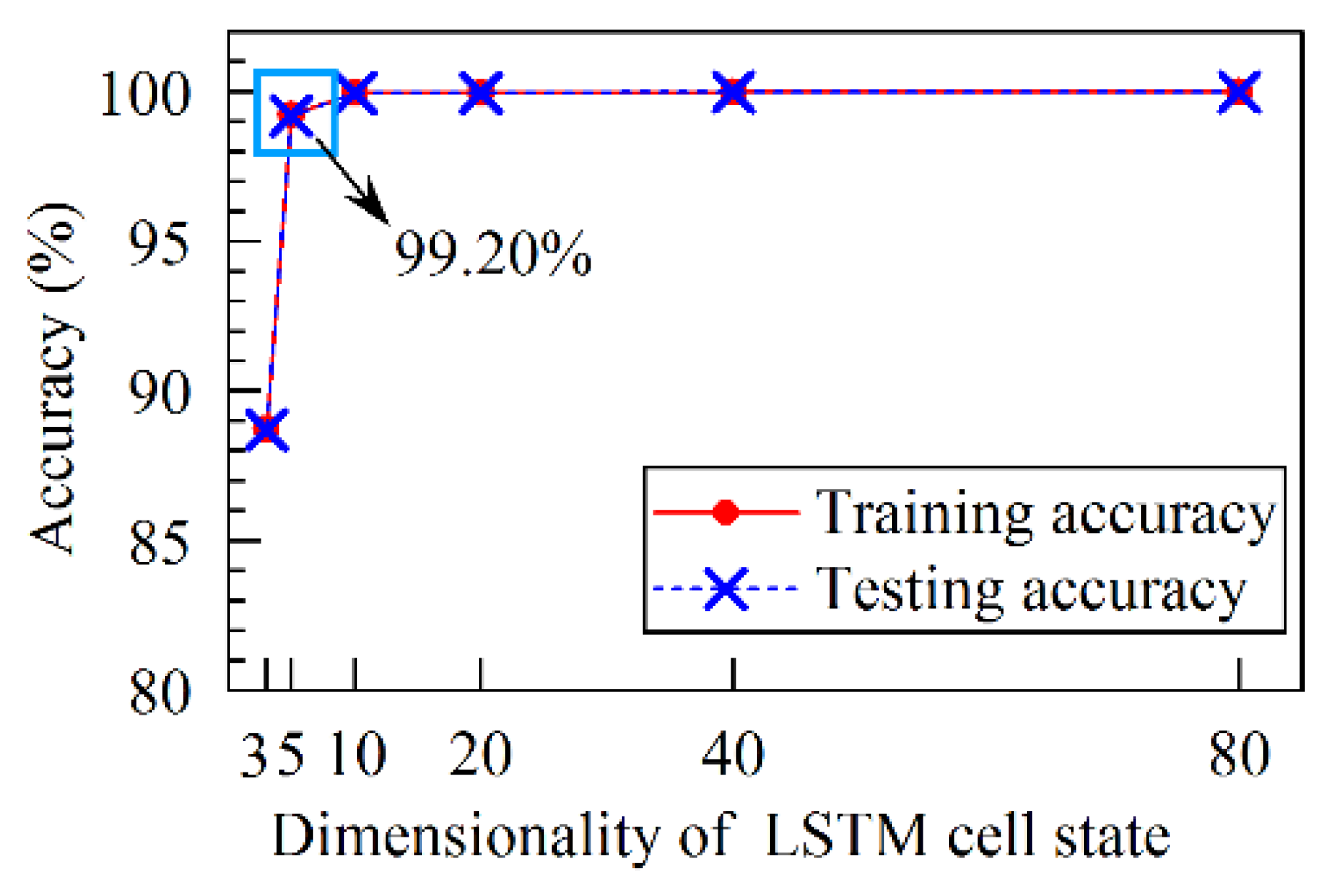
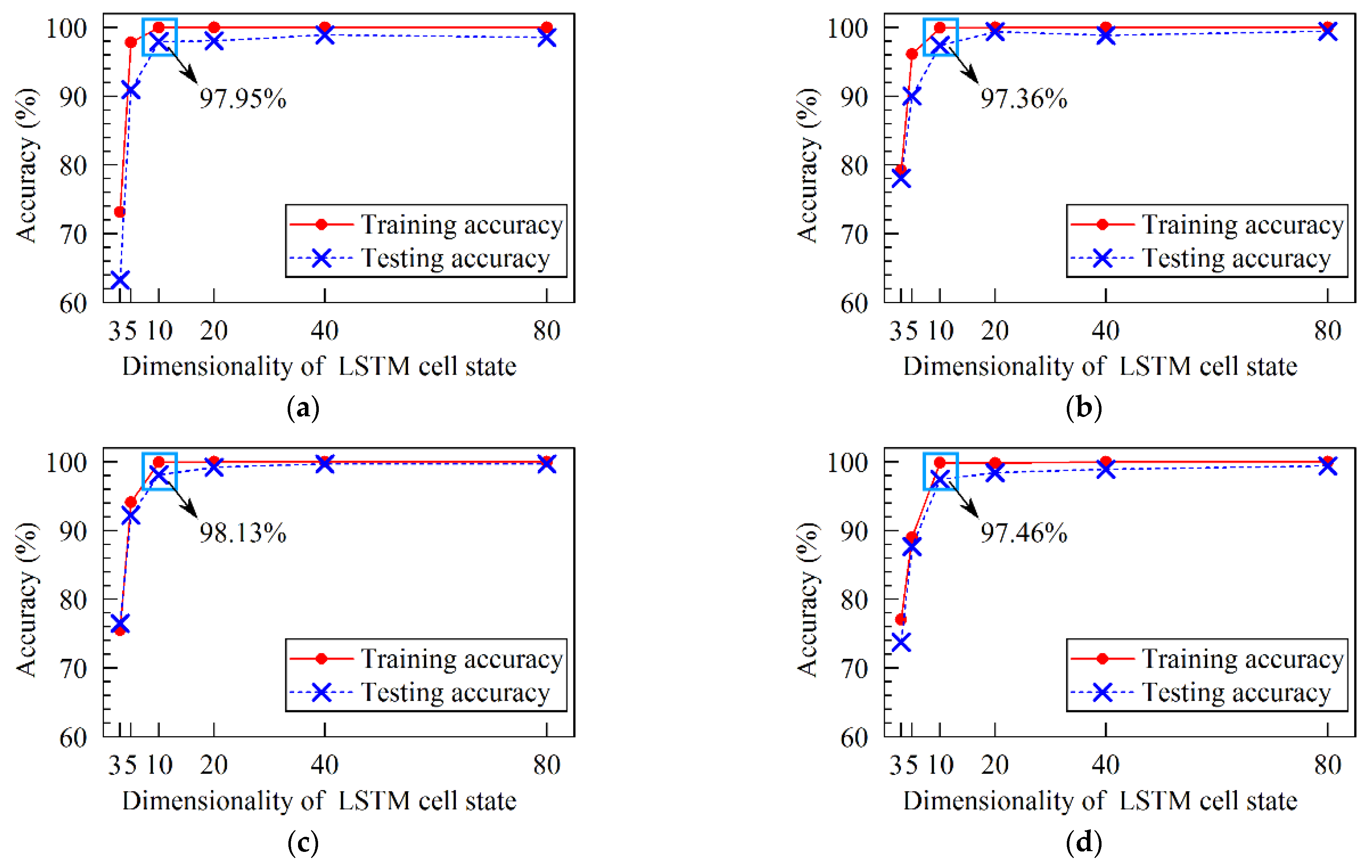
When the training and testing datasets are arranged as mode 1 (described in Table 3), the element numbers of LSTM layer, which are 3, 5, 10, 20, 40 and 80, have been tested. The corresponding training and testing accuracies are drawn in Figure 12. It is thus clear that when the training datasets are arranged as mode 1, 5 elements are enough for the network training, and the corresponding training and testing accuracies are 99.23% and 99.20%. Since the accuracies are very high, the datasets arranged in modes 2_a, 2_b, 2_c and 2_d are tested and the results are shown in Figure 13. It can be seen that utilizing the training datasets in a sparser manner, the acceptable performance can also be acquired. It seems that with less training data, it will be easier to train a network that can achieve the accuracy higher than 95%, such as the network trained in modes 2_b and 2_d.

5.2.3. The Third Network Structure

The third structure is designed as Figure 11c. One input layer consists of 20 elements which correspond to the interval of one-cylinder working. The output of one LSTM cell consists of two categories which are normal and misfire, and each LSTM cell has a corresponding output. The output indicates whether the current powering cylinder is fault-free. The initial learn rate, the learn rate drop period, and the training algorithm are the same as those in the first method.

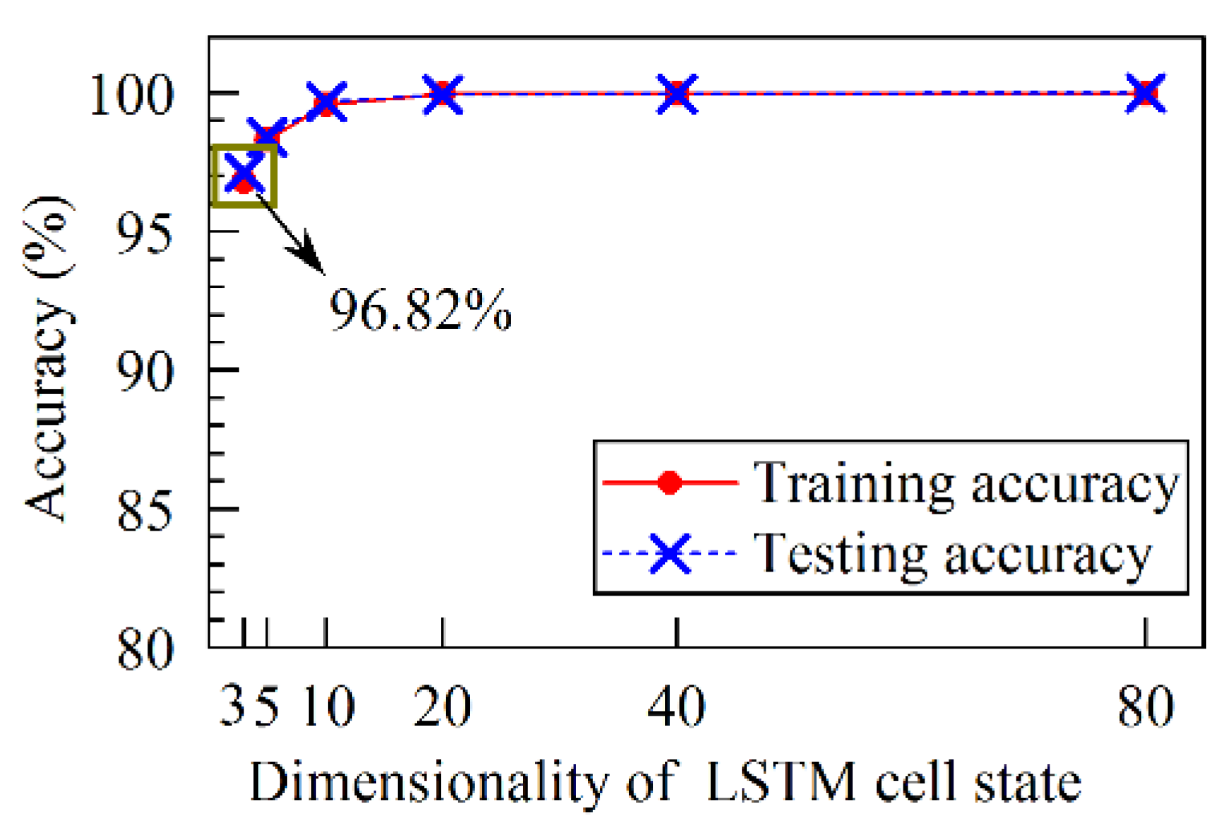
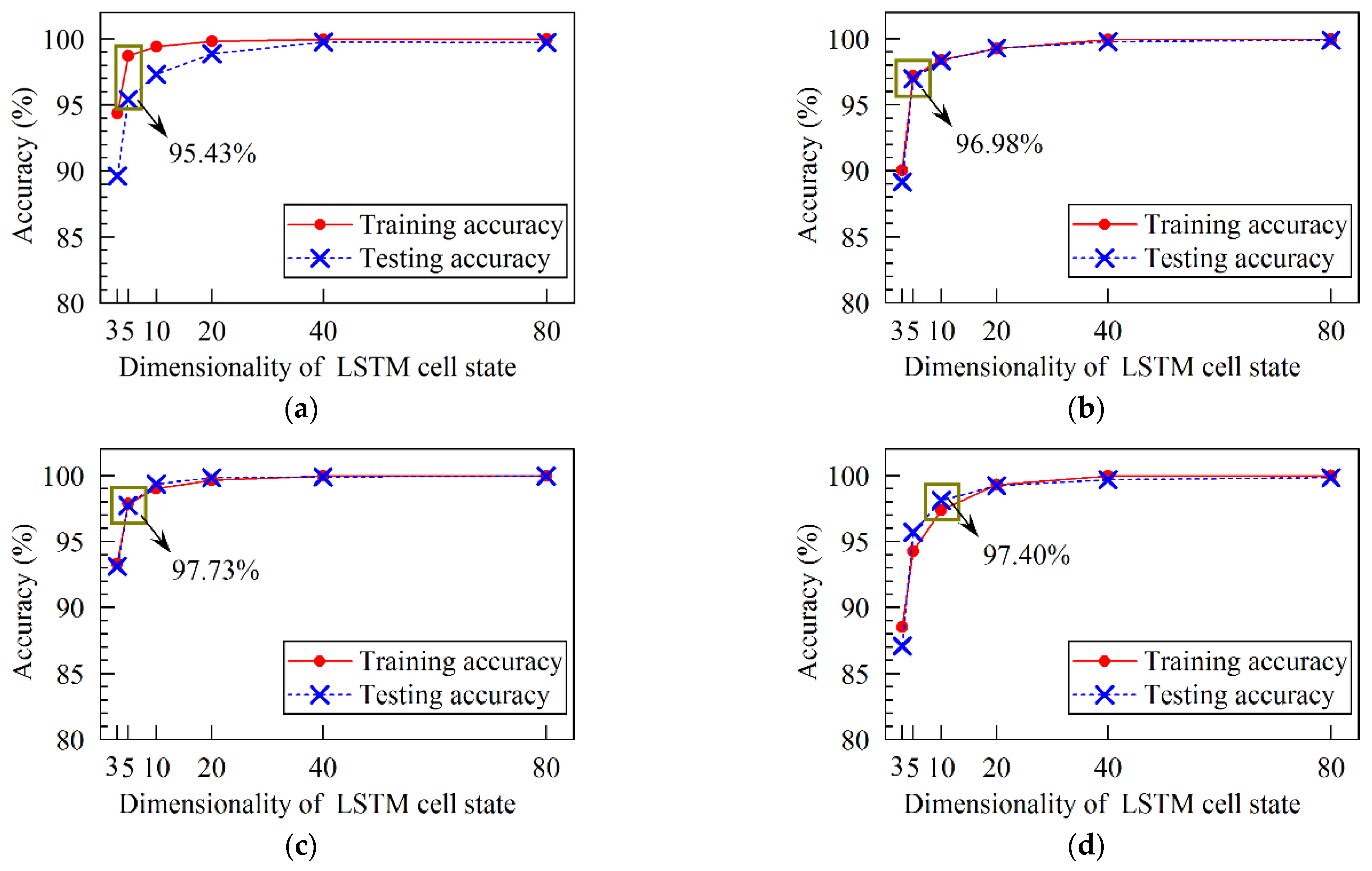
The training and testing datasets are arranged as Table 3. The training strategy is also by changing the numbers of hidden layer elements, which are 3, 5, 10, 20, 40 and 80. The training and testing results under mode 1 are summarized in Figure 14. The training and testing results under modes 2_a, 2_b, 2_c, and 2_d are summarized in Figure 15. Since the outputs are calculated for each cylinder, it is unable to compare the original results with other methods. Therefore, when we calculate the accuracy, the results for one cylinder are converted to that for one cycle. The concrete method is to group every six consecutive outputs from cylinder 1# and tag each group according to the fault cylinders. If three or more fault cylinders are detected in one cycle, the result will be categorized as a fault prediction. Compared with the second network structure, the third network structure has higher accuracy with the same number of hidden layer elements. For most of the five data division modes, 95% accuracy can be achieved with no more than 5 hidden layer elements.

5.2.4. The Fourth Network Structure

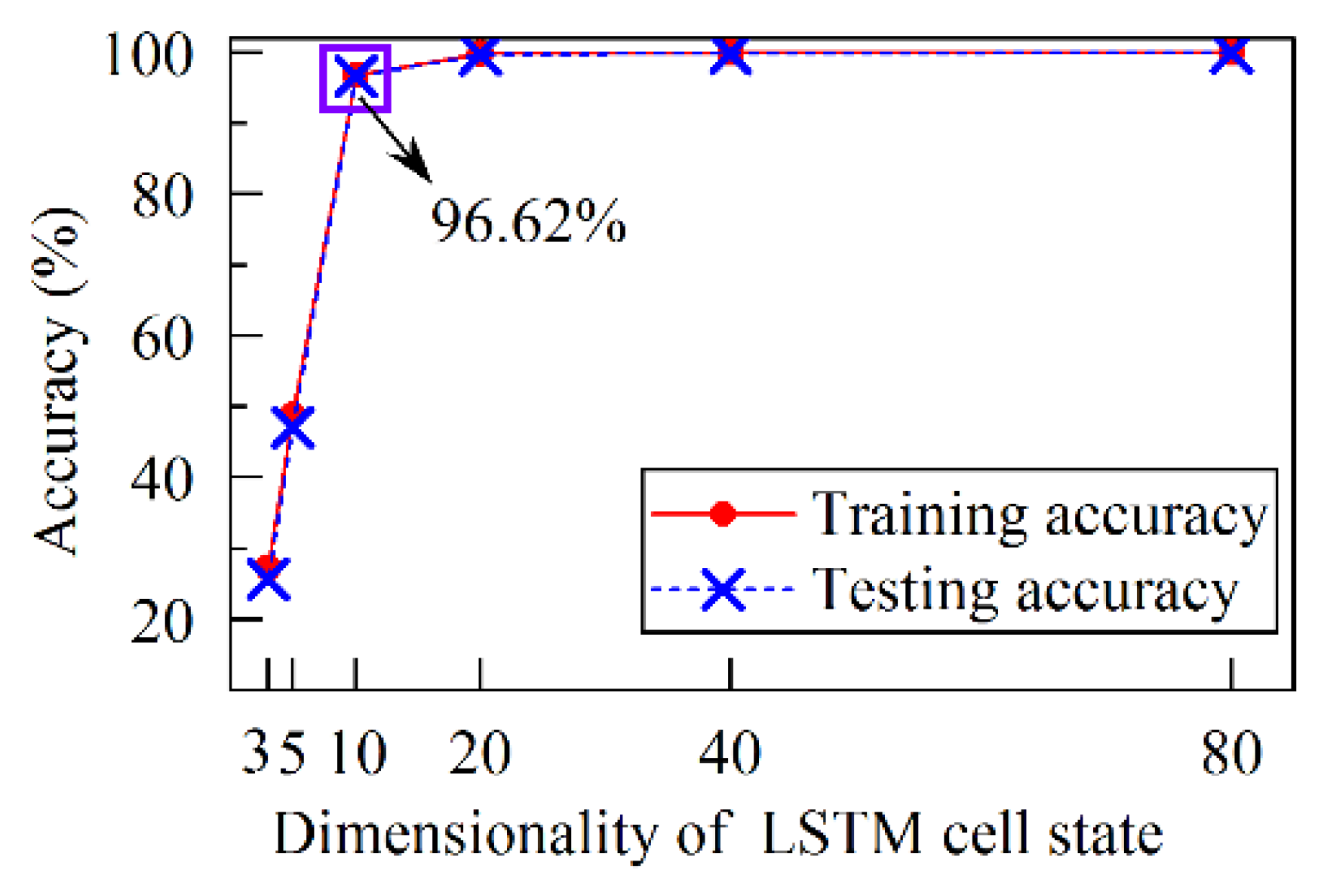
The fourth structure is designed as Figure 11d. One input layer consists of 40 elements which are the lowest 20 real and 20 imaginary parts of the frequency-domain results of the speed signal. For the normalization of inputs, the 20 real parts and the 20 imaginary parts are normalized, respectively. The frequency-domain results are acquired by transforming the raw speed using Fourier synchrosqueezed transform algorithm [33]. As a type of time-frequency analysis method, the Fourier synchrosqueezed transform algorithm could acquire the instantaneous frequency-domain information more precisely than short-time Fourier transform. This advantage is helpful for abstracting fault features from the speed signal. Since there are 60 teeth of the flywheel, the sample rate is set as 60. The data length of one cycle is 120, and the data length of 2’s power could achieve high computational speed; thus, the truncated data length is set as 128. A Kaiser window is utilized for reducing spectral leakage. Considering that the output is in the manner of sequence which means each LSTM cell has an output, the accuracy is calculated according to the last output of one cycle. Figure 16 and Figure 17 present the training and testing results using the fourth structure.

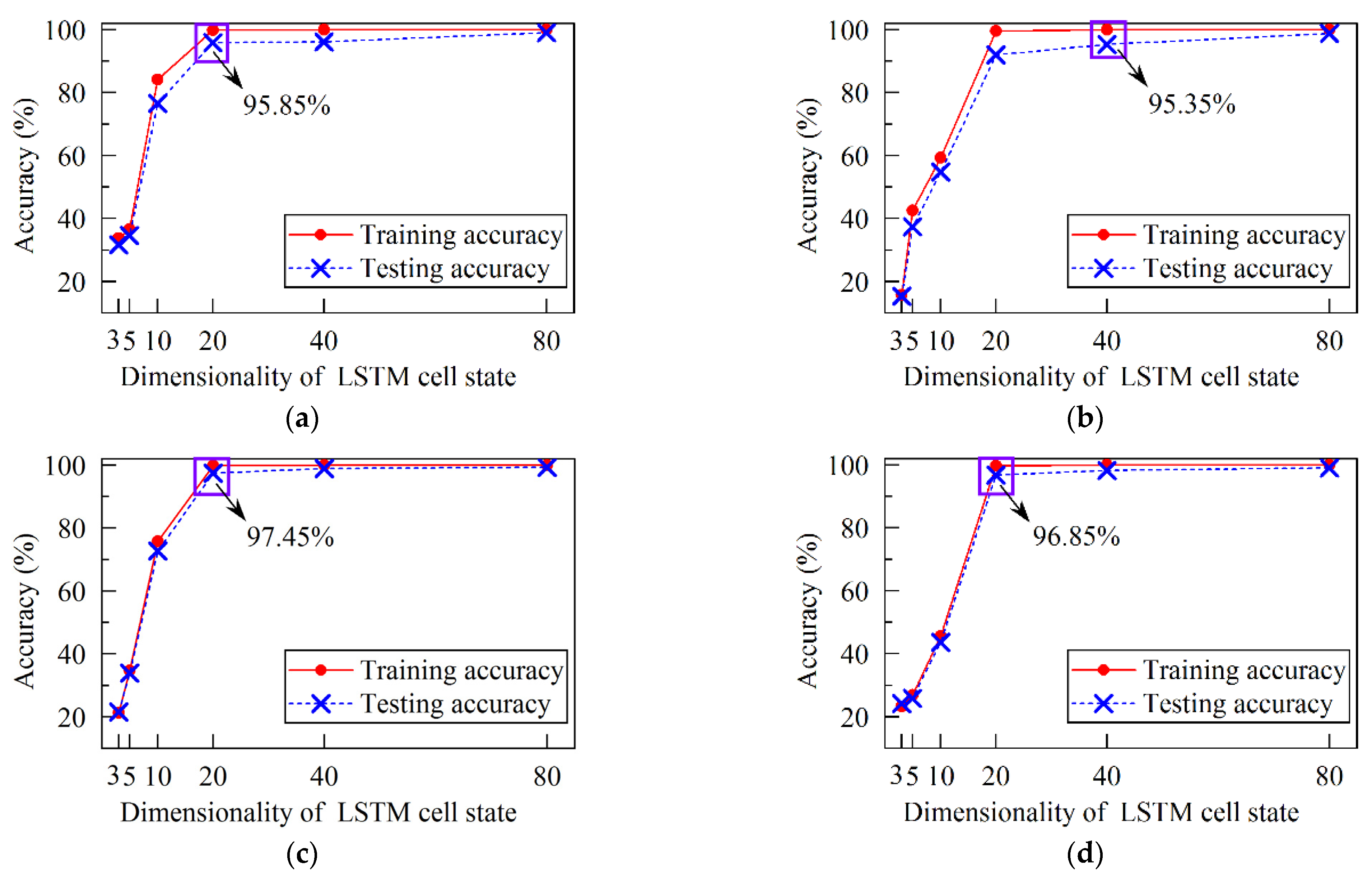
Like the previous methods, the main variables are also the data division mode and the number of hidden layer elements. The results show that it is easy to achieve high accuracies which are more than 95% when the training data and testing data are arranged in mode 1. However, when the data are arranged as modes 2_a, 2_b, 2_c and 2_d, 20 or more hidden layer elements are needed for achieving 95% accuracy.

5.2.5. Results Comparison

(a)

Through the above analysis, it is known that it acceptable training and testing accuracies can be achieved by using LSTM RNN.

(b)

Compared with other network structures, the first network structure cannot achieve a satisfactory accuracy and is not studied further. The second, third and fourth network structures can achieve an accuracy which is more than 95%.

(c)

From the point of view of data division mode, under mode 1, the second, third and fourth network structures can achieve accuracy more than 95%. The performance of these three structures is good, since 10 hidden layer elements have made them meet requirements and even 3 elements are enough for the third network. Under modes 2_a, 2_b, 2_c, and 2_d, the training and testing datasets are divided in the rule that they have no intersection on engine speed and load conditions. Under these four modes, even all the three methods could achieve accuracy more than 95%, to our minds, the third method performed the best since it could reach 95% accuracy with the least number of hidden layer elements.

(d)

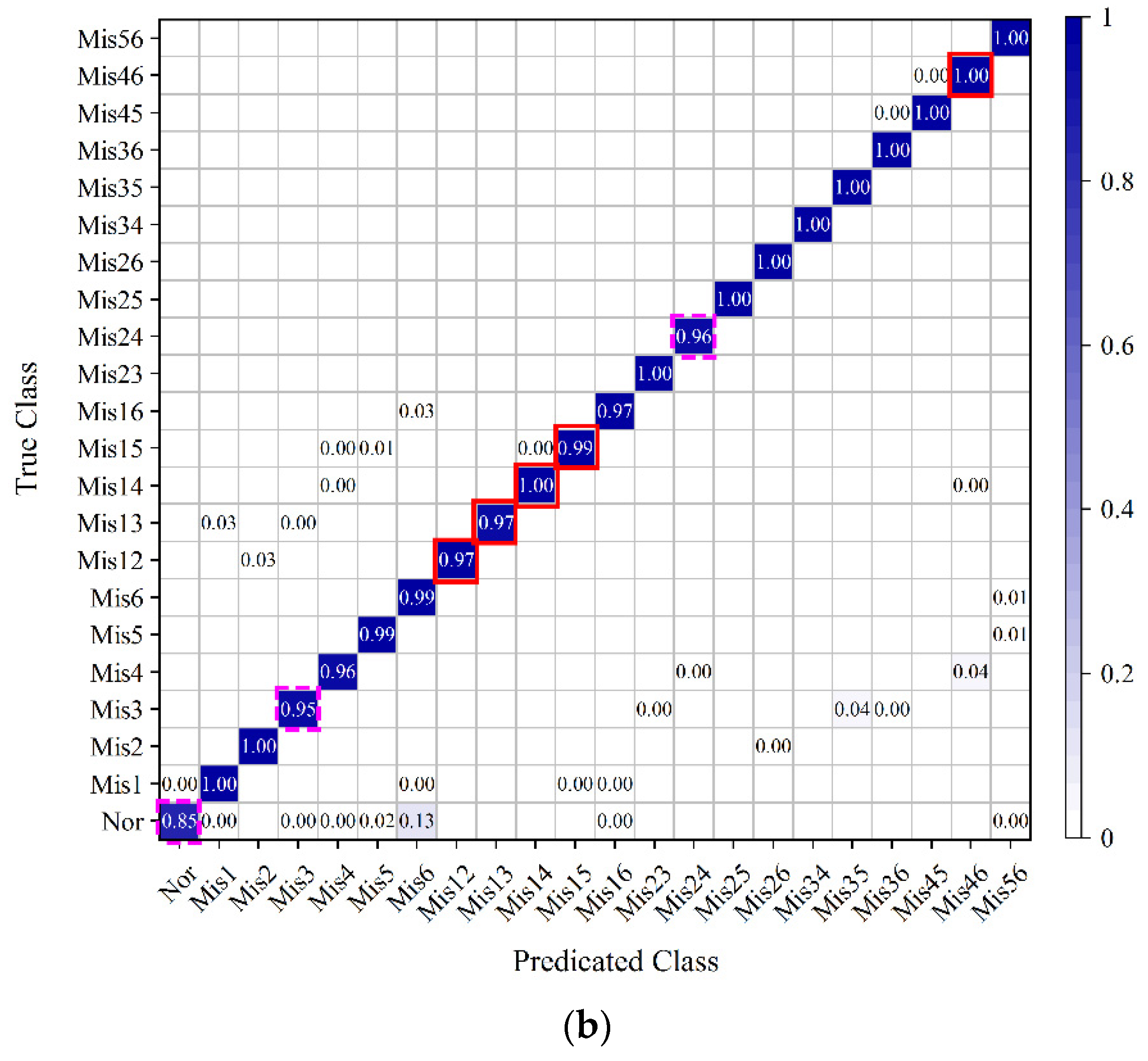
In addition, when we tested the third network on data division mode 2_d with 5 and 10 hidden layer elements, it was found that the testing accuracy was higher than the training accuracy, as shown in Figure 15d. Taking the network structure with 10 hidden layer elements as an example, the confusion matrices are shown in Figure 18. The main increase of testing accuracies is marked by red boxes. It can be seen that many accuracies have increased to more than 95%. The increment may be caused by the testing data that belongs to the same fault category with the training data, but is sampled under different engine running speed or load. The network with 5 or 10 hidden layer elements just grasped the fault features of the training data unevenly. Therefore, the increase of total accuracy can be seen as a random result. However, the detection accuracy on the normal condition has decreased to 85%. Since the learning ability of network is determined when the network structure is determined, if there happened some excellent results on partial conditions, there must be some bad results correspondingly. The difference between excellent and bad results may be big or small, even the total accuracies are almost the same. In this case, the bad results occurred on the normal conditions. The accuracy of 85% is unacceptable on one hand, on the other hand, the misdiagnosis should be avoided on normal conditions since the normal conditions are the most common conditions for a vehicle. The results also indicate that both the total accuracy and the accuracy of each fault category should be acceptable especially under the condition of large datasets.

(e)

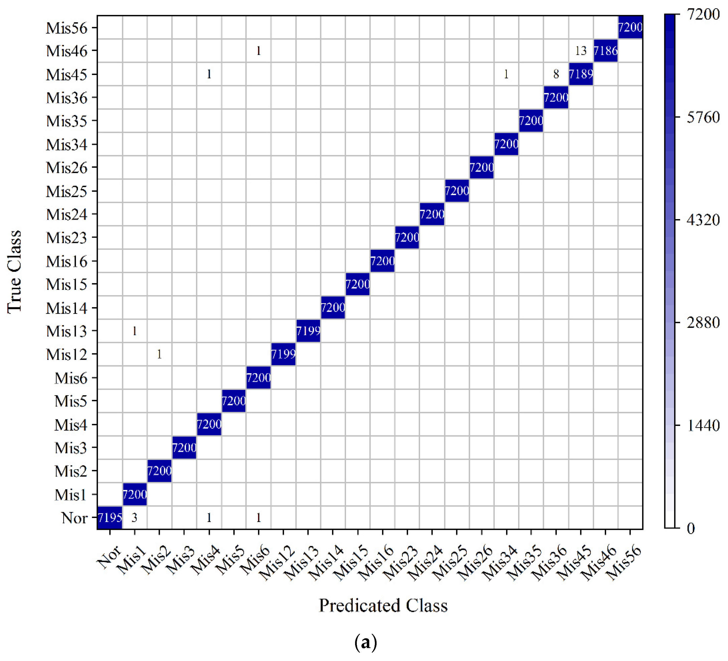
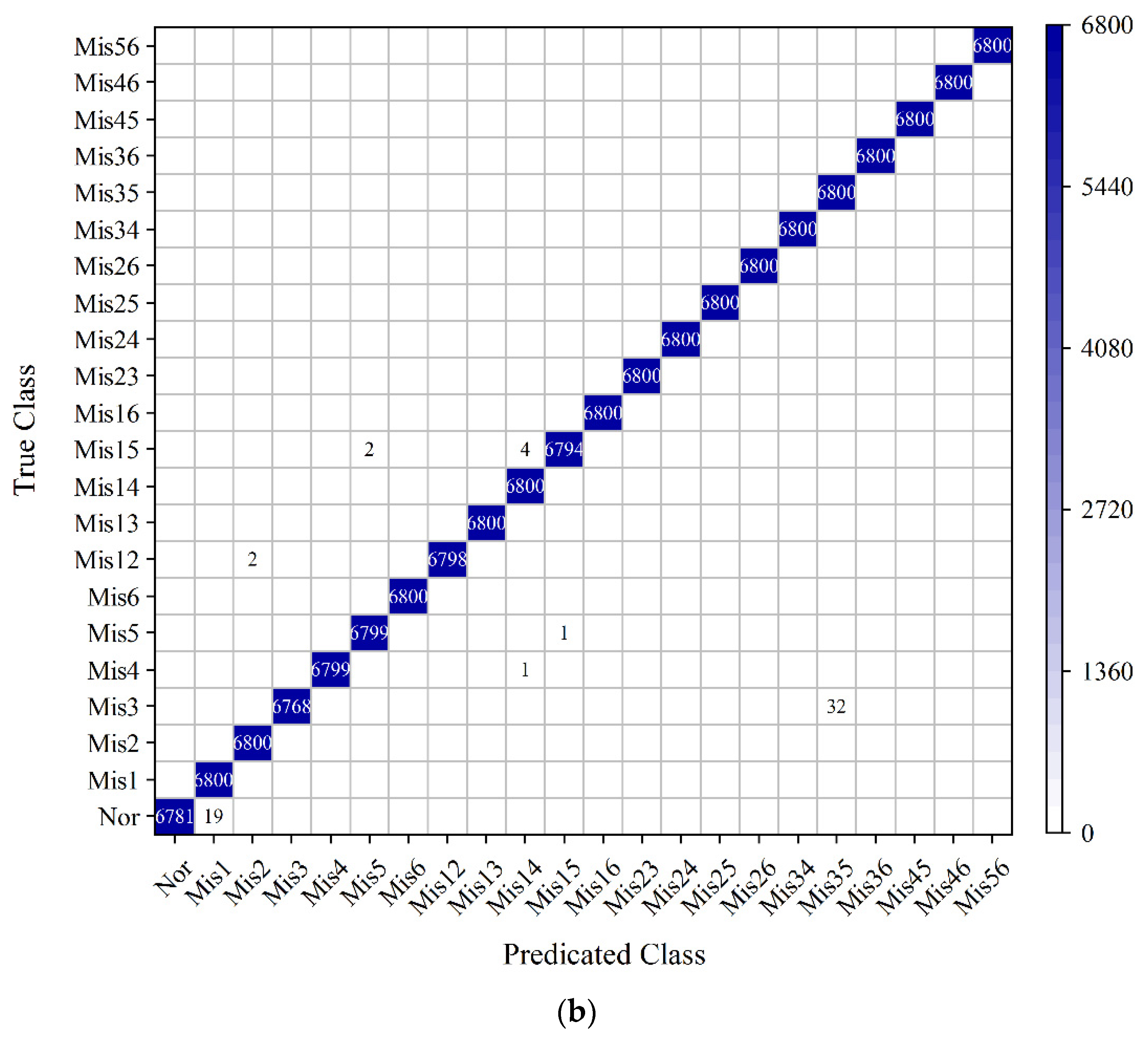
In industrial applications, the smaller training dataset would be better for reducing workload for a calibration engineer. The best performance of the second, third and fourth networks under modes 2_a, 2_b, 2_c, and 2_d are summarized in

Table 5. The best accuracies for different networks under different data division modes.

	Mode 2_a (%)		Mode 2_b (%)		Mode 2_c (%)		Mode 2_d (%)
The second network	99.99	98.93	99.98	99.44	99.99	99.69	100	99.37
The third network	99.98	99.76	99.95	99.90	99.98	99.96	99.99	99.83
The fourth network	99.99	99.14	99.97	98.83	99.97	99.33	100	99.06

For each mode, the left column is training accuracy, the right column is testing accuracy.

. These accuracies are acquired with 40 or 80 hidden layer elements. By comparing the testing accuracies, the third network performs the best. Nevertheless, the difference between each network and each data division mode are not large. Both the training data size and the testing accuracy are the factors we considered, thus the third networks with data division mode 2_b and data division mode 2_c are recommended, and the numbers of hidden layer elements are 80 both. For further analysis, the confusion matrices of the training and testing results are drawn in Figure 19 and Figure 20. Some conclusions can be drawn as follows.

• It can be seen that the distribution of misdiagnosed results is scattered. The number of most misdiagnosed results do not exceed 10.
• In Figure 19, the main misdiagnosis results occur on normal, cylinder 3# misfire, cylinders 1# and 3# misfire, cylinders 4# and 5# misfire, and cylinders 4# and 6# misfire conditions. In Figure 20, the main misdiagnosis results occur on normal, cylinder 3# misfire, cylinders 4# and 5# misfire, and cylinders 4# and 6# misfire conditions. The misdiagnosed results are related to the true results, for example, when misfire occurs in cylinder 3#, the predicted result is misfire in cylinders 3# and 5#.
• The most common running condition for an engine is normal condition. By observing the results in Figure 19 and Figure 20, the worse misdiagnosed case is for normal condition which is presented in Figure 19b. However, the detection accuracy on this normal condition is 98.91% (8902 ÷ 9000 = 98.91%), which is a relatively high detection accuracy. Meanwhile, since the network performs well on the worst misdiagnosis case, it can be concluded that the detecting accuracy for each type of fault is acceptable.

5.3. Comparison with Similar Research Efforts in the Literature

Table 6. Comparison of our results with the similar works in the literature.

Similar Works	Details
Qin et al. [1]	Engine type: four-cylinder diesel engine
	Signal: vibration
	Speed: 1300 r/min, 1800 r/min, 2200 r/min
	Load (Nm): not mentioned
	Misfire type: 1#, 2#, 3#, 4#, 1#2#, 2#3#, 2#4#
	Methods: a deep twin convolutional neural network
	Accuracy: >97.019%
Jafarian et al. [21]	Engine type: four-cylinder engine
	Signal: vibration
	Speed: 2000 r/min
	Load (Nm): not mentioned
	Misfire type: 1#, 2#, 1#2#
	Methods: FFT for feature extraction; ANN, SVM, and kNN for classification
	Accuracy: >97%
Moosavian et al. [19]	Engine type: four-cylinder gasoline engine
	Signal: vibration, sound
	Speed: idle speed (867 r/min)
	Load (Nm): no load
	Misfire type: 1#, 2#
	Methods: wavelet denoising, ANN, least square support vector machine, Dempster–Shafer evidence
	Accuracy: 98.56%
Jung et al. [16]	Engine type: six-cylinder engine
	Signal: crank speed
	Speed: 500–4500 r/min, (step is 500 r/min)
	Load (Nm): not mentioned
	Misfire type: 1#, 2#, 3#, 4#, 5#, 6#
	Methods: model-based algorithm
	Accuracy: no quantitative result. The algorithm performs well except low load and speed conditions.
Zheng et al. [5]	Engine type: four-cylinder gasoline engine
	Signal: crank speed
	Speed: 800–1150 r/min
	Load: not mentioned
	Misfire type: 1#, 2#, 3#, 4#, 1#3#, 2#4#, 1#4#, 2#3#
	Methods: state observer for combustion torque estimation; ANN for classification
	Accuracy: >52/54 (96.30%)
Boudaghi et al. [34]	Engine type: four-cylinder gasoline engine
	Signal: crank speed
	Speed: 1250–4000 r/min
	Load: 10–50%
	Misfire type: 1#, 2#, 3#, 4#, 1#3#, 2#4#, 1#4#, 2#3#
	Methods: extracting physics-based parameter
	Accuracy: >94%
Shahida et al. [35]	Engine type: twelve-cylinder diesel engine
	Signal: crank speed
	Speed: 720 r/min
	Load: 0–100%
	Misfire type: A1#, A6#
	Methods: one-dimensional convolutional neural network
	Accuracy: >99.7%
This paper	Engine type: six-cylinder diesel engine
	Signal: crank speed
	Speed: 800–2200 r/min, (step is 100 r/min)
	Load: no-load to 250 Nm
	Misfire type: 1#, 2#, 3#, 4#, 5#, 6#,1#2#, 1#3#, 1#4#, 1#5#, 1#6#, 2#3#, 2#4#, 2#5#, 2#6#, 3#4#, 3#5#, 3#6#, 4#5#, 4#6#, 5#6#
	Methods: LSTM RNN
	Accuracy: >99.90%

provides a comparison of the results of this paper and some similar research efforts in the literature. Considering different application demands, the researchers conducted their studies on different types of engines. The main differences among these research works are the selection of engine running speed, running load, misfire types and the fault detection algorithms. Although different research objects may lead to a different performance of an algorithm, such as that the four-cylinder engine has more clear fault features than the six-cylinder engine with the same displacement, the detection accuracy will still prove the effectiveness of an algorithm. On the whole, the accuracies reported in Table 6 are all relatively high, the comparison confirms the good performance of the algorithm utilized in this paper. In addition, many misfire types have been tested in this paper, which means more classification labels are needed for the algorithm, this also proves the effectiveness of the LSTM RNN algorithm. From the point of view of machine learning algorithm application, it is helpful for evaluating the network effectiveness if the datasets for network training and testing are sampled under different engine speed or load conditions. For example, if the network is trained on 1000 r/min and 1200 r/min, and it performs well on 1100 r/min, it is reasonable to infer that the network will perform well on 1150 r/min; however, if both the network training and testing are conducted under 1000 r/min and 1200 r/min, it is hard to evaluate the network performance on 1100 r/min or 1150 r/min. Compared with some research works in Table 6, the algorithm proposed in this paper are tested on the engine running conditions that are different from those for network training, which proves the feasibility of the algorithm.

6. Conclusions

In this paper, an LSTM RNN based approach for engine misfire detection is proposed.

The traditional misfire detection method has limitations on the high-speed and low-load engine operating conditions. Hence, the traditional misfire detection method is conducted on the datasets to verify its feasibility first; and the reason of the limitation, that one threshold is insufficient to extract the fault feature when the background noise is high, is concluded. In order to extract the fault features extensively and effectively, unlike previous works, the LSTM RNN is a powerful technique on sequence signal processing is utilized to detect misfire. In addition, for the sake of ensuring the feasibility of proposed algorithm, two-cylinder misfire faults are tested beside one-cylinder faults, and a wide range of engine working speed and load conditions which including the high-speed and low-load conditions are tested.

The LSTM RNNs are designed according to the characteristic of speed signal. Four kinds of input layer structures are designed. These inputs contain instantaneous raw speed signal, a fixed segment of raw speed signal, and the extracted real and imaginary parts of speed signal. Moreover, five data division modes are attempted to explore the optimal training data size. These training datasets can be categorized into two parts: the training data that has running condition intersection with the testing data, and the training data that has no running condition intersection with the testing data. The testing results show that the sequence-input-sequence-output LSTM RNN which utilizes raw speed data could not achieve acceptable detecting accuracy. The second, third and fourth LSTM RNNs could achieve accuracies more than 98%. The best performance is achieved by the third LSTM RNN with data division mode 2_c, and the testing accuracy is 99.96%. Meanwhile, the third LSTM RNN with data division mode 2_b is also recommended, because it has the relatively high testing accuracy 99.90% and small training data size as well.

In this study, misfire detection is conducted on complete misfire conditions. It is also significant that misfire fault could be detected when it is not severe. Therefore, in further research, the slight misfire fault including partial misfire will be utilized to improve the detection sensitivity of the proposed algorithm. In addition, future work will include developing hardware for misfire detection of this engine as well. The LSTM RNN models developed in this study will then be written into the hardware to provide misfire information.

References

1. Qin, C.J.; Jin, Y.R.; Tao, J.F.; Xiao, D.Y.; Yu, H.G.; Liu, C.; Shi, G.; Lei, J.B.; Liu, C.L. DTCNNMI: A deep twin convolutional neural networks with multi-domain inputs for strongly noisy diesel engine misfire detection. Measurement 2021, 180, 109548. [Google Scholar] [CrossRef]
2. Jafari, M.; Borghesani, P.; Verma, P.; Eslaminejad, A.; Ristovski, Z.; Brown, R. Detection of misfire in a six-cylinder diesel engine using acoustic emission signals. In Proceedings of the ASME 2018 International Mechanical Engineering Congress and Exposition, Pittsburgh, PA, USA, 9–15 November 2018. [Google Scholar]
3. Chung, Y.; Bae, C.; Choi, S. Application of a wide range oxygen sensor for the misfire detection. In Proceedings of the International Fuels & Lubricants Meeting & Exposition, Dearborn, MI, USA, 3–6 May 1999. SAE Paper No. 1999-01-1485. [Google Scholar]
4. Fan, Q.; Bian, J.; Lu, H.; Tong, S.; Li, L. Misfire detection and re-ignition control by ion current signal feedback during cold start in two-stage directinjection engines. Int. J. Engine Res. 2012, 15, 37–47. [Google Scholar] [CrossRef]
5. Zheng, T.; Zhang, Y.; Li, Y.; Shi, L. Real-time combustion torque estimation and dynamic misfire fault diagnosis in gasoline engine. Mech. Syst. Signal Proc. 2019, 126, 521–535. [Google Scholar] [CrossRef]
6. Rizvi, M.A.; Bhatti, A.I.; Butt, Q.R. Hybrid model of the gasoline engine for misfire detection. IEEE Trans. Ind. Electron. 2011, 58, 3680–3692. [Google Scholar] [CrossRef]
7. Helm, S.; Kozek, M.; Jakubek, S. Combustion torque estimation and misfire detection for calibration of combustion engines by parametric Kalman filtering. IEEE Trans. Ind. Electron. 2012, 59, 4326–4337. [Google Scholar] [CrossRef]
8. Hmida, A.; Hammami, A.; Chaari, F.; Ben Amar, M.; Haddar, M. Effects of misfire on the dynamic behavior of gasoline engine crankshafts. Eng. Fail. Anal. 2021, 121, 105149. [Google Scholar] [CrossRef]
9. Wong, P.K.; Zhong, J.; Yang, Z.; Vong, C.M. Sparse Bayesian extreme learning committee machine for engine simultaneous fault diagnosis. Neurocomputing 2016, 174, 331–343. [Google Scholar] [CrossRef]
10. Plapp, G.; Klenk, M.; Moser, W. Methods of on-board misfire detection. In Proceedings of the International Congress and Exposition, Detroit, MI, USA, 26 February–2 March 1990. SAE Paper No. 900232. [Google Scholar]
11. Taraza, D.; Henein, N.A.; Bryzik, W. The frequency analysis of the crankshaft’s speed variation: A reliable tool for diesel engine diagnosis. J. Eng. Gas Turbines Power 2001, 123, 428–432. [Google Scholar] [CrossRef]
12. Geveci, M.; Osburn, A.W.; Franchek, M.A. An investigation of crankshaft oscillations for cylinder health diagnostics. Mech. Syst. Signal Proc. 2005, 19, 1107–1134. [Google Scholar] [CrossRef]
13. Lei, Y.; Yang, B.; Jiang, X.; Jia, F.; Li, N.; Nandi, A.K. Applications of machine learning to machine fault diagnosis: A review and roadmap. Mech. Syst. Signal Proc. 2020, 138, 106587. [Google Scholar] [CrossRef]
14. Li, Z.; Yan, X.; Yuan, C.; Peng, Z. Intelligent fault diagnosis method for marine diesel engines using instantaneous angular speed. J. Mech. Sci. Technol. 2012, 26, 2413–2424. [Google Scholar] [CrossRef]
15. Chen, J.; Bond Randall, R. Improved automated diagnosis of misfire in internal combustion engines based on simulation models. Mech. Syst. Signal Proc. 2015, 64–65, 58–83. [Google Scholar] [CrossRef] [Green Version]
16. Jung, D.; Eriksson, L.; Frisk, E.; Krysander, M. Development of misfire detection algorithm using quantitative FDI performance analysis. Control. Eng. Pract. 2015, 34, 49–60. [Google Scholar] [CrossRef] [Green Version]
17. Gani, E.; Manzie, C. Misfire-misfuel classification using support vector machines. Proc. Inst. Mech. Eng. Part D-J. Automob. Eng. 2007, 221, 1183–1195. [Google Scholar] [CrossRef]
18. Sharma, A.; Sugumaran, V.; Babu Devasenapati, S. Misfire detection in an IC engine using vibration signal and decision tree algorithms. Measurement 2014, 50, 370–380. [Google Scholar] [CrossRef]
19. Moosavian, A.; Khazaee, M.; Najafi, G.; Kettner, M.; Mamat, R. Spark plug fault recognition based on sensor fusion and classifier combination using Dempster–Shafer evidence theory. Appl. Acoust. 2015, 93, 120–129. [Google Scholar] [CrossRef] [Green Version]
20. Gu, C.; Qiao, X.Y.; Li, H.; Jin, Y.; Castejón, C. Misfire fault diagnosis method for diesel engine based on MEMD and dispersion entropy. Shock Vib. 2021, 2021, 9213697. [Google Scholar] [CrossRef]
21. Jafarian, K.; Mobin, M.; Jafari-Marandi, R.; Rabiei, E. Misfire and valve clearance faults detection in the combustion engines based on a multi-sensor vibration signal monitoring. Measurement 2018, 128, 527–536. [Google Scholar] [CrossRef]
22. Liu, B.; Zhao, C.; Zhang, F.; Cui, T.; Su, J. Misfire detection of a turbocharged diesel engine by using artificial neural networks. Appl. Therm. Eng. 2013, 55, 26–32. [Google Scholar] [CrossRef]
23. Bahri, B.; Aziz, A.A.; Shahbakhti, M.; Muhamad Said, M.F. Understanding and detecting misfire in an HCCI engine fuelled with ethanol. Appl. Energy 2013, 108, 24–33. [Google Scholar] [CrossRef]
24. Lipton, Z.C.; Berkowitz, J.; Elkan, C. A critical review of recurrent neural networks for sequence learning. arXiv 2015, arXiv:1506.00019. [Google Scholar]
25. Bengio, Y.; Simard, P.; Frasconi, P. Learning long-term dependencies with gradient descent is difficult. IEEE Trans. Neural Netw. 1994, 5, 157–166. [Google Scholar] [CrossRef] [PubMed]
26. Hochreiter, S.; Schmidhuber, J. Long short-term memory. Neural Comput. 1997, 9, 1735–1780. [Google Scholar] [CrossRef] [PubMed]
27. Song, Q.; Gao, W.; Zhang, P.; Liu, J.; Wei, Z. Detection of engine misfire using characteristic harmonics of angular acceleration. Proc. Inst. Mech. Eng. Part D-J. Automob. Eng. 2019, 233, 3816–3823. [Google Scholar] [CrossRef]
28. Klenk, M.; Moser, W.; Mueller, W.; Wimmer, W. Misfire detection by evaluating crankshaft speed—A means to comply with OBDll. In Proceedings of the SAE International Congress and Exposition, Detroit, MI, USA, 26 February–5 March 1993. SAE Paper No. 930399. [Google Scholar]
29. Goodfellow, I.; Bengio, Y.; Courville, A. Deep Learning; MIT Press: Cambridge, MA, USA, 2016; pp. 367–399. [Google Scholar]
30. Pascanu, R.; Mikolov, T.; Bengio, Y. On the difficulty of training recurrent neural networks. In Proceedings of the 30th International Conference on Machine Learning, Atlanta, GA, USA, 16–21 June 2013. [Google Scholar]
31. Glorot, X.; Bengio, Y. Understanding the difficulty of training deep feedforward neural networks. In Proceedings of the International Conference on Artificial Intelligence and Statistics (AISTATS 2010), Sardinia, Italy, 13–15 May 2010. [Google Scholar]
32. Greff, K.; Srivastava, R.K.; Koutník, J.; Steunebrink, B.R.; Schmidhuber, J. LSTM: A search space odyssey. IEEE Trans. Neural Netw. Learn. Syst. 2017, 28, 2222–2232. [Google Scholar] [CrossRef] [Green Version]
33. Thakur, G.; Wu, H.T. Synchrosqueezing-based recovery of instantaneous frequency from nonuniform samples. SIAM J. Math. Anal. 2011, 43, 2078–2095. [Google Scholar] [CrossRef] [Green Version]
34. Boudaghi, M.; Shahbakhti, M.; Jazayeri, S.A. Misfire detection of spark ignition engines using a new technique based on mean output power. J. Eng. Gas Turbines Power 2015, 137, 091509. [Google Scholar] [CrossRef]
35. Shahid, S.M.; Ko, S.; Kwon, S. Real-time abnormality detection and classification in diesel engine operations with convolutional neural network. Expert Syst. Appl. 2021; in press. [Google Scholar]
Figure 1. The test-rig.
Energies 15 00300 g001
Figure 2. Engine operating conditions.
Energies 15 00300 g002
Figure 3. In-cylinder pressure and corresponding engine speed under normal and cylinder 1# misfire conditions. (a) Under 1000 r/min and 100 Nm. (b) Under 1900 r/min and 100 Nm.
Energies 15 00300 g003
Figure 4. Instantaneous engine speed comparison between cylinder 1# misfire and cylinders 1# and 2# misfire conditions. (a) Under 1900 r/min and 100 Nm. (b) Under 2000 r/min and no-load condition.
Energies 15 00300 g004
Figure 5. Engine roughness under normal and misfire conditions. (a) Under 1200 r/min and no-load condition. (b) Under 1900 r/min and no-load condition.
Energies 15 00300 g005
Figure 6. Mean values and standard deviations of the standard deviation of crankshaft speed under 800 r/min and no-load condition with different misfire patterns. Manner 1 represents misfire of two consecutive cylinders in firing order; manner 2 represents misfire of two cylinders with one-cylinder interval; manner 3 represents misfire of two cylinders with two-cylinder interval.
Energies 15 00300 g006
Figure 7. Standard deviation of one cycle speed under different speeds and loads with different misfire patterns. Fill areas mean error bars. Under each speed, the five points from left to right in a curve represent the five loads which are no-load, 100 Nm, 150 Nm, 200 Nm and 250 Nm. Moreover, manner 1, manner 2 and manner 3 have the same meaning with those in Figure 6.
Energies 15 00300 g007
Figure 8. Basic architecture of an RNN module, showing shared parameters.
Energies 15 00300 g008
Figure 9. LSTM schematic. I, input gate; II, forget gate; III, output gate.
Energies 15 00300 g009
Figure 10. Different arrangements of training and testing datasets. (a) Arranging training data in 100 r/min interval. (b) Arranging training data in 200 r/min interval. (c) Arranging training data in dense speed and load interval. (d) Arranging training data in sparse speed and load interval. The engine running conditions in grey shadows are used for network training, the rest for network testing.
Energies 15 00300 g010
Figure 11. Different types of LSTM RNNs utilized in this paper. (a) LSTM with sequence inputs and sequence outputs. (b) LSTM with sequence inputs and last outputs. (c) LSTM with segment inputs and sequence outputs. (d) LSTM with segment inputs and sequence outputs.
Energies 15 00300 g011
Figure 12. Training and testing accuracies of the second network structure and division mode 1. The cyan circle marks the accuracy that is more than 95% with the lowest hidden element number.
Energies 15 00300 g012
Figure 13. Training and testing accuracies of the second network structure. (a) Mode 2_a. (b) Mode 2_b. (c) Mode 2_c. (d) Mode 2_d. The cyan boxes mark the accuracies that are more than 95% with the lowest number of hidden layer elements.
Energies 15 00300 g013
Figure 14. Training and testing accuracies of the third network structure and data division mode 1. The dark yellow circle marks the accuracy that is more than 95% with the lowest hidden element number.
Energies 15 00300 g014
Figure 15. Training and testing accuracies of the third network structure. (a) Mode 2_a. (b) Mode 2_b. (c) Mode 2_c. (d) Mode 2_d. The dark yellow circles mark the accuracies that are more than 95% with the lowest number of hidden layer elements.
Energies 15 00300 g015
Figure 16. Training and testing accuracies of the fourth network structure and data division mode 1. The purple circle marks the accuracy that is more than 95% with the lowest hidden element number.
Energies 15 00300 g016
Figure 17. Training and testing accuracies of the fourth network structure. (a) Mode 2_a. (b) Mode 2_b. (c) Mode 2_c. (d) Mode 2_d. The purple circles mark the accuracies that are more than 95% with the lowest hidden element numbers.
Energies 15 00300 g017
Figure 18. Training and testing results by using the third network and data division mode 2_d. (a) Training result. Total accuracy is 97.40%. (b) Testing result. Total accuracy is 98.12%. The red boxes mark the accuracies that increase more than 4%. The magenta boxes mark the accuracies that decrease more than 4%.
Energies 15 00300 g018aEnergies 15 00300 g018b
Figure 19. Confusion matrices of the results acquired with the third network and data division mode 2_b. (a) Training result. Total accuracy is 99.95%. (b) Testing result. Total accuracy is 99.90%.
Energies 15 00300 g019aEnergies 15 00300 g019b
Figure 20. Confusion matrices of the results acquired with the third network and data division mode 2_c. (a) Training result. Total accuracy is 99.98%. (b) Testing result. Total accuracy is 99.96%.
Energies 15 00300 g020aEnergies 15 00300 g020b