Abstract
An investigation of the effects of wind gusts on the directly interconnected wind generators is reported, and techniques toward the mitigation of the wind gust negative influences have been proposed. Using a directly interconnected system approach, wind turbine generators are connected to a single synchronous bus or collection grid without the use of power converters on each turbine. This bus can then be transformed for transmission onshore using High Voltage Alternating Current, Low-Frequency Alternating Current or High Voltage Direct Current techniques with shared power conversion resources onshore connecting the farm to the grid. Analysis of the potential for instability in transient conditions on the wind farm, for example, caused by wind gusts is the subject of this paper. Gust magnitude and rise time/fall time are investigated. Using pitch control and the natural damping of the high inertial offshore system, satisfactory overall system performance and stability can be achieved during these periods of transience.
1. Introduction
Offshore wind will play a significant role in both Ireland’s and Europe’s decarbonisation plans. Ireland’s large offshore territory, coupled with high wind availability across each season [1,2], make it an ideal candidate for offshore wind development. In line with the National Energy and Climate plan, 5 GW of offshore wind is planned for deployment in Ireland by 2030 [3]. According to the Sustainable Energy Authority of Ireland (SEAI)’s wind energy road map, Ireland has potential to far exceed this 5 GW of offshore wind with a predicted installed capacity of 30 GW by 2050 [4]. This growth prediction coincides with a general decrease in onshore wind farm planning applications. Harper et al. have evaluated the regulatory effects of wind turbine planning and financing in the United Kingdom [5]. This study identified onshore wind as having a 44% success rate compared with 89% in the offshore wind sector.
Wind gust analysis has been extensively performed for traditional wind turbine systems. Turbulence and wake effects and extreme load predictions for horizontal axis wind turbines have been studied by Brand et al. [6,7,8]. The effect of wind gusts on vertical axis wind turbines using Computational Fluid Dynamics (CFD) has been examined by Onol et al. [9]. The distribution of extreme gusts has been previously investigated for traditionally interconnected wind turbines by Cheng et al. [10]. Gust detection and prediction methods using Doppler LiDAR are an area of current development for wind farms [11]. The use of LiDAR for wake management has also been explored showing a wind farm power increase of with a reduction in downwind turbulence [12].
This rapid expansion within the sector leaves an opportunity for the development of new interconnection technology such as the Direct Interconnection Technique (DIT) which is considered in this paper. This technique is a method of integrating renewable generation first proposed by Pican et al., 2011 [13]. This technique of integration minimises the utilisation of Back to Back Power Converters (B2BC) in offshore turbines by connecting each turbine to a common offshore synchronous bus which can then be transmitted back to shore by High Voltage Alternating Current (HVAC), High Voltage Direct Current (HVDC) or Low-Frequency Alternating Current (LFAC) [14,15]. The power conversion equipment can be relocated to a single offshore site allowing for better access and optimisation or where transmission constraints permit, relocated entirely onshore.
Power electronic conversion systems exhibit a high failure rate among wind turbine subassemblies [16,17]. This resultant downtime, coupled with the difficulty and cost of servicing offshore turbines [18], demonstrates the potential that DIT has for improving reliability and reducing costs associated with offshore wind. While detection and protection methods can aid in reducing power electronic converter failures [19,20,21], offshore maintenance of these power converters has been noted as a critical element in the levelised cost of energy [22], given the requirement for transport of parts and technicians to these offshore locations. According to a case study conducted by Su et al. failure of electrical subsystems accounted for the third highest rate of failure, accounting for 14% and 26% of total failures for the two farms studied. This accounted for 301 hours of downtime in project 1 and 693 h in project two [23].
DIT begins by spinning a pilot generator connected to the offshore bus establishing the bus reference voltage and frequency. Each subsequent generator is then spun up and connected to the bus with the pilot generator governing system frequency and voltage, and load sharing controllers optimising behaviour on subsequent generators. This high inertia system electrical bus is then transmitted onshore through the use of HVAC, LFAC or HVDC as required and grid interconnection is performed by a large scale B2BC. This method has also been extended to Airborne Wind Energy (AWE) systems by Salari et al. 2018 [24]. The difference between traditional interconnection and direct interconnection can be observed in Figure 1 and Figure 2.
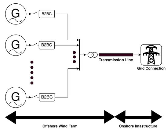
Figure 1.
Traditional Interconnection.
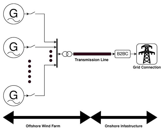
Figure 2.
Direct Interconnection.
In the case of the traditional interconnection, each generator is effectively separated from the local wind farm bus by the B2BC in the wind tower. This facilitates separation of the generator, and transients caused by wind gusts for example, from the local farm bus, and the individual B2BC provides a means of dealing with transient conditions on the generator side [25]. With DIT, as multiple generators are directly interconnected to the same bus, any gust generated transient condition experienced initially by a leading-turbine-to-wind will affect the interconnected system of generators.
This paper studies the effects of wind gusts by simulating a directly interconnected wind farm and introducing a wind gust to a leading turbine. Gusts of varying types, magnitudes and transient times are applied to a leading turbine and overall system responses are investigated as described in detail in the simulation methodology section. Gust tolerance levels are measured and discussed with comparison to real-world coastal wind data.
2. Simulation Methodology
Gusts modelled in this study are created through the use of IEC standardised descriptions of gusts available in IEC 61400-3-1:2019 [26]. This offshore wind turbine standard in section 6.4.3.1 directly refers back to IEC 61400-1:2019 [27], an onshore wind turbine standard that describes the mean wind speed based wind gust profiles. In this standard, five extreme wind conditions are proposed: Extreme Operating Gusts (EOG), Extreme Direction Change (EDC), Extreme Coherent Gusts (ECG), Extreme Coherent Gusts with direction change (ECD) and Extreme Wind Shear (EWS). This study focuses on EOG and ECG. ECGs are considered as the increase in wind speed is sustained once the maximum gust speed is reached. This gust profile is useful for identifying any saturation limits of the system whereas the Mexican hat shape of EOGs present the greatest rate of change during the gust and therefore challenge the system due to the maximum rate of change of pitch angle. This worst-case analysis approach does not consider direction change of the wind, as the greatest amount of energy and therefore the most challenging input for the directly interconnected bus, occurs when the wind is directly incident on the turbine blades [28]. All gusts are applied with the hub facing directly into the wind with no yaw control considered. Future work may include an analysis of the other conditions. EOG and ECG profiles are generated using Equations (1) and (2).
As defined in IEC 61400-1, is the hub height magnitude defined by extreme wind speed recurrences for a particular site along with other physical factors such as rotor diameter. This factor is varied along with the period T to peak gust speed and settling time. is the average wind speed upon which the wind gust is superimposed.
In Equation (2), is the average wind speed, is the magnitude of the coherent gust and T represents the rise time of the gust. Once the gust is complete the wind speed remains at this new value of . A sample of each gust type with the same rise time of five seconds is shown in Figure 3.
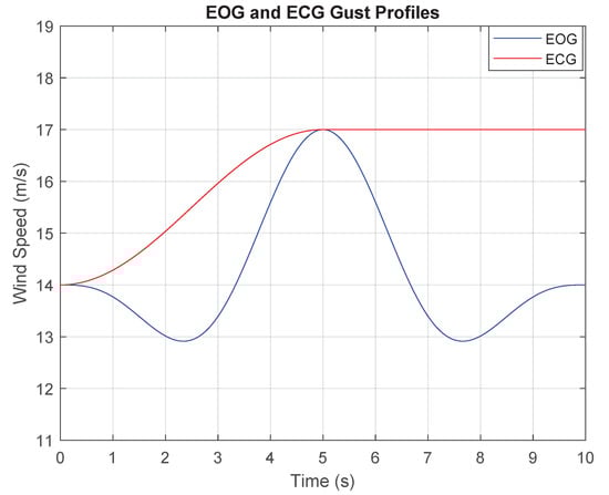
Figure 3.
EOG and ECG profiles with rise times of 5 s.
The characteristic time for ECGs/EDCs stated in IEC 61400-1:2019 6.3.3.6 is 10 s [27]. This represents a rise time of 10 s between the base wind speed and the maximum wind speed value. However, in the case of EOGs in section 6.3.3.3, the characteristic time is 10.5 s. This time represents the length of the entire gust. Therefore the corresponding rise time would be 5.25 s. For this study, we round down this rise time to 5 s and consider rise times of 3 s, 5 s and 10 s to investigate these gusts on a like for like basis. These values are representative of the gust profiles as described in the standard, but also push beyond the values to investigate system limits.
Each turbine utilises a Permanent Magnet Synchronous Generator (PMSG) with a rated power of 800 kVA and is based on a real-world turbine characterisation [29]. The rated speed was selected at 14 m/s. The simulation begins with all wind turbines interconnected as per the direct interconnection algorithm described in [13]. Turbine 5 is selected as the pilot generator responsible for the maintenance of the frequency and voltage of the interconnected bus. This turbine in the real world would be selected as a turbine towards the centre of the wind park, thus minimising the risk of this turbine being the first to experience a wind disturbance. Each turbine has its own local dump load for spin up and disconnection from the main bus. A simulation diagram is shown in Figure 4. Disconnection could be required for dispatching down, in line with Transmission System Operator (TSO) instructions [30] or during times when the wind speed is outside of cut in and cut out speeds.
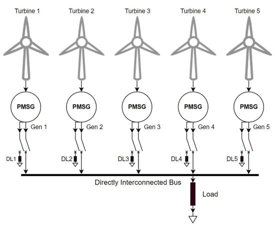
Figure 4.
Simulation Diagram Showing the five turbines with their respective dump loads, the directly interconnected bus and the main load for the farm.
2.1. Simulation Model
2.1.1. Permanent Magnet Synchronous Generator model
As defined in [31] the PMSG model behaviour is described in Rotor Reference Frame (RRF) as follows:
where R is the resistance of the stator windings, p is the number of pole pairs, is electrical torque, and are the axis inductances, is angular velocity of the rotor, is amplitude of induced flux, and are voltages and and are currents. Equations (3) and (4) represent the ouput currents and volatges in frame and Equation (5) calculates electromagnetic torque.
and represent the relation between the phase inductance and the rotor position due to the saliency of the rotor. For a round rotor, there is no variation in the phase inductance therefore .
2.1.2. Wind Turbine Model
The Wind turbine is modelled using the Matlab Simulink wind turbine model with a nominal mechanical output power of 800 kW and a base wind speed of 14 m/s. The output of this block is applied to the generator shaft in per unit of generator ratings. We assume a direct drive system where mechanical efficiency () is 1. This wind turbine characteristic can be seen in Figure 5.
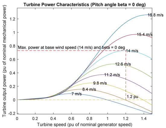
Figure 5.
Wind Turbine Model Power Characteristic Curve.
A PID blade pitch angle controller is used with a rate of change limitation of eight degrees per second. This is to account for the fact that pitch angle cannot be varied instantaneously. This rate of change limitation value can be found in the NREL 5 MW reference wind turbine report [32]. A full control and simulation diagram can be found for both the pilot generator in Figure 6 and for non-pilot generators in Figure 7. For the pilot generator, the control system utilises a frequency setpoint and feedback loop to maintain the farm bus frequency. This pilot generator is set to a chosen power level and excluded from the farm power control loop. Non-pilot generators use a power reference and feedback loop to vary their active power contribution to the bus. The setpoint for these turbines is determined by a farm power level supervisor which takes the current farm power level and set point and distributes individual power levels to the turbines. For further information on the direct interconnection algorithm, see [13,24,29].
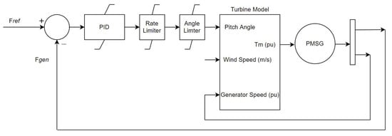
Figure 6.
Control and Simulation Diagram for the Pilot Generator.
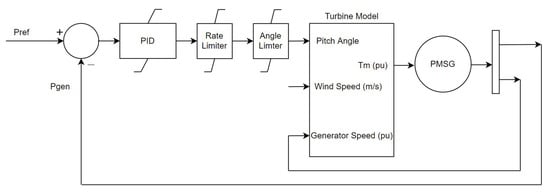
Figure 7.
Control and Simulation Diagram for the Non-Pilot Generators.
2.2. Simulation Parameters
The simulation parameters utilised in this study are provided by the company JSPM, a subsidiary of the Areva group, and represent a real-world PMSG turbine [33]. These values are applied to each PMSG model in the simulation. This characterisation is employed to provide a consistent simulation analysis approach for DIT. These parameters displayed in Table 1 as used by Pican and Ebrahimi Salari [24,29], provide a basis for comparison of DIT in varying configurations and conditions. The farm size selection of 5 turbines is presented as the base number of turbines which would realistically be deployed in the field. Larger farms could be made up of a single directly interconnected bus or multiple strings of directly interconnected buses, each consisting of varying numbers of turbines due to transmission, resource availability or geographical constraints [34,35,36]. A larger number of interconnected generators, similar to the traditional AC power gird, will facilitate better sharing of disturbances and simplify the frequency and power response of the system.

Table 1.
Simulation Parameters [33].
2.3. Gust Factor and Variation Limits
Gust Factor is a representation of the peak average second wind speed as a fraction of the T seconds moving average wind speed [37]. This is shown in Equation (6), where is the maximum second moving average wind speed in a T-second averaging period and is the T-second average wind speed. Typical values for are 1–10 s with common values for T are 10 min to 1 h [37]. The gust factors of all test gusts applied are calculated and analysed.
The tolerance threshold for both measured parameters of the simulation is selected as 5% (). This threshold is selected to closely follow current grid connection codes on the farm side of the power converter [38]. This paper shows the differing gird requirements that the power conversion system of wind turbines are required to comply with. By limiting variation of frequency and active power to 5%, the power conversion system will be able to ensure grid interconnection compliance [30].
3. Results
3.1. Baseline System Response
The baseline system response is generated applying the reference wind gust to the leading turbine while all pitch controllers on turbines 1–5 are disabled. This shows the reaction of the interconnected system of wind turbines in the absence of controllers assisting in dealing with gust disturbances. As shown in Figure 8 without any pitch control the system behaves similar to a single synchronous machine causing the collective bus frequency to increase while active power is inserted at the lead turbine. This relatively small disturbance causes both the bus active power and bus frequency responses to vary outside the 5% () tolerance threshold.
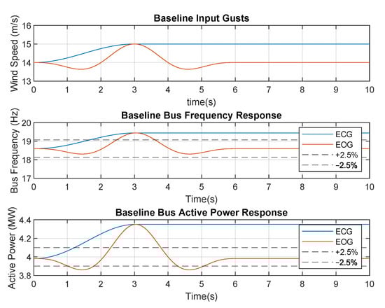
Figure 8.
Baseline system test for both ECG and EOG. s max = 15 m/s.
3.2. Extreme Coherent Gust Responses
The following section displays simulations results for Extreme Coherent Gusts (ECG) as described in the IEC Standard [27]. The test gust is applied to generator one with the system at a steady state at time zero. All generators are synchronised and interconnected to the main bus before time zero and have reached a steady state. Extreme coherent gust simulations are preformed at values of 3 s, 5 s and 10 s respectively. Example test gusts for s are displayed in Figure 9.
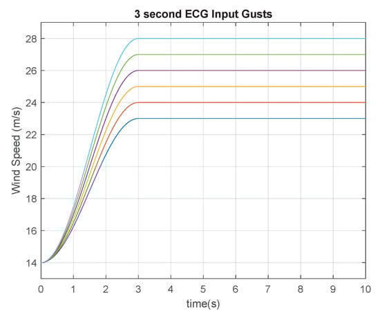
Figure 9.
3 s ECG test gusts applied.
For each rise time max is varied from 15 m/s to 30 m/s in 1 m/s increments. The corresponding gust factors of these gusts can be calculated by Formula (6), where is the maximum second moving average wind speed in a T-second averaging period and is the T-second average wind speed [37]. The gust factors for the input ECG test gusts applied are displayed in Table 2 assuming a ten minute moving average base wind speed = 14 m/s and s.
Table 2.
ECG Input Gust Factors.
Figure 10 displays the frequency responses of each gust measured at the offshore bus. As can be clearly seen the 28 m/s gust response exceeds the limit of 5% () variation. This is due to the rate of change limitation of pitch angle variation of turbines. With an 8 degree per second maximum rate the pitch control is not capable of maintaining the 5% maximum variation. However, it can be seen that the system can damp the variation and return to steady state in all of the input gust cases. The 27 m/s gust also approaches the negative 2.5% limit but does not exceed it and therefore can be taken to be the maximum boundary limit with regard to our frequency response criteria.
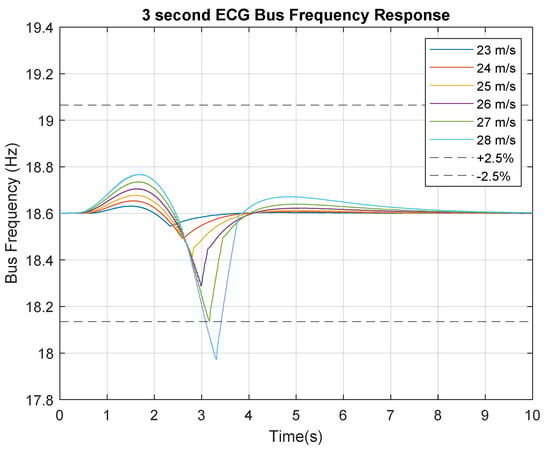
Figure 10.
System frequency response to 3 s ECG gusts.
As can be seen in Figure 10 and Figure 11, the active power and the frequency response are directly linked. As the 28 m/s ECG is rejected due to the frequency response criteria it can already be discounted. The 26 m/s, 27m/s and 28 m/s responses all fall outside the negative boundary leaving the 25 m/s as the maximum boundary within the limit with regard to the active power criteria. It can therefore be said that for the system modelled any ECG with of 3 s and magnitude up to and including 25 m/s can be tolerated.
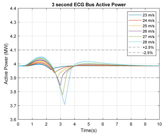
Figure 11.
Bus active power response to 3 s ECG gusts.
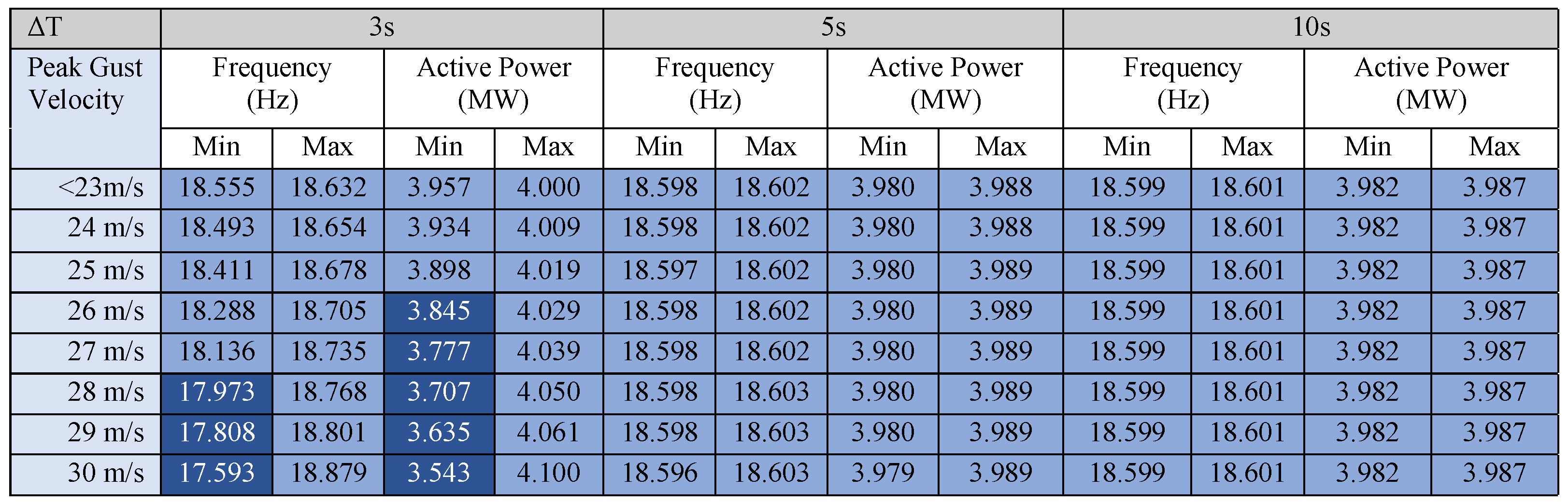
The remaining simulations for ECGs with s and s all show performance within the 5% tolerance level. The 8 degrees/s of pitch angle control is capable of damping response without becoming saturated. The results of all the simulations are tabulated in Table 3. The light blue segments denote the respective criteria are satisfied while dark blue denotes that one or both of the threshold levels have been exceeded. Considering the 5 s and 10 s rise time simulations, it can be observed that ECGs up to 30 m/s can be tolerated by the system. The maximum gust factors for these events of 1.64 through 2.14 are well beyond the gust factors measures at the coastal wind site in Frøya [37]. The 3 s ECG is within limits up to and including a max of 25 m/s. With a gust factor of 1.79 from Table 2, this 25 m/s gust is well above the measured gust factors at this site with a mode value of 1.20.
Table 3.
This table displays the results of all ECG simulations completed. Light Blue demonstrates the respective responses remain within the boundary limitations with dark blue showing the criteria has not been met. The minimum and maximum values of both frequency and active power reached during each gust are displayed.
3.3. Extreme Operating Gust Responses
This section outlines the Extreme Operating Gust responses for values of 3 s, 5 s and 10 s. The same initial conditions of synchronisation and steady state are utilised with the gust being applied to turbine 1 at time t = 0. The max values are incremented by 1 m/s from 15 m/s to 30 m/s. Example 3 s EOG input gusts can be seen in Figure 12.
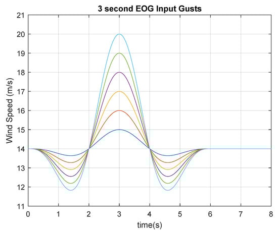
Figure 12.
3 s EOG test gusts applied.
The corresponding gust factors for the 3 s, 5 s and 10 s rise time EOGs are calculated by integrating (1) with limits of ±0.5 s of the peak gust time giving the sliding window of s and are displayed in Table 4. The 10 min moving average wind speed m/s.
Table 4.
EOG Input Gust Factors.
Considering Figure 13, it can clearly be seen that the wind farm struggles to maintain electrical frequency through EOGs, when compared with ECGs of the same magnitude displayed in the previous section. This is to be expected as now the leading turbine first experiences a dip in wind speed prior to the sharp rise to max. It can be observed that EOGs with magnitudes greater than 18 m/s lead to a violation of the 5% pk-pk limitation on bus frequency. The initial negative dip in wind speed preceding the rise causes a greater which saturates the 8 degree per second rate of change limitation on the pitch controller.
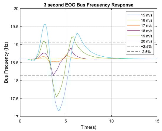
Figure 13.
System frequency response to 3 s EOG gusts.
Figure 14 displays the active power variation on the main bus through the event. It can be seen that the 18 m/s gust displayed in purple, while within tolerance levels for frequency variation, fails to remain within 5% limitation on active power. However, as the active power only exceeds this limitation by 100 kW, it is possible that it could be considered tolerable in some electrical power conversion systems, particularly those which incorporate storage. This simulation assumes that all wind turbines remain connected to the bus throughout the transience however in the higher cases of max, it is likely that the turbine would be forced to disconnect from the main bus. This case however is outside the scope of this study and may be explored in future work.
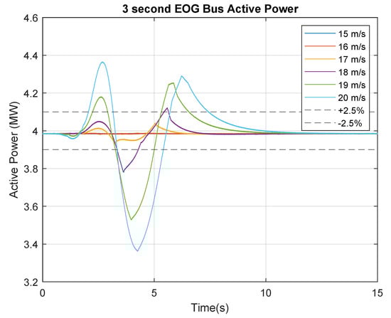
Figure 14.
Bus active power response to 3 s EOG gusts.
The system frequency responses as shown in Figure 15 display a similar trend to that of the three second EOG tests. We can see however that the 19 m/s is within tolerable limits with the 20 m/s forming the boundary condition with regard to system frequency.
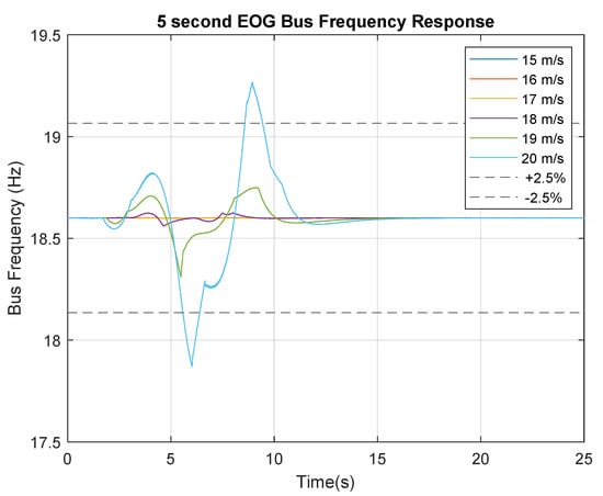
Figure 15.
EOG Bus Frequency Responses s.
Figure 16 displays the bus active power variation for the 5 s EOG tests. It can be observed that the 19 m/s EOG trace shown in green falls outside the negative 2.5% variation limit for a short period of time. For the purposes of this study, this will be declared outside the tolerance range.
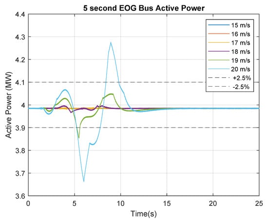
Figure 16.
EOG Bus Active Power Responses s.
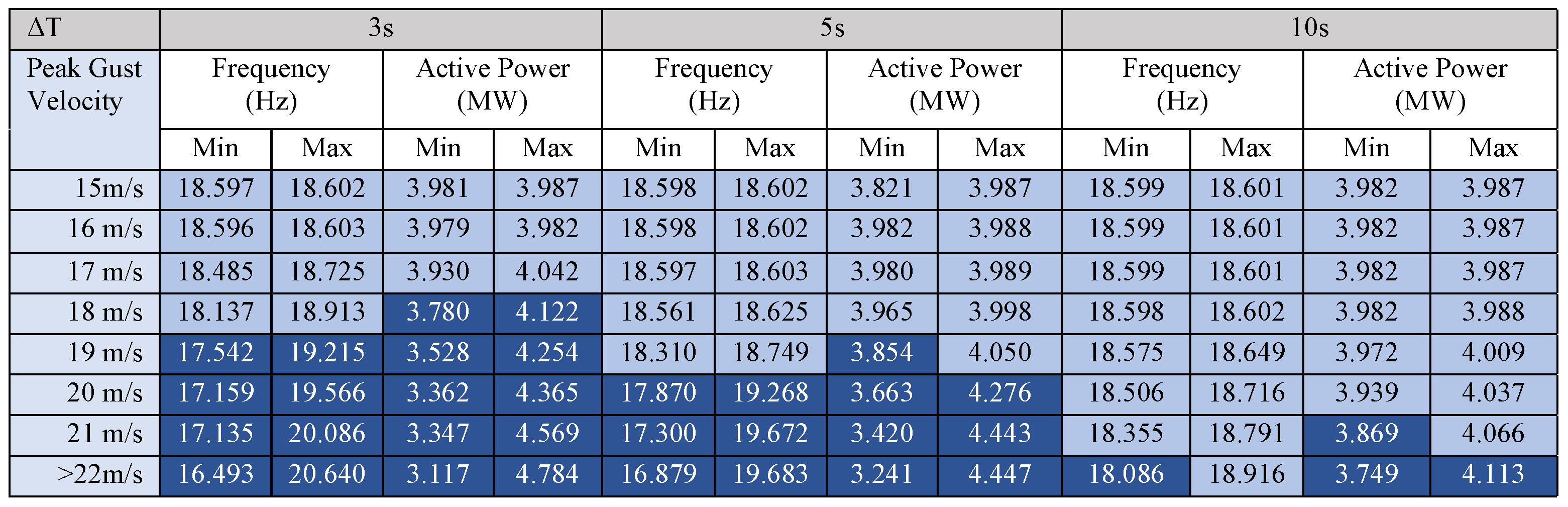
All test runs are displayed in Table 5. The light blue denotes the output remains within the respective boundary condition with dark blue showing that one or both of the boundaries have been exceeded.
Table 5.
This table displays the results of all EOG simulations completed. Light Blue demonstrates the respective responses remain within the boundary limitations with dark blue showing the criteria has not been met.
Analysing Table 5, it can be observed that the EOG gusts present a much greater challenge to the DIT bus parameters than ECGs. The 10 s rise time EOGs are the most effectively controlled which is to be expected as they have the lowest rate of change of max. The gust factors for these gusts are higher than the gust factors for shorter rise time gusts of the same magnitude. This is due to the wind speed cresting the maximum point for a greater time on either side of the maximum, therefore increasing the 1 s sliding average value. For a rise time of 10 s, the maximum gust factor which was successfully controlled by blade pitch angle control is 1.424. This gust factor is significantly below the 10 s for ECGs of 2.14 and above. Comparing this to the findings of Bardal et al., it can be observed that gust factors of 1.4 and above at the 100 m hub height are very rare [37]. As the average hub heights of modern offshore turbines are greater than 100 m, the 100 m data is the most relevant to this study.
If we consider the 3 and 5 s EOG data the corresponding boundary gust factors of 1.189 and 1.273 are within the range of values experienced offshore [37], however, the majority of gusts in the study fall below these values. This study also includes gust factors of gusts which may have occurred during times when the average wind speed may have been above the typical cut out speed of the turbine of 25 m/s and therefore the farm would not have been operating [39]. Gusts of this nature that do occur during the operation of a DIT wind farm would require further mitigation techniques outside of pitch angle control to maintain the 2.5% variation parameter studied.
4. Discussions & Conclusions
Extreme Operating and Coherent wind gust responses for directly interconnected systems have been investigated and discussed. It has been shown that through the use of pitch control on individual turbines the majority of wind gusts can be tolerated and the boundaries of this tolerance have been identified. The respective gust factors for these gust events have been calculated and compared to real coastal wind data [37]. These boundaries as presented in Table 3 and Table 5 form the basis for further study on DITs interconnection to the grid. Power converter design and location can be investigated to further improve the gust tolerance of DIT systems. Additional analysis of large wind data sets will provide estimates of the frequency of gusts with gust factors greater than the tolerance levels described, facilitating comparison of DIT and traditionally interconnected wind systems in terms of capacity factor, capital expenditure (CapEx) and operational expenditure (OpEx).
Extreme operating gusts pose a greater challenge when compared to the extreme coherent gust conditions due to the higher rate of change in wind speed occurring throughout the gust. This study has not used B2BC which ordinarily provide a means on an individual turbine by turbine basis, of dealing with variations on the wind side while maintaining power on the grid side within specified limits of frequency and voltage. In the proposed DIT topology it is still intended to use B2BCs for a number of turbines as shown in Figure 2. Employing the farm level B2BC control and the pitch control as analysed in this paper will facilitate a greater tolerance range of gusts for DIT systems and will be the subject of future work. It is possible that with wind prediction methods such as LiDAR and more sophisticated machine learning-based control systems, that the boundaries could be further improved thereby reducing the load on the pitch control system and the power conversion systems down steam of the interconnected bus.
In conclusion, the Direct Interconnection Technique has been shown to be capable of tolerating wind gust conditions. The boundary of tolerance has been established and methods for further improvement have been proposed.
Author Contributions
C.W.O. carried out the reported research work, writing the paper and revisions. M.E.S. and D.J.T. supervised the research work, revisions and editing. The content of this paper is discussed by the authors and they all contributed to the final article. All authors have read and agreed to the published version of the manuscript.
Funding
This publication has emanated from research supported by the Science Foundation Ireland under the MaREI Centre research programme (Grant No. 12/RC/2302, and 14/SP/2740) and LERO Science Foundation Ireland grant 13/RC/2094. It is also co-funded under the European Regional Development Fund through the Southern and Eastern Regional Operational Programme to MaREI (www.marei.ie (accessed on 20 December 2021)) and Lero (www.lero.ie (accessed on 20 December 2021)) centres.
Institutional Review Board Statement
Not applicable.
Informed Consent Statement
Not applicable.
Data Availability Statement
Data Available on request.
Conflicts of Interest
The authors declare that the publication of this article has no conflict of interest.
References
- Gallagher, S.; Tiron, R.; Whelan, E.; Gleeson, E.; Dias, F.; McGrath, R. The nearshore wind and wave energy potential of Ireland: A high resolution assessment of availability and accessibility. Renew. Energy 2016, 88, 494–516. [Google Scholar] [CrossRef]
- Jung, C.; Schindler, D.; Buchholz, A.; Laible, J. Global Gust Climate Evaluation and Its Influence on Wind Turbines. Energies 2017, 10, 1474. [Google Scholar] [CrossRef] [Green Version]
- Department of the Environment, Climate and Communications. Ireland’s National Energy and Climate Plan 2021–2030; Government of Ireland: Dublin, Ireland, 2021. Available online: https://www.gov.ie/en/publication/0015c-irelands-national-energy-climate-plan-2021-2030/ (accessed on 20 December 2021).
- SEAI. Wind Energy Roadmap 2011–2050. 2011. Available online: https://www.seai.ie/publications/Wind_Energy_Roadmap_2011-2050.pdf (accessed on 20 December 2021).
- Harper, M.; Anderson, B.; James, P.A.B.; Bahaj, A.S. Onshore wind and the likelihood of planning acceptance: Learning from a Great Britain context. Energy Policy 2019, 128, 954–966. [Google Scholar] [CrossRef]
- Brand, A.J.; Peinke, J.; Mann, J. Turbulence and wind turbines. J. Phys. Conf. Ser. 2011, 318, 072005. [Google Scholar] [CrossRef]
- Moriarty, P.J.; Holley, W.E.; Butterfield, S. Effect of Turbulence Variation on Extreme Loads Prediction for Wind Turbines. J. Sol. Energy Eng. 2002, 124, 387–395. [Google Scholar] [CrossRef]
- Ebrahimi, A.; Sekandari, M. Transient response of the flexible blade of horizontal-axis wind turbines in wind gusts and rapid yaw changes. Energy 2018, 145, 261–275. [Google Scholar] [CrossRef]
- Onol, A.O.; Yesilyurt, S. Effects of wind gusts on a vertical axis wind turbine with high solidity. J. Wind. Eng. Ind. Aerodyn. 2017, 162, 1–11. [Google Scholar] [CrossRef]
- Cheng, P.W.; Bierbooms, W.A.A.M. Distribution of extreme gust loads of wind turbines. J. Wind. Eng. Ind. Aerodyn. 2001, 89, 309–324. [Google Scholar] [CrossRef]
- Zhou, K.; Cherukuru, N.; Sun, X.; Calhoun, R. Wind Gust Detection and Impact Prediction for Wind Turbines. Remote Sens. 2018, 10, 514. [Google Scholar] [CrossRef] [Green Version]
- Dhiman, H.S.; Deb, D.; Muresan, V.; Balas, V.E. Wake Management in Wind Farms: An Adaptive Control Approach. Energies 2019, 12, 1247. [Google Scholar] [CrossRef] [Green Version]
- Pican, E.; Omerdic, E.; Toal, D.; Leahy, M. Direct interconnection of offshore electricity generators. Fuel Energy Abstr. 2011, 36, 1543–1553. [Google Scholar] [CrossRef] [Green Version]
- Meng, Y.; Yan, S.; Wu, K.; Ning, L.; Li, X.; Wang, X.; Wang, X. Comparative economic analysis of low frequency AC transmission system for the integration of large offshore wind farms. Renew. Energy 2021, 179, 1955–1968. [Google Scholar] [CrossRef]
- Rahman, S.; Khan, I.; Alkhammash, H.I.; Nadeem, M.F. A Comparison Review on Transmission Mode for Onshore Integration of Offshore Wind Farms: HVDC or HVAC. Electronics 2021, 10, 1489. [Google Scholar] [CrossRef]
- Spinato, F.; Tavner, P.J.; Bussel, G.J.W.v.; Koutoulakos, E. Reliability of wind turbine subassemblies. IET Renew. Power Gener. 2009, 3, 387–401. [Google Scholar] [CrossRef] [Green Version]
- Zhao, Y.; Li, D.; Dong, A.; Kang, D.; Lv, Q.; Shang, L. Fault Prediction and Diagnosis of Wind Turbine Generators Using SCADA Data. Energies 2017, 10, 1210. [Google Scholar] [CrossRef] [Green Version]
- Ren, Z.; Verma, A.S.; Li, Y.; Teuwen, J.J.E.; Jiang, Z. Offshore wind turbine operations and maintenance: A state-of-the-art review. Renew. Sustain. Energy Rev. 2021, 144, 110886. [Google Scholar] [CrossRef]
- Hossain, M.L.; Abu-Siada, A.; Muyeen, S.M. Methods for Advanced Wind Turbine Condition Monitoring and Early Diagnosis: A Literature Review. Energies 2018, 11, 1309. [Google Scholar] [CrossRef] [Green Version]
- Lu, B.; Sharma, S.K. A Literature Review of IGBT Fault Diagnostic and Protection Methods for Power Inverters. IEEE Trans. Ind. Appl. 2009, 45, 1770–1777. [Google Scholar] [CrossRef]
- Qiao, W.; Lu, D. A Survey on Wind Turbine Condition Monitoring and Fault Diagnosis—Part I: Components and Subsystems. IEEE Trans. Ind. Electron. 2015, 62, 6536–6545. [Google Scholar] [CrossRef]
- Johnston, B.; Foley, A.; Doran, J.; Littler, T. Levelised cost of energy, A challenge for offshore wind. Renew. Energy 2020, 160, 876–885. [Google Scholar] [CrossRef]
- Su, C.; Yang, Y.; Wang, X.; Hu, Z. Failures analysis of wind turbines: Case study of a Chinese wind farm. In Proceedings of the 2016 Prognostics and System Health Management Conference (PHM-Chengdu), Chengdu, China, 19–21 October 2016; pp. 1–6. [Google Scholar] [CrossRef]
- Ebrahimi Salari, M.; Coleman, J.; Toal, D. Power Control of Direct Interconnection Technique for Airborne Wind Energy Systems. Energies 2018, 11, 3134. [Google Scholar] [CrossRef] [Green Version]
- Li, S.; Haskew, T.A.; Swatloski, R.P.; Gathings, W. Optimal and Direct-Current Vector Control of Direct-Driven PMSG Wind Turbines. IEEE Trans. Power Electron. 2012, 27, 2325–2337. [Google Scholar] [CrossRef]
- IEC. EN IEC 61400-3-1:2019 Part 3-1: Design Requirements for Fixed Offshore Wind Turbines; International Electrotechnical Commission: Geneva, Switzerland, 2019. [Google Scholar]
- IEC. EN IEC 61400-1:2019 Wind Energy Generation Systems—Part 1: Design Requirements; International Electrotechnical Commission: Geneva, Switzerland, 2019. [Google Scholar]
- Yang, J.; Fang, L.; Song, D.; Su, M.; Yang, X.; Huang, L.; Joo, Y.H. Review of control strategy of large horizontal-axis wind turbines yaw system. Wind Energy 2021, 24, 97–115. [Google Scholar] [CrossRef]
- Pican, E.; Omerdic, E.; Toal, D.; Leahy, M. Analysis of parallel connected synchronous generators in a novel offshore wind farm model. Energy 2011, 36, 6387–6397. [Google Scholar] [CrossRef]
- Eirgrid. General Conditions of Connection and Transmission Use of System; Eirgrid Group: Dublin, Ireland, 2013. [Google Scholar]
- Grenier, D.; Dessaint, L.A.; Akhrif, O.; Bonnassieux, Y.; Le Pioufle, B. Experimental nonlinear torque control of a permanent-magnet synchronous motor using saliency. IEEE Trans. Ind. Electron. 1997, 44, 680–687. [Google Scholar] [CrossRef]
- Jonkman, J.; Butterfield, S.; Musial, W.; Scott, G. Definition of a 5-MW Reference Wind Turbine for Offshore System Development; Technical Report NREL/TP-500-38060, 947422; National Renewable Energy Laboratory: Golden, CO, USA, 2009. [CrossRef] [Green Version]
- Leroy, F. JSPM Filial of AREVA NP; Areva S.A.: Courbevoie, France, 2011. [Google Scholar]
- Bahirat, H.J.; Mork, B.A.; Høidalen, H.K. Comparison of wind farm topologies for offshore applications. In Proceedings of the 2012 IEEE Power and Energy Society General Meeting, San Diego, CA, USA, 22–26 July 2012; pp. 1–8. [Google Scholar] [CrossRef]
- Sedighi, M.; Moradzadeh, M.; Kukrer, O.; Fahrioglu, M. Simultaneous optimization of electrical interconnection configuration and cable sizing in offshore wind farms. J. Mod. Power Syst. Clean Energy 2018, 6, 749–762. [Google Scholar] [CrossRef] [Green Version]
- Wu, Y.; Zhang, S.; Wang, R.; Wang, Y.; Feng, X. A design methodology for wind farm layout considering cable routing and economic benefit based on genetic algorithm and GeoSteiner. Renew. Energy 2020, 146, 687–698. [Google Scholar] [CrossRef]
- Bardal, L.M.; Sætran, L.R. Wind Gust Factors in a Coastal Wind Climate. Energy Procedia 2016, 94, 417–424. [Google Scholar] [CrossRef] [Green Version]
- Singh, B.; Singh, S.N. Wind Power Interconnection into the Power System: A Review of Grid Code Requirements. Electr. J. 2009, 22, 54–63. [Google Scholar] [CrossRef]
- Dupont, E.; Koppelaar, R.; Jeanmart, H. Global available wind energy with physical and energy return on investment constraints. Appl. Energy 2017, 209, 322–338. [Google Scholar] [CrossRef]
Publisher’s Note: MDPI stays neutral with regard to jurisdictional claims in published maps and institutional affiliations. |
© 2021 by the authors. Licensee MDPI, Basel, Switzerland. This article is an open access article distributed under the terms and conditions of the Creative Commons Attribution (CC BY) license (https://creativecommons.org/licenses/by/4.0/).