Abstract
This paper investigates the possibility of converting vibrations to electricity. A numerical and an experimental study of a magnetic levitation harvester are proposed. The system can be highly efficient when the electrical parameters are correctly tuned. Mechanical and electrical interaction of the harvester is described by an electromechanical coupling. Fixed value, linear and nonlinear electromechanical coupling models are presented and compared. It has been shown that the nonlinear electromechanical coupling model is more suitable for higher oscillations of the magnet. The obtained results show that nonlinear resonance and recovered energy can be controlled by the simple configuration of the magnet coil position. The recovered energy from the top branch is significantly higher, but this solution is much harder to obtain.
1. Introduction
1.1. Energy Harvesting
With an increase in the demand for electricity, there are increased requirements for alternative energy sources. One of the options for meeting this demand is to harvest energy from ambient vibrations. The literature referencing the systems that convert mechanical vibrations to usable electrical energy is extremely wide. This process is usually known as energy harvesting (EH) or energy scavenging (ES). Increasing solutions developed by scientists lead to frequent use of harvester devices in practice; for example, information and communication technologies [1], the Internet of Things [2,3], wireless technology [4] and powered electronic devices [5,6]).
Vibration energy harvesters (VEHs) require a transduction mechanism that couples the mechanical system with the electrical part. The conversion techniques are usually based on electromagnetic, piezoelectric or electrostatic effects. However, as reported in [7], two methods are dominant in vibration harvesters: piezoelectric and electromagnetic. VEHs usually differ in architecture, size, excitation method, and output performance. They are preferable in some engineering applications for their smaller internal impedance and larger current output when compared to other ones [8]. One of the popular harvesters belonging to an electromagnetic group is a cylindrical magnet that oscillates in a coil. The magnet motion can be achieved through mechanical or magnetic springs, or can be freely moving (magnetic levitation harvester) [9,10]. Saha [11] et al. showed magnetic levitation generator for harvesting energy from human motion. The harvester was placed inside a rucksack and the power was measured during walking and running. The prototype harvester generated about 2.5 mW during walking and slow running. Rome et al. [12] analyzed a similar harvester and an electromagnetic suspended load back was applied for vertical movement during walking. Large-scale electromagnetic vibration harvesters are considered a viable source of renewable energy. For example, Zuo et al. [13] showed that tall buildings can be a source of kilowatts of power due to wind excitation. Different electromagnetic harvesters have also been applied in vehicles [14], railway systems [15], seismic events [16] and on the ocean floor [17]. Rhinefrank et al. [18] proposed a buoy-type ocean wave magnetic energy harvester, where a permanent magnet generator was used to harvest the vertical components of ocean waves. Masoumi and Wang [19] have investigated magnetic levitation energy harvester (called repulsive magnetic scavenger) dedicated to capable of harvesting ocean wave energy. Their prototype harvester reaches up to 42 V at the frequency of 9 Hz. A comprehensive review of the state-of-the-art on large-scale vibration energy harvesting is shown in [20].
1.2. Electromechanical Coupling
The amount of electricity recovered from an electromagnetic harvester depends not only on the strength of the magnetic field, but also on the velocity of the relative motion between the magnet and coil and the coil parameters (turns, resistance). A characteristic feature of energy harvesters is the electromechanical coupling (EC) coefficient. One of the most common methods of EC modeling is to treat it as a constant electrical damping value [21,22,23,24]. This approach indicates that the electromechanical coupling effect can be treated as a mechanical force opposing the relative motion due to Lenz’s law. Camarano [25] showed the analysis of a nonlinear energy harvester with hardening compliance and electromagnetic transduction under the assumption of negligible inductance and a constant EC coefficient. The author also proposed a method based on numerical continuation to find the optimum load for a harvester with fixed sinusoidal excitation. Mann [26] demonstrated a maglev harvester with a fixed EC coefficient. It has been shown that the nonlinearity of the harvester could improve the energy recovery bandwidth. Zhu and Zu [27] used a magnetic levitation harvester, similar to [26], with a changing magnetic field in the magnetoelectric composite material. As this paper shows, the EC coefficient is not constant but dependent on the location of the magnet in the coil. The same conclusions have been drawn in the paper of Lee et al. [28]. The authors showed that the interaction between the magnetic force and the induced voltage should be modeled as nonlinear damping in contrast to constant damping. This increases the recovered energy by 18%. Avila Bernal and Linares Garcia [29] calculated the electromagnetic damping force exerted by an induced current coil with semi−analytical solutions. Soares dos Santos et al. [30] proposed a fully analytical study for modeling levitation-based harvesters. The studies were based on an analytical determination of the magnetic field with a Lorenz force expression. The EC was a function of the induced current. However, not enough information regarding the solution of the coupled model was given.
Martin Saravia [31] presented two formulations of the EC. He suggested that the classical formulation in terms of the electromechanical damping coefficient leads to an inconsistent description because of neglecting the electrical circuit’s reactance and injecting the electromechanical coupling as a mechanical dissipative force. Kecik [32] proposed that the EC can be described as a nonlinear function of the levitating magnet position in the coil terminal. However, he assumed that the floating magnet oscillates in the coil’s center. These analyses were expanded in [33], where the electrical parameters were additionally optimized. Other nonlinear forms of the EC coefficient have been considered as sum of the EC coefficient of each coil turn [34,35]. Several measurement methods for the estimation of the EC coefficient are presented in [36]. The average deviations between different methods and simulations were about 5%. The authors estimated EC coefficients by calculation of electrical damping (neglecting the coil’s inductance) by finite element analysis (Ansys electromagnetics software) using the measured optimum load resistance, based on the linear variation of the current through the coil and using the voltage spectrum near to the main resonance.
One of the best review papers on major breakthroughs in the scope of electromagnetic levitation harvesters and critical discussion is [37]. The authors compared twenty-one different configurations, their geometric and constructive parameters, optimization methods and harvesting performances. Only in 15% of cases was very good agreement found between experimental and numerical analyses. This means that this problem is still important and has not been fully explored.
1.3. Motivation
The impetus for this research was to explore and evaluate how to describe the electromechanical coupling which characterizes the interaction between mechanical and electrical components. As shown in the literature analysis, most papers have not received sufficient attention on the electromechanical coupling. Usually small oscillations are assumed and the electromechanical coupling effect as the constant damping force is simplified.
This paper aims at shedding some light and suggestions on electromechanical coupling modelling. The originality of the paper is the proposals of new EC models and their comparison. Additionally, frequency response, bifurcation analysis and multistability analysis are shown. The motivation is the real application of the proposed harvester. This system is used as the tuned mass absorber in the autoparametric vibration absorber–harvester system [38].
2. Materials and Methods
2.1. Electromagnetic Harvester Design
Figure 1a shows photo of the nonlinear electromagnetic harvester proposed in this paper. It is mainly composed of two fixed magnets mounted in the plexiglass tube ends, a freely moving cylindrical magnet and an induction coil. A floating magnet is suspended through the magnetic repelling force. The design allows the levitating magnet to effectively oscillate in the coil. The harvester system is mounted in the shaker TIRA and connected to the data acquisition system. To reduce the mechanical friction between the tube and magnet, a Teflon surface and air holes are applied. The magnets are arranged with opposite polarities introducing hardening-type nonlinearity into the system. Moreover, this design causes the response of the system to be wider than a linear resonant system under harmonic excitation. The detailed description of the electromagnetic levitation harvester and identification of the magnetic suspension model in papers [32,39] are presented.
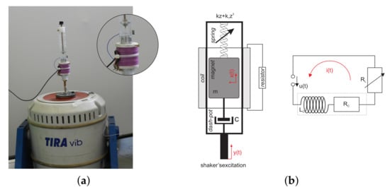
Figure 1.
Laboratory rig. (a) Prototype nonlinear magnetic harvester mounted on the shaker; (b) equivalent electromechanical system model of the harvester.
The magnetic levitation harvester can be simplified as a lumped-parameter model, as shown in Figure 1b. The magnet has a mass m, the magnetic force in this case is represented through a nonlinear Duffing spring with stiffness k and , and the linear term c represents the viscous damping and the magnet’s friction. The spring constants will depend on the size and strength of the fixed and moving magnets in the harvester. The generalized coordinates are represented by x, y and z (where z is the relative displacement = ). A harmonic displacement represented by y = Acos() is applied to the base, where A represents the shaker’s amplitude, is the excitation frequency and t is the time. The equations of motion for the system are:
The first equation represents the magnet motion and the second one the induced current. The electrical circuit consists of the coil with internal inductance L and internal and load resistances, respectively. The parameter g denotes the gravitational acceleration and is the induced current in the coil. is the electromechanical coupling coefficient (also called the electromagnetic coupling factor or transduction coefficient). This parameter describes the relationship between the mechanical and electrical domains of the electromagnetic energy harvester.
2.2. Electromechanical Coupling Determination
As shown in the introduction, there exists a considerable amount of literature regarding the determination of the electromechanical coupling as a constant value. In our prototype electromechanical harvester, the magnet oscillation can be large, including the magnet exit from the coil. In this study, the electromechanical coefficient was determined by giving a known value of the induced current from the dynamic test (Figure 2a).
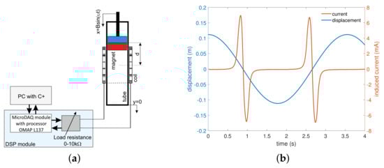
Figure 2.
Methodology of the dynamic magnet coil test. (a) Scheme of the dynamic test. (b) The two cycles of the dynamic test of the magnet moving through the coil with harmonic excitation; the exemplary measured current (red line) and the magnet’s displacement (blue line) were obtained for frequency = 1.7698 rad/s and amplitude B = 0.11 m.
The magnet was harmonically moved through the coil and the induced current and magnet displacement were measured. The exemplary results for induced current and the magnet displacement in Figure 2b are presented. The blue line denotes the magnet’s displacement, while the red line is the induced current. The test was performed for a fixed tube ( = 0), meaning that the relative displacement = . As we can see, the induced current is a strongly nonlinear function and a description of the electromechanical coupling by other functions seems to be justified.
2.3. Electromechanical Coupling Models
2.3.1. Constant EC Model
The electromechanical harvester is based on Faraday’s law of electromagnetic induction. When an electric part is moved through a magnetic field, then the electromotive force is induced. Generally, the induced voltage is the so-called electromotive force (emf) is proportional to the magnetic flux linkage change
where is the induced voltage and is magnetic flux. In the case of relative motion between the coil and the magnet in the z direction, Equation (3) for a coil with N turns can be modified to [36]
where can be interpreted as the average flux linkage per turn, B is the magnetic flux density and is the average length of a spiral coil. The parameter (Equation (5)) is the electromechanical coupling coefficient that depends on the coil geometry and the magnetic circuit and is expressed as
The standard approach for the description of the coupling between the electrical and mechanical domains is the constant value. This approach follows the fact that some research has treated the magnetic flux density as uniform over the coil volume and constant for the total range of motion (usually a small magnet’s oscillation). Note that the constant flux density assumption is not permissible for a large amplitude of the magnet’s motion. The high oscillation of the magnet in the coil causes strong variations in the magnetic flux density. Therefore, the coupling coefficient must be determined in a more accurate fashion.
2.3.2. Linear EC Model
In our harvester, the magnet can execute large amplitude oscillations (a few centimeters). Moreover, the magnet may move beyond the coil module. Therefore, the constant value of the electromechanical coupling will not describe the system behavior sufficiently. For these reasons the other coupling models have been proposed. First, a simple linear model of the electromechanical coupling function depending on the magnet’s position in the coil is proposed. This model is dedicated to the magnet oscillation in the vicinity of the coil center.
Using Kirchhoff’s law, the measured signals of induced current and the magnet velocity , the experimental electromechanical coupling function has been calculated and plotted in Figure 3.
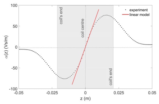
Figure 3.
The electromechanical coupling function (dots) and the proposed linear model (red line). This model is dedicated to magnet oscillation close to the coil’s center with magnet amplitudes not exceeding of 0.01 m.
Next, the linear model of the electromechanical linear coupling function (red line) was fitted to the experimental data (black points).
In Equation (6) the first derivative of the current is numerically calculated from the signal . The parameters L and R are the coil inductance and total coil resistance (), respectively. Note that the coil inductance is usually negligibly small (); therefore, this practically does not influence the value of . As reported in [39], in this harvester a coil inductance above 1 H begins to affect the dynamics.
Summarizing, the linear EC model can be mathematically written as
where the parameter means the slope of the red line. As we can see in Figure 3, the proposed EC model is convergent with the experimental data if the magnet oscillates in the coil center and the magnet’s amplitude does not exceed 0.01 m. For higher oscillation, a nonlinear model is proposed in the next section.
2.3.3. Nonlinear EC Model
For higher amplitudes of magnet vibrations (more than 0.01 m), the experimental electromechanical coupling curve has a complex shape (dots in Figure 4a). The EC function has the greatest value near the ends of the coil. Therefore, a polynomial approximation nonlinear model (red line in Figure 4a) is proposed. The polynomial model is easy to implement in numerical simulations.
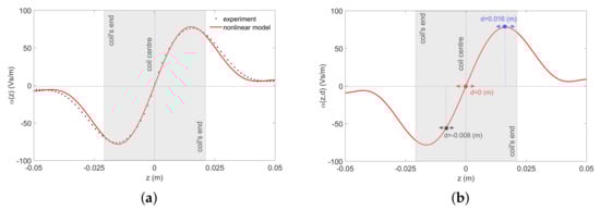
Figure 4.
Nonlinear electromechanical coupling model (a) compared with the experiment; (b) model including the magnet’s position in the coil. The black dots mean the experimental result, while the red line is the proposed nonlinear EC model. This model can be used for all ranges of the magnet motion and its different positions in a coil (parameter d). The highest value of parameter occurs close to the coil’s end.
A similar electromechanical coupling model has been proposed by Kecik et al. [32]. However, this model is modified by lowering the degree of the polynomial function and by introducing a new parameter d, which defines the position of the magnet in a coil (see Figure 2a). It is worth underlining that d influences the value of the electromechanical coupling. For example, close to d = 0 m (coil’s center), the electromechanical coupling can be treated as a linear function. As we can see, for other positions like d = 0.016 m (close to the coil’s end), this function becomes strongly nonlinear (Figure 4b). Therefore, we expect that this parameter can be important for the recovered energy.
The proposed mathematical nonlinear coupling model has the form
where the parameters and are determined by a least-squares curve-fitting technique.
3. Discussion of Electromechanical Coupling Models
3.1. Calculation Methods and Parameters
To explore the dynamics of the harvester, specific parameters were identified from the laboratory rig. The physical parameters of the laboratory system need to be quantified. Most of these are readily measurable or estimated: m = 0.1 kg, c = 0.054 Ns/m, k = 400 N/m, = 560 kN/m, L = 1.46 H, =1 k, = 0–20 k and g = 9.81 m/s. The logarithmic decrement technique was used to estimate the damping in the energy harvester. The magnetic stiffness parameters were estimated by fitting the magnetic force−displacement curve to a third-order polynomial. These coefficients were estimated by applying the least-squares method to fit the experimental data (see Figure 3 in paper [32]). The parameters k and represent the stiffness coefficients. This odd-power polynomial fit has been accepted and widely used in the literature [26].
The resonance frequency responses were obtained by the pseudo-arclength continuation technique, implemented by Doedel in the program AUTO [40] and verified in Matlab2020b. This software computes the stable and unstable periodic family solutions and the Floquet multipliers that determine stability. The solution is considered stable if the system returns to it after small disturbances. Moreover, the software allows precise computation of bifurcation points. The basins of attraction were calculated in the Matlab2020b and were verified in Dynamics software [41].
3.2. Comparing of Harvester with Different Electromechanical Coupling Models
In this section, the comparison of the harvester with different EC models is presented. Next, the best EC model is chosen and the harvester dynamics and energy recovery are analyzed in detail.
A comparison of the results of the magnet response and induced currents for the harvester with various electromechanical coupling models is presented in Figure 5a,b. The black line shows results from the harvester with the constant EC model, the blue line denotes results from the harvester with the linear EC model and the red line shows the harvester response with the nonlinear EC model. The green dots are the experimental shaker test results.
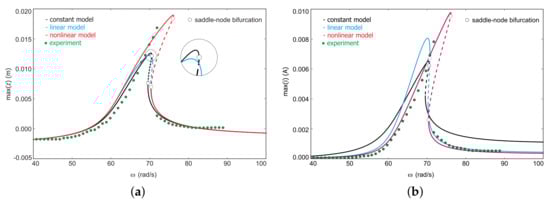
Figure 5.
Frequency–response curves of the maglev harvester with different electromechanical coupling models. (a) Relative magnet response. (b) Induced current. The black, blue and red lines show results from the model with constant, linear and nonlinear electromechanical coupling, respectively. The green dots are experimental results from the shaker tests. The solid line and the dashed line are the stable and unstable parts of the resonance branch, respectively. The circle means saddle-node bifurcation. All curves show nonlinear resonance with a hysteresis effect. The calculation were made for d = 0 m, A = 0.001 m and R = 10 k.
From both graphs, it can be seen that for all EC models the resonance occurs in the same place and the hardening effect is observed. The magnet’s oscillations of the harvester for all EC models are practically similar up to the frequency of 65 rad/s and above 77 rad/s. However, the recovered current differs in the whole range of frequencies. As reported in [32], the constant value of the EC can be accepted but must be very accurately estimated.
The maximal recovered energy for the harvester with the constant EC model is 0.42 W, with 0.64 W for the linear EC model and 0.98 W for the nonlinear EC model. The maximal recovered energy from the experiment was only 0.62 W. However, it should be noted that in the experimental tests it is very difficult to detect the total resonance curve, because the small distribution causes jumping of the magnet from the top to the bottom branch. The hardening effect characterizes two stable solutions and the amplitude jump caused by the saddle-node bifurcation (SNB) is most obvious for the system with the nonlinear EC model.
Comparing results of the harvester with different EC models we come to the conclusion that the nonlinear EC model most accurately describes the dynamics of the system. Therefore, in the next sections of this paper, we focus mainly on the analysis of the harvester with the nonlinear EC model.
4. Results
4.1. Frequency Response Curve
As we showed earlier, the electromechanical coupling is a strongly nonlinear function. The position of the oscillating magnet in the coil (parameter d) seems to be important. Therefore, in this section we evaluate the performance effectiveness of the harvester for three positions of the moving magnet in the coil.
The relationship between the location of an oscillating magnet in the coil and the response of a nonlinear harvester is complicated. Unlike in a linear system, the parameter d affects not only the amplitude of the response but also the shape of the entire frequency response. Figure 6a,b show the frequency response curves of the magnet and recovered current for different positions of the oscillating magnet. The red line presents the classical case, e.g., the magnet oscillates in the vicinity of center of the coil (d = 0 m). The blue line shows results for the oscillation of the magnet close to the coil’s end (d = 0.016 m) and the black line means the magnet position near to a quarter of the coil height (d = −0.008 m). The stable fixed points (branches) are marked by the solid line and dashed lines denote unstable ones. The unstable solution is caused by SNB point. This bifurcation is a typical mechanism for the creation/annihilation of fixed points. In this bifurcation point, an arbitrary small perturbation may lead to a sudden amplitude jump.
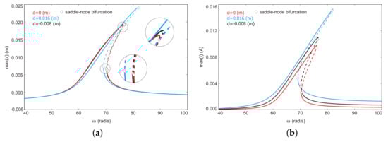
Figure 6.
Frequency–response curves of the maglev harvester. (a) Relative magnet response. (b) Induced current. The black, blue and red lines show results from the harvester with the nonlinear EC model for different magnet coil configurations. The solid line and the dashed line are stable and unstable solutions, respectively. The circle means saddle-node bifurcation. The calculations were made for A = 0.001 m. All response curves show nonlinear resonance with a foldover effect.
It can be seen that for d = 0.016 m, the hardening effect and the induced current are highest. The maximal recovered energy equals 2.4 W (for d = 0.016 m), 1.2 W (for d = −0.008 m) and 1 W (for d = 0 m). This clearly shows that the proper configuration of the magnet coil causes significantly higher recovered energy. Additionally, the multistability region can be wider (for d = 0 m: 70–76 rad/s, but for d = 0.016 m: 69–82 rad/s). This means that the recovered power during magnet oscillation close to the coil’s end is more effective. It results from the fact that the EC function reaches the highest value close to the coil’s end (see Figure 4). This leads to the real question of what happens with the harvester with the EC nonlinear function for other parameters and how the magnet coil configuration influences the multistability and basin of attraction.
4.2. Multistability Analysis
As previously discussed, the multistability depends on the EC function and it is therefore interesting to consider. For the basins of attraction in this paper, each simulation was performed for 1000 cycles to identify the final state of the harvester (the first 500 cycles were rejected as the transition time).
Figure 7a–d show the basins of attraction and coexistence of the two stable solutions under different positions of the oscillating magnet. These calculations were performed for frequency = 75 rad/s. Figure 7a presents the basin of attraction for d = 0 m, Figure 7b for d = −0.008 m, Figure 7c for d = 0.012 m, Figure 7d for d = 0.016 m, Figure 7e for d = 0.02 m and Figure 7f for d = 0.024 m.
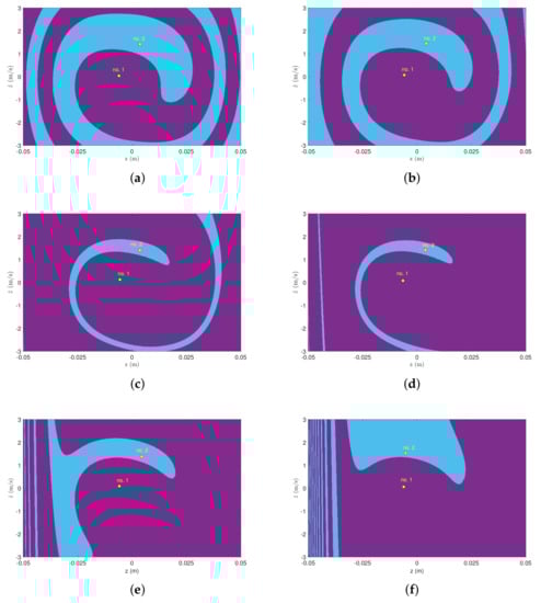
Figure 7.
Basins of attraction for the coexisting attractors for the frequency = 75 rad/s and resistance R = 10 k and with the increasing magnet position in the coil: (a) d = 0 m, (b) d = −0.008 m, (c) d = 0.012 m, (d) d = 0.016 m, (e) d = 0.02 m and (f) d = 0.024 m. The basins were constructed numerically. Here, the purple regions are the basins of attraction with attractor no. 1 corresponding to the bottom branch (low energy harvesting) and the blue region representing the basins of attraction with attractor no. 2 corresponding to the top branch (high energy harvesting). The probability of solution no. 2 decreases with a change in the magnet position from 42% (a), 36% (b), 10% (c), 6% (d), 20% (e) and 25% (f). The calculations were made for A = 0.001 m.
In these figures, the purple area represents the stable solution for the bottom branch (low energy output), while the blue area is for the top branch (high energy input). The attractors are marked by yellow dots and numbered 1 (for purple basins of attraction) and 2 (for blue basins of attraction). One can easily see that the basins represented by the blue color (high energy output) decrease if the position of the magnet moves away from the center of the coil. Then the low energy output (purple color) becomes dominant. For the magnet position d = 0 m, the probability of the high energy output equals 42 for d = −0.008 m the probability decreases to 36%, for d = 0.012 m the probability reduces to 10% and for d = 0.016 m the probability is the lowest 6%. Moreover, the probability of a high solution also increases just behind the coil (see Figure 7e,f).
This clearly indicates that the initial conditions for solutions no. 1 and no. 2 strongly depend on the position of the oscillating magnet in the coil. The probability of the solution was calculated based on the pixels of the basins of attraction (all basins were plotted in the same resolution). Note that the border between the two basins is cleared (not fractal). This could indicate the appearance of regular responses in the harvester.
To gain a better insight into the high energy output solutions, the probability versus parameter d was calculated (Figure 8). The higher probability of solution no. 2 occurs close to d = −0.025 m and in the vicinity of d = 0 m. Interestingly, this relationship is not symmetric. This is probably caused by the gravitational force and the nonlinearity of the system.
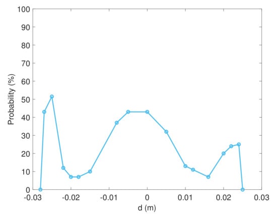
Figure 8.
Probability of high energy output versus the parameter d. The highest probability of solution no. 2 is located close to d = 0.025 m and close to the coil center. The calculations were made for A = 0.001 m.
Figure 9 and Figure 10 show the exemplary time histories of the magnet oscillation and the induced current close to the coil center (Figure 9a,b) and close to the coil’s end (Figure 10a,b). The purple color indicates the solution from the bottom branch, while the blue line shows the time response from the top branch. These solutions correspond to the attractors no. 1 and no. 2 from Figure 6, respectively.
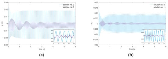
Figure 9.
Time series of a vibrating magnet close to the coil center at a frequency of = 75 rad/s and d = 0 m. (a) Magnet time response, (b) induced current time response. The blue color denotes the high energy solution (top branch) while purple means the low energy solution (bottom branch). The calculations were made for A = 0.001 m.
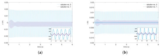
Figure 10.
Time series of a vibrating magnet close to the coil center at a frequency of = 75 rad/s and d = 0.016 m. (a) Magnet time response, (b) induced current time response. The blue color denotes the high energy solution (top branch) while purple means the low energy solution (bottom branch). The calculations were made for A = 0.001 m.
Analysis of the obtained time responses leads to the conclusion that the amplitudes of the magnet vibrations are very similar for d = 0 m and d = 0.016 m for the solution from the bottom and top branches. This confirmed the result from Figure 6a, where the resonance curves were overlapping, and the parameter d mainly influenced the resonance bandwidth.
The recovered current from the top branch and d = 0 m equals 0.0095 A (power of 0.9 W), while when setting d = 0.016 m the recovered current was 0.011 A (power of 1.21 W). This means that the shift of the magnet close to the coil’s end causes an increase in the harvested energy of 15%. Analyzing the results from the bottom branch, we may conclude that the recovered power can increase fourfold (from 0.01 W to 0.04 W) due to the magnet coil settings. To sum up, as it can be seen, the parameter d configurations produce different results in energy harvesting with a similar magnet vibration.
4.3. Bifurcation Analysis
Bifurcations mean topological changes in the parameter–dependent phase spaces. The nonlinear systems characterize multiplicity of solutions, hysteresis, amplitude jump and bifurcations. Therefore, bifurcation analysis is a very useful tool as it allows one to identify bifurcation points, stable and unstable regions and aids in the understanding of a nonlinear system.
As pointed out in Section 4.1, the magnet coil configuration may significantly modify the shape of the resonance curves and hysteresis effects. The bifurcation diagrams were made by a one–parameter and two–parameter continuation methods. Figure 11a,b show the bifurcation diagrams, depicted in , A) and (, A) space, for various parameters d and the frequency of excitation of = 70 rad/s. In these figures, the region with two stable solutions (continuous lines) and one unstable solution (dashed lines) are observed. When the magnet coil displacement is relatively small (d = 0 m), the multistability phenomenon occurs in the range of 0.00054–0.00092 m, for d = −0.008 m the multistability is observed for 0.00064–0.00095 m and for d = 0.016 m multistability is located for 0.00094–0.00114 m. Note that the magnet oscillations are practically the same outside the multistability area (Figure 11a). However, the bifurcation analysis shows that the recovered current differs in the total resonance region (Figure 11b). The loss of stability is caused by SNB points (circle points).
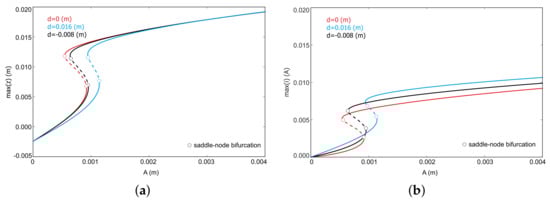
Figure 11.
One–parameter bifurcation diagrams for fixed excitation frequency of = 70 rad/s: (a) A versus maximal amplitude of the magnet, (b) A versus maximal induced current. The continuous and dashed lines show stable and unstable solutions, respectively. The circle means saddle-node bifurcations.
As the frequency increases to = 75 rad/s, the system’s multistability region is expanded (Figure 12). For the magnet coil configuration of d = 0 m the multistability appears for 0.00093–0.00207 m, for −0.008 m: 0.00093–0.00209 m and for d = 0.016 m: 0.00097–0.00219 m. Of course, after crossing the critical value of excitation 0.00114 m (for = 70 rad/s) and 0.00219 m (for = 75 rad/s) the harvester becomes monostable and only one solution appears.
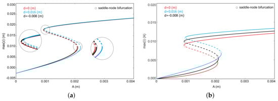
Figure 12.
One–parameter bifurcation diagrams for fixed excitation frequency of = 75 rad/s: (a) A versus maximal amplitude of the magnet, (b) A versus maximal induced current. The continuous and dashed lines show stable and unstable solutions, respectively. The circle means saddle-node bifurcations.
Analyzing the results in all bifurcation diagrams, we can conclude that the parameter d can be used to control (shift) the multistability region and improve the energy harvesting. It is possible to change the recovered energy without modifying the mechanical and electrical parameters. This is essential from a practical point of view.
Next, two–parameter continuation bifurcation diagrams obtained for the total resistance of R = 10 k (Figure 13a) and R = 20 k (Figure 13b) are presented. These diagrams are obtained when two parameters change simultaneously. In our case, the parameter d and frequency of excitation were chosen as varying. The numerical continuation starts from the SNB point for d = 0 m. The arrow shows the direction of the numerical continuation. The red line shows the subsequent locations of the SNB points in each step of simulation. The blue area shows the multistability region with two stable and one unstable solution(s).
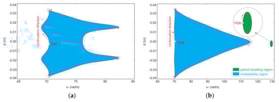
Figure 13.
Two–parameter continuation (, d) of saddle-node bifurcation (SNB) point: (a) the total resistance R = 10 k, (b) the total resistance R = 20 k. The continuation starts from the SNB point (or from the PDB point) obtained for d = 0 m (circle) and movement agrees with the arrows. The blue color means the region with two stable solutions, while the green area denotes the period doubling the bifurcation region. The red and black lines denote successive positions of SNB or PDB points, respectively. These plots were calculated for an amplitude of A = 0.001 m.
By analyzing the results in Figure 13a we can conclude that the multistability can be expanded from 70.5–76.5 rad/s for d = 0 m to 68–82 rad/s for d = −0.02 m. This means that we can easily extend the hardening effect and increase the amount of harvested energy. The blue region is symmetric and slightly shifted towards the negative values of parameter d due to the influence of gravity.
It is interesting that the situation is completely reversed if the resistance increases to R = 20 k (Figure 13b). Now, the multistability region is the widest for d = 0 m ( 70.115 rad/s). If the oscillating magnet moves away from the center of the coil, the area with two stable solutions strongly decreases. The critical values of the existence of multistability equals = 0.035 m and = −0.04 m. This result is clearly observed in the frequency–amplitude curves (Figure 14a). The red line denotes the harvester response for d = 0 m and the blue line means the response for d = 0.016 m. The nonlinear resonance is wider for d = 0 m. These obtained results signify that the multistability region depends on the resistance as well.
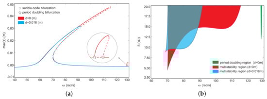
Figure 14.
Resonance curve and two-parameter continuation diagram for the maglev harvester. (a) Frequency–response curves obtained for the resistance R = 20 k. The red line shows the response for d = 0 m, the blue line for d = 0.016 m. (b) Two-parameter plot (R, ) showing the multistability region. The red color indicates the region obtained for d = 0 m, the blue region for d = 0.016 m. Interestingly, for higher frequencies, the small period-doubling region appears (green color). The calculations were made for A = 0.001 m.
Moreover, for higher resistance a new small resonance region (green color) close to the frequency of = 130 rad/s appears. This region exists only if the magnet oscillates close to the coil’s center. The response is caused by the period–doubling bifurcation PDB (Figure 14a). In this location, the magnet oscillation amplitude is very small, which suggests that experimental verification of the result will be difficult.
Finally, the two–parameter continuation of the resistance R and the frequency of excitation is presented in Figure 14b. This diagram unequivocally shows that the resistance affects the multistability region. Changing the position of the oscillating magnet in the coil extends the multistability area only within a certain range of resistance ( 0.9–1.45 k). For low resistance (below 0.9 k) the multistability occurs only for the magnet position d = 0 m. Below the value of R < 0.4 k the multistability disappears. For high resistance (above 15 k), the nonlinear resonance is wide 70–115 rad/s. Moreover, a small region of period–doubling (green area in Figure 14b) exists for resistance greater than 12 k close to the frequency of 128 rad/s.
Analysis of the basins of attraction for high levels of resistance leads to an interesting conclusion that the high energy output is much easier to obtain. Now, the nonlinear resonance is wider for d = 0 m and the probability of solution no. 2 reaches 70% (Figure 15a).
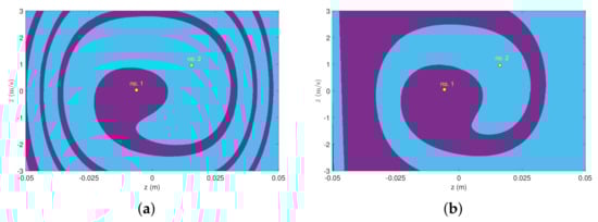
Figure 15.
Basins of attraction for the coexisting attractors for the frequency = 75 rad/s and resistance of R = 20 k, for (a) d = 0 m, (b) d = 0.016 m. Here, the purple regions are the basins of attraction with attractor no. 1 corresponding to the low energy harvesting and the blue region represents the basins of attraction with attractor no. 2 corresponding to the high energy harvesting. The probability of solution no. 2 decreases with a change in the magnet position from 70% (a) to 54% (b). The calculations were made for A = 0.001 m.
Moving the magnet closer to the edge of the induction coil causes the nonlinear resonance to become narrower (Figure 14b). However, the decrease in the probability of solution no. 2 is much less than the case of R = 10 k and equals 54% (Figure 15b). This is because increasing the resistance reduces the damping in the electrical system.
5. Conclusions
In this paper, an electromagnetic harvester with various models of electromechanical coupling was presented. The electromechanical coupling characterizes the conversion of vibration energy to electricity. Firstly, various models of the electromechanical coupling (constant value, linear and nonlinear functions) were proposed and compared with the experiment. In the nonlinear model, the position of the magnet oscillation in the coil was included. The obtained results lead to conclusions that the harvester with nonlinear electromechanical coupling model is closest to the experimental response. As shown, the classical modeling of the electromechanical coupling (constant value or linear function) can be also accepted for small magnet oscillations. In our system, for magnet amplitudes higher than 0.01 m the nonlinear electromechanical coupling model should be applied. Due to this, for detailed analysis, the nonlinear electromechanical model was chosen.
The nonlinear model of the electromechanical coupling includes a parameter that describes the position of the oscillating magnet in the coil. The nonlinear resonance and recovered energy can be simply controlled by this parameter. With the help of this parameter the shape of the resonance curves and the multistability can be modified. In the multistability region, two stable and one unstable solution(s) appear, and one of these solutions is characterized by a much greater level of energy recovery (even two and a half times more).
However, the shift of the magnet close to the coil’s end causes difficulties in obtaining the high energy output. The basin of attraction (i.e., the set of initial conditions) for the high energy output is significantly reduced. The probability of the high energy solution close to the coil’s center equals 42%, while in the vicinity of the coil’s end it is only 6%.
Another solution is obtained with the increase in the load resistance. Then, the best magnet position is close to the coil’s center (Figure 13b) and the probability is very high (70%, Figure 15a). However, the magnet shift for this resistance causes the nonlinear resonance to be reduced but the decrease in the probability of the high output solution is smaller (54%, Figure 15b). Moreover, for a higher range of resistance, a new solution caused by period bifurcation is detected.
Summarizing, the shift of the position of vibration of the magnet in the coil improves the nonlinear resonance only within a certain range of resistance (Figure 14b). The detailed bifurcation analysis shows that the multistability region can easily be controlled by the resistance and the proper configuration of the magnet coil components.
Author Contributions
Conceptualization, K.K.; methodology, K.K; software, K.K.; validation, K.K.; investigation, K.K. and M.K.; writing—review and editing, K.K. and M.K.; visualization, K.K.; supervision, K.K.; funding acquisition, K.K. All authors have read and agreed to the published version of the manuscript.
Funding
This research was financed in the framework of the project “Theoretical–experimental analysis possibility of electromechanical coupling shaping in energy harvesting systems” no. DEC−2019/ 35/B/ST8/01068, funded by the National Science Centre, Poland.
Institutional Review Board Statement
Not applicable.
Informed Consent Statement
Not applicable.
Acknowledgments
We would like thank to the A. Teter for helpful discussions.
Conflicts of Interest
The authors declare no conflict of interest.
Abbreviations
The following abbreviations are used in this manuscript:
| EH | energy harvesting |
| ES | energy scavening |
| VEHs | vibration energy harvesters |
| EC | electromechanical coupling |
| SNB | saddle−node bifurcation |
| PDB | period doubling bifurcation |
References
- Fagas, G.; Gallagher, J.P.; Gammaitoni, L.; Paul, D.J. Energy Challenges for ICT. In ICT—Energy Concepts for Energy Efficiency and Sustainability; Fagas, G., Gammaitoni, L., Gallagher, J.P., Paul, D.J., Eds.; InTechOpen: London, UK, 2017; pp. 1–36. [Google Scholar]
- Park, H.; Lee, D.; Park, G.; Park, S.; Khan, S.; Kim, J.; Kim, W. Energy harvesting using thermoelectricity for IoT (Internet of Things) and E-skin sensors. J. Phys. Energy 2019, 1, 042001. [Google Scholar] [CrossRef]
- Elaji, M.; Munir, K.; Eugeni, M.; Atek, S.; Gaudenzi, P. Energy Harvesting towards Self-Powered IoT Devices. Energies 2020, 13, 5528. [Google Scholar]
- Yunus, N.H.M.; Sampe, J.; Yunas, J.; Pawi, A.; Rhazali, Z.A. MEMS based antenna of energy harvester for wireless sensor node. Microsyst. Technol. 2020, 26, 2785–2792. [Google Scholar] [CrossRef]
- Butt, Z.; Rahman, S.U.; Pasha, R.A.; Mehmood, S.; Abbas, S.; Elahi, H. Characterizing barium titanate piezoelectric material using the finite element method. Trans. Electr. Electron. Mater. 2017, 18, 163–168. [Google Scholar]
- Swati, R.; Elahi, H.; Wen, L.; Khan, A.; Shad, S.; Mughal, M.R. Investigation of tensile and in-plane shear properties of carbon fiber reinforced composites with and without piezoelectric patches for micro-crack propagation using extended finite element method. Microsyst. Technol. 2019, 25, 2361–2370. [Google Scholar] [CrossRef]
- Mitcheson, P.D.; Yeatman, E.M.; Rao, G.K.; Holmes, A.S.; Green, T.C. Energy harvesting from human and machine motion for wireless electronic devices. Proc. IEEE 2008, 96, 1457–14861. [Google Scholar] [CrossRef]
- Wang, W.; Cao, J.; Zhang, N.; Li, J.; Liao, W.H. Magnetic-spring based energy harvesting from human motions: Design, modeling and experiments. Energ. Convers. Manag. 2017, 132, 189–197. [Google Scholar] [CrossRef]
- Rajarathinam, M.; Ali, S.F. Energy generation in a hybrid harvester under harmonic excitation. Energ. Convers. Manag. 2018, 155, 10–19. [Google Scholar] [CrossRef]
- Zhang, Y.; Cao, J.; Zhu, H.; Lei, Y. Design, modeling and experimental verification of circular Halbach electromagnetic energy harvesting from bearing motion. Energ. Convers. Manag. 2019, 150, 811–821. [Google Scholar] [CrossRef]
- Saha, C.R.; O’Donnel, T.; Wang, N.; Mc Closkey, P. Electromagnetic generator for harvesting energy from human motion. Sens. Actuators A Phys. 2008, 147, 248–253. [Google Scholar] [CrossRef]
- Rome, L.C.; Flynn, L.; Goldman, E.M.; Yoo, T.D. Generating electricity while walking with loads. Science 2005, 3090, 1725–1728. [Google Scholar] [CrossRef]
- Ni, T.; Zuo, L.; Kareem, A. Assessment of energy potential and vibration mitigation of regenerative tuned mass dampers on wind excited tall buildings. In Proceedings of the ASME 2011 International Design Engineering Technical Conferences and Computers and Information in Engineering Conference, Washington, DC, USA, 28–31 August 2011; pp. 333–342. [Google Scholar]
- Zuo, L.; Scully, B.; Shestani, J.; Zhou, Y. Design and characterization of an electromagnetic energy harvester for vehicle suspensions. Smart Mater. Struct. 2010, 19, 045003. [Google Scholar] [CrossRef]
- Nagode, C.; Ahmadian, M.; Taheri, S. Effective energy harvesting devices for railroad applications. In Proceedings of the SPIE Smart Structures and Materials + Nondestructive Evaluation and Health Monitoring, Active and Passive Smart Structures and Integrated Systems; SPIE: San Diego, CA, USA, 2010; Volume 76430X. [Google Scholar]
- Choi, Y.T.; Wereley, N.M. Self-powered magnetorheological dampers. J. Vib. Acoust. 2009, 131, 044501. [Google Scholar] [CrossRef]
- Scruggs, J.T.; Lattanzio, S.M.; Taanidis, A.A. Optimal causal control of a wave energy converter in a random sea. Appl. Ocean Res. 2013, 42, 1–15. [Google Scholar] [CrossRef]
- Rhinefrank, K.; Agamloh, E.B.; Von Jouanne, A.; Wallace, A.K.; Prudell, J.; Kimble, K.; Aills, J.; Schmidt, E.; Chan, P.; Sweeny, B.; et al. Novel ocean energy permanent magnet linear generator buoy. Renew. Energy 2006, 31, 1279–1298. [Google Scholar] [CrossRef]
- Masoumi, M.; Wang, Y. Repulsive magnetic levitation-based ocean wave energy harvester with variable resonance: Modeling, simulation and experiment. J. Sound Vib. 2016, 381, 192–205. [Google Scholar] [CrossRef]
- Zuo, L.; Tang, X. Large-scale vibration energy harvesting. J. Intell. Mater. Syst. Struct. 2013, 24, 1405–1430. [Google Scholar] [CrossRef]
- Saravia, C.M.; Ramirez, J.M.; Gatti, C.G. A hybrid numerical-analytical approach for modeling levitation based vibration energy harvesters. Sens. Actuators A Phys. 2017, 257, 20–29. [Google Scholar] [CrossRef]
- Munaz, A.; Lee, B.C.; Chuang, G.S. A study of an electromagnetic energy harvester using multi-pole magnet. Sens. Actuators A Phys. 2013, 201, 134–140. [Google Scholar] [CrossRef]
- Glynne-Jones, P.; Tudor, M.J.; Beeby, S.P.; White, N.M. An electromagnetic, vibration-powered generator for intelligent sensor systems. Sens. Actuators A Phys. 2004, 110, 344–349. [Google Scholar] [CrossRef]
- Stephen, N.G. On energy harvesting from ambient vibration. J. Sound Vib. 2006, 293, 409–425. [Google Scholar] [CrossRef]
- Camarano, A.; Neild, S.A.; Burrow, S.G.; Wagg, D.J.; Inman, D.J. Optimum resistive loads for vibration-based electromagnetic energy harvesters with a stittening nonlinearity. J. Intell. Mater. Syst. Struct. 2014, 25, 1757–1770. [Google Scholar] [CrossRef]
- Mann, B.P.; Sims, N.D. Energy harvesting from the nonlinear oscillations of magnetic levitation. J. Sound Vib. 2009, 319, 515–530. [Google Scholar] [CrossRef]
- Zhu, Y.; Zu, J.W.; Guo, L. A magnetoelectric generator for energy harvesting from the vibration of magnetic levitation. IEEE Trans. Magn. 2012, 48, 3344–3347. [Google Scholar] [CrossRef]
- Lee, H.; Noh, M.D.; Park, Y.W. Optimal design of electromagnetic energy harvester using analytic equations. IEEE Trans. Magn. 2017, 53, 8207605. [Google Scholar] [CrossRef]
- Bernal, A.G.A.; Garcia, L.E.L. The modelling of an electromagnetic energy harvesting architecture. Appl. Math. Model. 2012, 36, 4728–4741. [Google Scholar] [CrossRef]
- Dos Santos, M.P.S.; Ferreira, J.A.F.; Simoes, J.A.O.; Pascoal, R.; Torrao, J.; Xue, X.; Furlani, E.P. Magnetic levitation-based electromagnetic energy harvesting: A semi-analytical non-linear model for energy transduction. Sci. Rep. 2016, 6, 18579. [Google Scholar] [CrossRef]
- Saravia, M.M. On the electromechanical coupling in electromagnetic vibration energy harvesters. Mech. Syst. Signal Process. 2020, 136, 106027. [Google Scholar] [CrossRef]
- Kecik, K.; Mitura, A.; Lenci, S.; Warminski, J. Energy harvesting from a magnetic levitation system. Int. J. Non-Linear Mech. 2017, 94, 200–206. [Google Scholar] [CrossRef]
- Kecik, K. Architecture and optimization of a low-frequency maglev energy harvester. Int. J. Struct. Stab. 2019, 19, 1950097. [Google Scholar] [CrossRef]
- Berdy, D.F.; Valentino, D.J.; Peroulis, D. Design and optimization of a magnetically sprung block magnet vibration energy harvester. Sens. Actuators A Phys. 2014, 218, 69–79. [Google Scholar] [CrossRef]
- Constantinou, P.; Mellor, P.H.; Wilcox, P.D. A magnetically Sprung Generator for Energy Harvesting Applications. IEEE/ASME Trans. Mechatron. 2012, 17, 415–424. [Google Scholar] [CrossRef]
- Mosch, M.; Fischerauer, G. A comparison of methods to measure the coupling coefficient of electromagnetic vibration energy harvesters. Micromachines 2019, 10, 826. [Google Scholar] [CrossRef]
- Carneiro, P.; dos Santos, M.P.S.; Rodrigues, A.; Ferreira, J.A.F.; Simoes, J.A.O.; Torres Marques, A.; Kholkin, A.L. Electromagnetic energy harvesting using magnetic levitation architectures: A review. Appl. Energy 2020, 260, 114191. [Google Scholar] [CrossRef]
- Kecik, K. Dynamics and control of an active pendulum system. Int. J. Non-Linear Mech. 2015, 70, 63–67. [Google Scholar] [CrossRef]
- Kecik, K.; Mitura, A. Theoretical and experimental investigations of a pseudo-magnetic levitation system for energy harvesting. Sensors 2015, 20, 1623. [Google Scholar] [CrossRef]
- Doedel, E.; Oldeman, B. Dynamics: Auto-07p: Continuation and Bifurcation Software for Ordinary Differential Equations; Concordia University Montreal: Montreal, QC, Canada, 2012. [Google Scholar]
- Nusse, H.E.; Yorke, J.A.; Kostelich, J. Dynamics: Numerical Explorations; Springer: New York, NY, USA, 1994. [Google Scholar]
Publisher’s Note: MDPI stays neutral with regard to jurisdictional claims in published maps and institutional affiliations. |
© 2021 by the authors. Licensee MDPI, Basel, Switzerland. This article is an open access article distributed under the terms and conditions of the Creative Commons Attribution (CC BY) license (https://creativecommons.org/licenses/by/4.0/).