Abstract
This article presents a method for detecting defects and assessing their size in soft magnetic composites (SMCs) based on magnetograms obtained from a magnetic field camera and a numerical analysis of the magnetic field around them. For the purpose of the experiment, toroidal samples of a metal–polymer composite were made, in which holes and gaps simulating defects were prepared. The magnetic camera allowed for registering the magnetic flux density image near the surface of the samples. As a result, magnetograms with information about the location and geometry of defects were obtained. A numerical analysis was used to investigate the influence of various factors, such as defect depth, its size and material permeability. Theoretical changes in magnetic field over defects stay in good agreement with measurements, which is a strong indication that surface field magnetograms can be useful in a quality assessment of the considered composites. The effectiveness and usefulness of the method in detecting surface and shallow subsurface defects in SMC materials was confirmed. The influence of a possible tangent component of the exciting field was demonstrated and discussed.
1. Introduction
Constant development in the electronics and electrical industry poses a challenge for scientists and engineers developing modern materials. As a result, one of the developed solutions is the improvement and introduction of new technologies for the processing of metal–polymer composites. End users expect the materials to exhibit appropriate mechanical and physical properties suitable for a specific application. Apart from choosing the optimal composition of the product and its processing route, it is also important to control the quality of finished products. Such a process must be adapted to various shapes of the products. It also has to ensure the appropriate speed and accuracy of the controls. For this purpose, one or a combination of many non-destructive tests (NDTs) may be used. NDTs are particularly useful as cost-effective inspection methods in many manufacturing processes. Applications of a wide spectrum of NDTs can be found in works of many researchers. Gholizadeh [1] described a series of NDTs and pointed out the important role they play in the testing of composite materials. Seifi et al. [2] described the role and importance of quality verification methods in metal additive manufacturing. Hufenbach et al. [3] analyzed many problems appearing during repeated acceptance checks of pressure vessels and pipelines. In the case of composite materials for the aerospace industry, a review of X-ray imaging techniques was presented by Jandejsek et al. [4]. Fotsing et al. [5] presented an optical system based on deflectometry for the measurement and quantification of surface defects in sandwich-type composites.
Composite materials, especially magnetically soft ones, are the subject of numerous research and development works. Soft magnetic composites (SMCs) are used, inter alia, in transformers and electrical devices, due to the possibility of forming magnetic circuits of complex shapes and lower losses (compared to steel laminates) at higher frequencies [6]. These useful features find particular application in the construction of electric vehicles and the electric motors driving them with high power density [7]. Schoppa and Delarbre [8] pointed out that composites made of soft magnetic powders allow for the construction of complex three-dimensional magnetic cores, with magnetization topology unattainable for traditional laminated sheets. SMCs offer optimal magnetic properties at higher operating frequencies and contribute to an increase in power density in miniature electric machines. Through appropriate selection of the composite and the method of its processing, the physical and chemical properties of SMCs can be adapted to specific applications, with a relatively small amount of work and costs.
The final properties of SMC cores are influenced not only by the properties of the bulk material but also by the occurrence of hidden flaws, which is why the issue of material research and diagnostics has become key. Non-destructive methods are aimed at detecting both volumetric and surface defects. There are many NDTs based on various physical phenomena, like acoustic waves, ultrasonics, active thermography and magnetic methods, for example [9,10,11]. On the other hand, some of the aforementioned methods reveal severe limitations; it is, for example, necessary to scan large areas of the structure in order to characterize relatively small defects. In acoustic wave methods, the collected data from many sensors have a complex amplitude distribution, often with overlapping areas. This causes difficulties in identifying and distinguishing defects. The acoustic waves and ultrasonics methods require contact of sensors with the tested material. In addition, during the measurements, the impedance matching of the measured material and the material from which the sensors are made should be taken into account. This significantly complicates the measuring system when determining details of different qualitative and quantitative composition. Methods that do not require direct contact with the tested material, such as active thermography and magnetic methods, do not have such limitations. These two families of methods have many things in common. They enable the detection of defects mainly on the surface or close to the surface of the sample. It depends on the depth of penetration of the electromagnetic wave (in particular, infrared), as well as the difference between the bulk and defect material properties. The resolution of the defect image depends on the resolution of the apparatus used. Additionally, in the case of active thermography, the obtained results may be affected by ambient temperature and reflections. There is also a risk that the sudden delivery of energy to heat the test object will create stresses due to thermal expansion. An example of the use of active thermography to detect inclusions in a composite material was the subject of one of the author’s earlier considerations [12].
Classical magnetic methods, such as eddy-current testing and magnetic flux leakage (MFL) testing, struggle with limitations such as low resolution of measurements and the need to use a large number of sensors (often large and inconvenient to use) [13], and are currently not widely used in measurements of assessment of SMCs’ structure homogeneity. It should also be noted that SMC materials have very low eddy current losses, which further reduces the effectiveness of methods based on eddy currents. On the other hand, MFL testing is mainly used to test ferromagnetic materials such as pipelines [14] and permanent magnets in electrical machines [15]. The MFL method is based on applying a magnetic field tangentially to the tested ferromagnetic surface. It is especially effective in detecting defects perpendicular to the applied magnetic field, as magnetic flux then leaks out of the tested material.
To solve the problem of low defect image resolution, some authors suggested the application of arrays of tiny probes sweeping small areas of interest. Boero et al. [16] provided a review of performance, technology and theoretical foundations, as well as applications of micro-Hall sensor arrays for NDT purposes. Smith and Harrison [17] focused on the possibility of performing rapid large area tests with such sensor arrays using a transient eddy current excitation. They concluded that it is possible to automate the scanning process with a 10-times increased speed compared to single sensor probe. Janousek et al. [18] investigated the impact of excitation frequency on resonance in the gap (material damage). Kosmas et al. [19] presented a prototype of a Hall sensor for non-destructive testing of ferromagnetic surfaces. The sensor enabled the detection of magnetic anomalies due to various gaps or cracks in the stack of laminated sheets.
Based on previous experiences [20], this article proposes to develop the previously described methods of magnetic NDT methods. Magnetic field distribution on the surface of an SMC is examined with the use of a camera with matrix of micro-Hall sensors. The analysis of magnetograms allows one to detect surface and subsurface material defects in SMCs. The experimental studies are supported with analytical description and numerical analysis. The advantage of the proposed method is that it relies on the speed, high resolution and reliability of anomaly detection; thus, the method can be used wherever speed is an important factor, e.g., various stages of SMC circuit production.
2. Materials and Methods
2.1. Preparation of Samples
For the purpose of the research task, toroidal samples were prepared based on metal–polymer powder compositions. Possibilities for producing self-made SMC cores using easily available powder components, mainly iron and polyvinyl chloride (PVC), are presented in [21]. The magnetic properties achieved are comparable with MnZn ferrites and, therefore, the composites can be used in similar applications, e.g., filters suppressing electromagnetic interference, chokes, matching transformers of small size. As a result of further development works, the properties of the obtained cores were improved. Ultimately, as a result of experimental research, it was found that the best magnetic parameters in quasi-static conditions could be obtained using a grain size in the range of 100–150 μm, 0.5% PVC content, a forming pressure of about 500 MPa and a forming temperature in the range of 170–180 °C [21]. The toroidal samples with a rectangular cross-section had an outer diameter of 50 mm, an inner diameter of 30 mm, a height of 10 mm and a weight of 79.5 g. Specimens and molding press is shown in Figure 1.
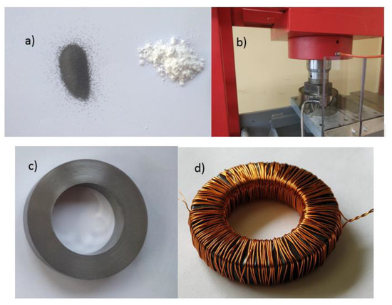
Figure 1.
Illustrative steps in the production of composite core samples: (a) components, (b) forming, (c) produced core, (d) core with windings.
2.2. Magnetic Parameters
The magnetic parameters of the samples were measured using the REMACOMP C-200 computer measuring system. The scheme is shown in Figure 2. The measurement methodology applied to the apparatus complies with the IEC 60404 standard. The measuring shunt R was used to measure the magnetizing current and the primary circle voltage drop. Based on this, the H magnetic field strengths were determined. Fast A/D converters were responsible for voltage sampling on the secondary circle. The digital signal was then integrated to compute magnetic flux density B, which allowed us to obtain the mean B(H) curve (Figure 3), loss or transmittance values. The values of characteristic parameters describing the B(H) curve of the tested samples at a frequency of 10 Hz were as follows: remanence Br = 0.35 T, coercivity Hc = 400 A/m, saturation Bmax = 1.3 T, Hmax = 6700 A/m, relative permeability µrmax = 400 at H ≈ 1020 A/m.
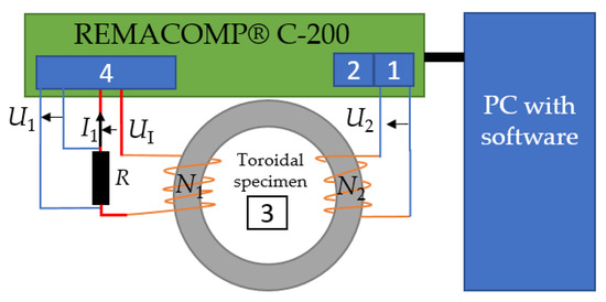
Figure 2.
The REMACOMP® C-200 system (own work based on [22]): 1—programmable signal generator, 2—power amplifier, 3—tested toroidal core, 4—digital sampling system with preamplifiers and A/D converter, N1 and N2—primary and secondary windings.
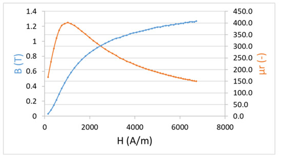
Figure 3.
Typical B(H) curve and relative permeability μr for own produced SMC cores used in tests.
2.3. Defects
In order to simulate defects, some holes or cuts were made in the samples. A CNC machine was used to drill holes of the same diameter of 2 mm but at different depths (2, 3, 4, 5, 6, 7 mm) in sample A1 (Figure 4a), and holes of the same depth (2 mm) but different diameters (2, 3, 4, 5 mm) in sample A2 (Figure 4b). A 0.6 mm gap was cut in sample A3 using a waterjet cutter (Figure 4c).
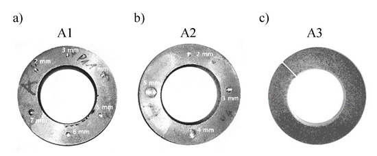
Figure 4.
Samples with prepared defects: (a) sample A1 with holes of various depths and a diameter of 2 mm; (b) sample A2 with holes of various diameters and a depth of 2 mm; (c) sample A3 with a 0.6 mm cut in an angular plane.
2.4. Measurements
The measurement idea is shown in Figure 5. The sample was placed on a permanent magnet VMM4-N35 (cylinder with dimensions: diameter 55 mm, height 15 mm) and separated from it with a paper divider. As the magnetic force of the permanent magnet was 510 N, it was necessary to use a spacer to facilitate the disengagement of the elements. The magnetic field on the top core surface was detected with a Hall sensor array built in the commercial product, namely the MagCam 3D camera (see Vervacke [23] and Nishio et al. [24] for a more detailed description of the measurement concept).
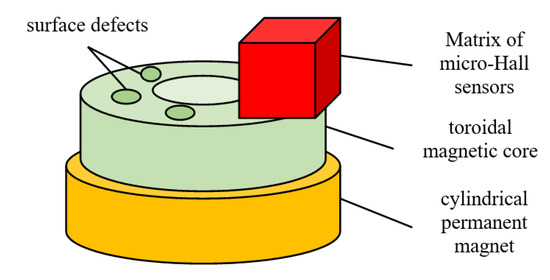
Figure 5.
Measurement idea.
MagCam (Figure 6) was designed to determine the Cartesian components of magnetic flux density. Then, via elementary vector analysis, the B field components in cylindrical or spherical coordinates could be found. An array of 128 × 128 micro-Hall sensors covered an area of 12.7 mm × 12.7 mm, with a resolution of 0.1 mm. The Magnetic field range was ±1 T at a resolution of 0.2 mT. Each of the Hall sensors had an active area of 40 μm × 40 μm.
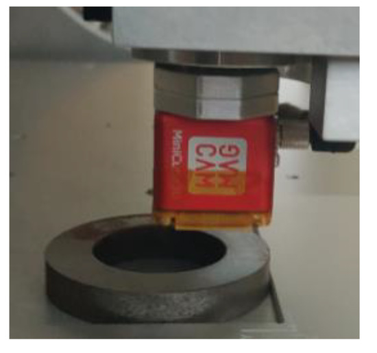
Figure 6.
MiniCube3D three-axis magnetic field camera (MagCam).
2.5. Governing Equations and Numerical Simulations
Static magnetic field satisfies the following equations:
where is magnetic flux density, is the total current density and is the magnetic permittivity of vacuum. In matter, it is convenient to divide the total currents into two groups: those related to electric charge movement across the medium and those related to matter structure. The first are called the free currents (of density ), whereas the latter are the bound currents (of density ). The bound currents originate from magnetic moments of subatomic components of matter, such as electrons. The volumetric density of these moments, , is called the magnetization, and is related to the bound currents’ density with relationship , so that the first Equation (1) becomes
where
is the magnetic field intensity. In magnetic materials, magnetization is a function of many factors, including or fields, and often manifests hysteresis. In this paper, we will assume the magnetization in the magnet is constant (), whereas it is proportional to the magnetic field in other regions: , so that Equation (3) can be rewritten as follows
where is the effective magnetic permeability of the medium.
In order to find what can be expected and to explain the observed effects, a series of numerical tests were performed with the use of finite elements. During calculations, various values of defect dimensions, shape and material relative permeability were used. To speed up the calculations, the defects were modeled in simplified forms allowing a use of 2D calculations (FEMM software was used). In case of cylinder shaped defects (holes), axial symmetry was assumed nearby the hole, which allowed calculations in (r, z) the coordinate system (Figure 7). The basic parameters of the hole are its depth (d) and diameter (D).
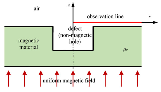
Figure 7.
Non-magnetic hole in magnetic material; magnetic flux density was calculated at points on the observation line (red).
Preliminary numerical simulations with various values of parameters showed a very sharp peak of magnetic flux density nearby the hole edge. Taking into account that realistic holes prepared in the composite do not have such sharp edges, two versions of smoother edges were also considered: with round edge and with beveled edge. All three versions of hole profiles are presented in Figure 8.
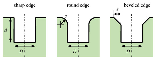
Figure 8.
Variants of holes in magnetic material: d—hole depth, D—hole diameter, s—edge radius or bevel.
The second tested defect was a cut across the magnetic material. The configuration is presented in Figure 9. The main parameters are cut width w and material permeability but, to explain observations, it was necessary to introduce round edges and tilt of source field vector (angle α).
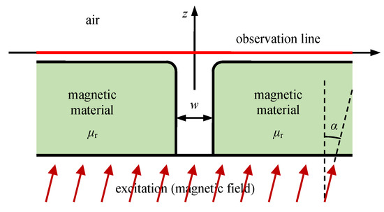
Figure 9.
Modeled cut of magnetic material: w—gap width, α—tilt of source magnetic field vector.
In each simulation, the magnetic flux density components were calculated on the observation line (thick red lines in Figure 7 and Figure 9), which was practically on the surface of the magnetic material. The results of calculations are presented in relative form as Bz/Bz0 or Br/B0, where B0 and Bz0 are the magnitude and the z component of the B field, respectively, above the defect location when the defect is absent.
3. Results and Discussion
3.1. Simulation Results for Cylinder Shaped Holes
Figure 10 presents the distribution of magnetic flux density (z component) on the observation line for various values of material permeability and constant depth (d = 2 mm), and the diameter (D = 2 mm) for the sharp edge of the hole (s = 0). Even for relatively small values of μr, the field distortion is clearly visible. The traces for μr > 10 are almost the same. This means even defects in weak magnetic materials should be detectable.
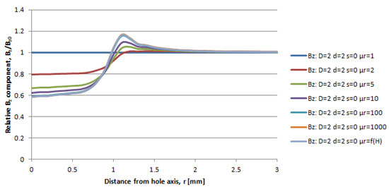
Figure 10.
Magnetic flux density (z component) on the observation line for various values of relative permeability of the material (μr) and hole diameter D = 2 mm, depth d = 2 mm, sharp edge; traces for μr > 10 are practically the same; therefore, only one is visible; μr = f(H) stands for the characteristic given in Figure 3.
The effect of the hole edge smoothness expressed by parameter s is shown in Figure 11. The sharp edge produces a sharp peak over the edge (green trace). Beveling the edge (brown and blue traces) shifts the peak outside, keeping its value nearly at the same level. As a result, this effectively enlarges the hole diameter. The round edge smooths the peak and slightly enlarges the effective hole diameter (see violet and cyan traces). When compared with the measured values, which are presented in Section 3.2, the trace with the round edge seems to best match the measured values. Therefore, further results of simulations are limited to those for the round edge with s = 0.5 mm, which seems more realistic than an ideally sharp edge.
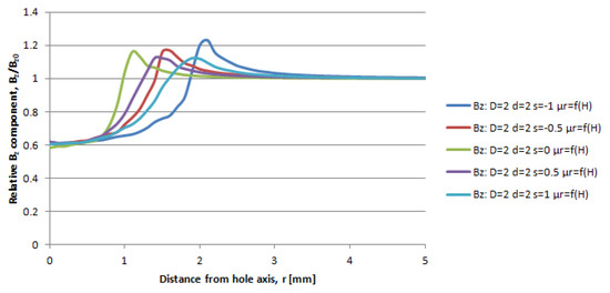
Figure 11.
Magnetic flux density (z component) on the observation line for various hole edge smoothness and hole diameter D = 2 mm, depth d = 2 mm, material relative permeability μr given in Figure 3; the hole smoothness is expressed by parameter s: 0—sharp edge, s > 0—round edge of radius equal to s mm, s < 0—beveled edge with bevel equal to -s mm.
Figure 12 shows the effect of hole depth. It follows that, even a hole of a small depth significantly changes the field, both the axial and radial components. Therefore, all such defects can be easily detected. However, the values of magnetic field on the observation line are practically the same for depths larger than around 1 mm. Therefore, this method can detect the defect, but it cannot reliably detect its depth.
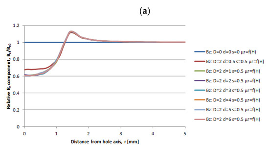
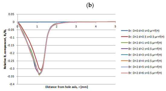
Figure 12.
Magnetic flux density ((a) z component; (b) r component) on the observation line for various values of hole depth and hole diameter D = 2 mm, round edge s = 0.5 mm and magnetic material of B(H) curve given in Figure 3; traces for depths larger than 1 mm are practically the same.
Figure 13 shows the effect of the hole diameter. The larger diameter, the larger the distance between the peak and hole axis. Moreover, the larger the diameter, the larger the peak and the deeper the minimum. Hence, different diameters result in different traces, which makes it possible to identify the hole diameter.
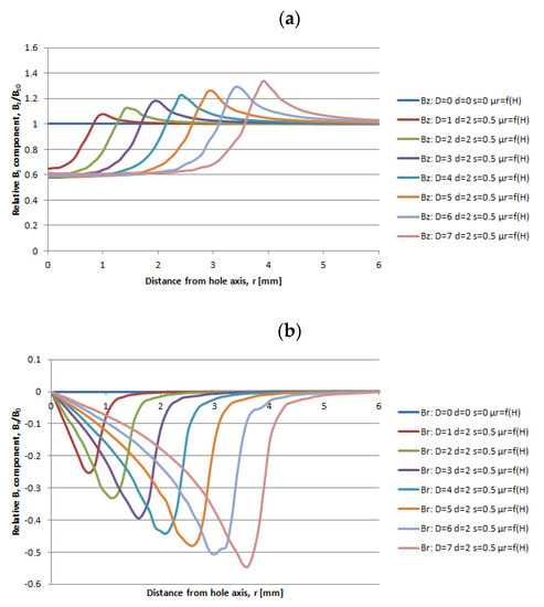
Figure 13.
Magnetic flux density ((a) z component; (b) r component) on the observation line for various values of hole diameter and hole depth d = 2 mm, round edge s = 0.5 mm and magnetic material of B(H) curve given in Figure 3.
3.2. Measurement Results for Holes of Various Depths
Figure 14 shows a magnetogram of sample A1. It clearly reveals the drilled holes. The 7 mm hole seems much larger due to accidental damage of the surface near the hole. The magnetogram shows the positions of the holes; however, it is hard to assess the depth of the holes.
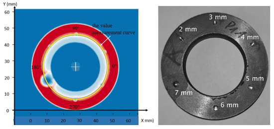
Figure 14.
Magnetogram of sample A1 with the sample view.
A more detailed picture of qualitative and quantitative defect features is shown in Figure 15. It shows the field distribution along the observation line marked in Figure 14 (a circle of a radius around 20 mm on the sample surface). In this approach, it seems possible to estimate both the surface area and the depth of the hole. However, the differences between the field values nearby particular holes are small. This stays in agreement with the results presented in Section 3.1 (see Figure 12 and related comment). The information presented in Figure 15 is supplemented with data in Table 1, which shows the minimum values of B field related to each hole. The magnetic flux density slightly decreases with the depth of the hole. The correlation coefficient between minimum B field and hole depth equals −0.74 (with exclusion of the damaged 7 mm hole). Small deviations from the trend can be a result of imperfect alignment of the holes, which causes the observation curve to not run exactly through the middle of each hole (see Figure 14).
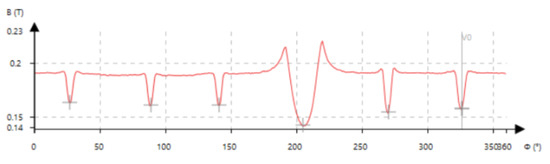
Figure 15.
Distribution of magnetic flux density form on sample A1 along the observation curve shown in Figure 14.

Table 1.
Minimum values of flux density B related to holes of sample A1.
3.3. Measurement Results for Holes of Various Diameters
Figure 16 shows a magnetogram of sample A2. The holes are clearly visible and their sizes can be easily assessed. Figure 17 shows the plot of magnetic flux density (z component) along the observation contour shown in Figure 16. This time, the shape and size of the field plot nearby the holes can be clearly connected with its diameter, which stays in agreement with results presented in Section 3.1 (see Figure 13). The information on B minima is presented in Table 2. The value of field B clearly decreases as the diameter of the holes increases. The correlation coefficient between minimum B field and hole diameter was −0.98.
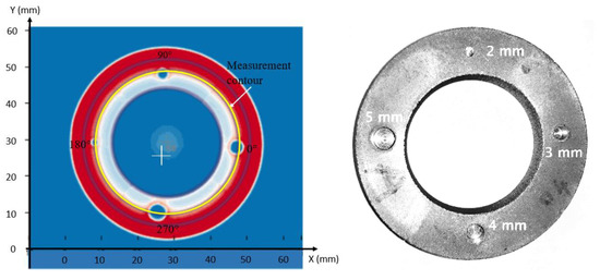
Figure 16.
Magnetogram of sample A2 with the sample view.
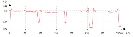
Figure 17.
Distribution of magnetic flux density (z component) along observation contour shown in Figure 12 for sample A2.
Table 2.
Minima of B field connected with holes in sample A2.
3.4. Simulation Results for Cut Shaped Defect
Figure 18 shows the z and x components of the B field on the observation line for a gap width of w = 0.6 mm and the magnetic permeability of material μr given in Figure 3. Round edges with s = 0.5 mm were used. When the source field tilt is 0°, the distribution is symmetrical with respect to the symmetry axis of the cut. The presence of the tangential component in the magnetizing field (represented by the tilt) leads to asymmetry. As the tilt increases, the asymmetry is more visible.
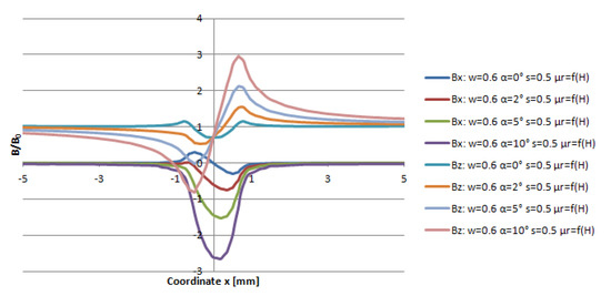
Figure 18.
Magnetic flux density (x and z components) on the observation line over the cut for a gap width of w = 0.6 mm, round edge s = 0.5 mm and magnetic permeability μr given in Figure 3.
Figure 19 shows the z component of the B field on the observation line for various magnetic permeability for a width of 0.6 mm and a tilt of α = 2°. The asymmetry of the field distribution rises with an increase in magnetic permeability. Low values of lead to clearly different shapes. As in the case of cylindrical defects, the traces for μr around 100 and higher are practically the same. This means that similar defects can be easily detected, even in magnetic materials of relatively low permeability.
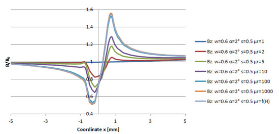
Figure 19.
Magnetic flux density (z component) on the observation line for various values of relative permeability of the material (μr), and a gap width of w = 0.6 mm, round edge s = 0.5 mm, source field tilt α = 2°; traces for μr ≥ 100 are practically the same; therefore, only one is visible; μr = f(H) stands for the characteristic given in Figure 3.
3.5. Measurement Results for Cut Shaped Defect
Figure 20 shows a 2D magnetogram for sample A3 with a 0.6 mm width of the gap. The magnetogram reveals the prepared cut. In the air gap, an abrupt jump of magnetic induction on exactly the crack position was observed. The jump is more visible in Figure 21, with a magnetic flux density distribution (z component) along a mean circumference (r = 20 mm). Table 3 presents more details on the peak in sample A3.
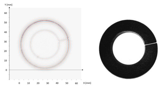
Figure 20.
Three-dimensional magnetogram of sample A3 with a visible cut.
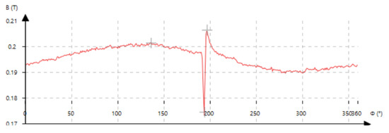
Figure 21.
B field (axial component) distribution vs. angle in sample A3 (gap 0.6 mm).
Table 3.
Characteristic values of magnetic flux density B nearby the cut in sample A3.
It is worth mentioning that the jump is asymmetrical. If the magnetizing field was ideally vertical (tilt α = 0°) and uniform, and the sample was ideally homogenous, the jump would be symmetrical, as shown in Figure 18 by blue trace for Bz and α = 0°. However, this is not the case. First of all, it should be taken into account that the magnetic field produced by the cylindrical magnet is not uniform. The radial and axial components of the magnet of constant magnetization can be found in [25]—let us denote them by and , respectively. Due to axial symmetry, no angular component is present, and the fields depend only on radial () and axial () coordinates. The inset visible in Figure 22 shows the typical distribution of magnetic field lines (blue arrowed lines) of a cylindrical magnet (orange rectangle). The distribution of , and total field along the thick black line on the magnet surface is shown in the main part of the figure. It is worth noting that the radial component (blue trace in Figure 22) varies rapidly near the magnet edge. As shown below, it has a great impact on the asymmetry near the cut-like defect.
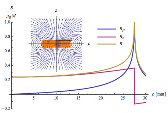
Figure 22.
Magnetic field density on the top surface of the cylindrical magnet (black line in the inset) vs. distance from the magnet axis; magnet diameter is 55 mm, magnet height is 15 mm, uniform magnetization, .
Suppose now that the sample and magnet -axes do not cover but are shifted by the certain distance . Let the mean radius of the observation contour (circle) equal (see Figure 23). Elementary vector analysis leads to the following expressions for the magnetic field density on the observation circle:
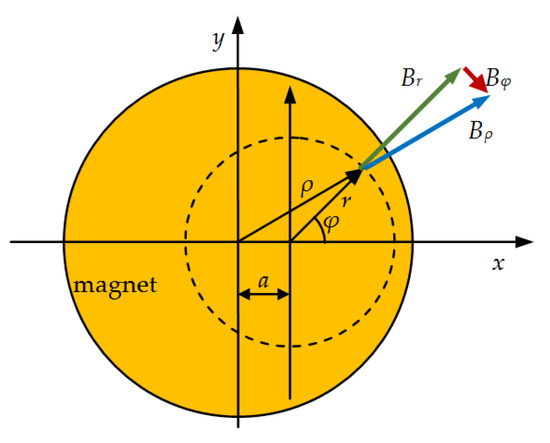
Figure 23.
Eccentric circle of radius r on the magnet’s surface.
It means that the magnetic field along the circle will also have a non-zero angular component , and axial component will vary with angle , as shown in Figure 24.
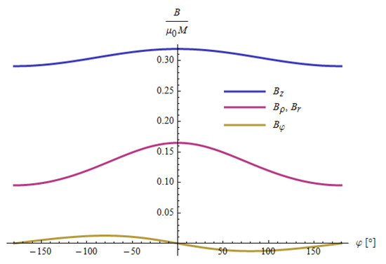
Figure 24.
Magnetic field components along an eccentric circle for = 2 mm, magnet diameter is 55 mm, magnet height is 15 mm (due to small , components and are nearly equal).
The most important conclusion from the above analysis is that the applied magnetic field along the measurement contour (where shown in Figure 21 was measured) may have a non-zero angular component, in addition to the fact that the axial component of the applied field is not constant along the contour. This leads to asymmetry in the peak visible in Figure 21. Apart from the asymmetric peak there is also visible a sinusoidal-like variation in the measured value, which probably originates from a small eccentricity in sample placement. In the simplified numerical computations, the presence of the component was simulated with a non-zero tilt angle of (Figure 18 and Figure 19).
From a theoretical point of view, the asymmetry in the peak can also be explained by magnetic charges attributed to both sides of the defect. For example, Zhao et al. [26] considered detection of stress corrosion, yet via the MFL method. In the case considered here, this reasoning is closer to the case of milled holes, but there is no corrosion stress. The influence of thermal or mechanical stresses has also been minimized by milling in a coolant environment. In the case described by us, there is a similar peak shape, but with a clear asymmetry, which causes a gap throughout the entire sample volume (Figure 21). Here, we are dealing neither with corrosion nor with stresses (waterjet); therefore, the nature of the phenomenon should be explained by the deviation of the magnetic flux angle from the Bz component (Figure 9) and the magnetic field density at the edge of the slot (Figure 8). Another possibility for describing the phenomenon was presented by Zatsepin and Shcherbinin [27]. In their view, this phenomenon is due to the demagnetizing field, which causes the appearance of free magnetic poles on the surfaces of the gap. They developed an analytical model for 2D point, infinite-line and semi-infinite-plane dipoles. The extension of the model to 3 dimensions is shown in [28].
3.6. Subsurface Defects
In the above considered cases, the drilled holes were only to simulate a defect that would be invisible under normal production conditions. The holes can represent air or nonmagnetic inclusions (polymers, rubbers, lubricants, copper, aluminum, etc.) that can enter the material during the manufacturing process, and are located on the surface or hidden just below it. Another type of defect is a change in the quality of the mixture from which the details are formed [20]. Detection of subsurface defects was indicated in [29], where a possibility for determining the localization and type (magnetic, nonmagnetic) of the inclusion based on magnetograms was shown, yet without a numerical analysis of the magnetic field around this type of defect.
In this subsection, it is assumed that the defect is a cylindrical inclusion of diameter D = 10 mm and height h = 2 mm, placed at a depth of d below the core surface. Figure 25 shows the effect of nonmagnetic inclusion located at various depths d = 0.5, 1, 2, 3, 4 mm. The shallow subsurface defects change the B field over the surface enough to be clearly registered. As the depth increases, the masking effect of the bulk material weakens the changes in the B field, and the defect can be undetectable.
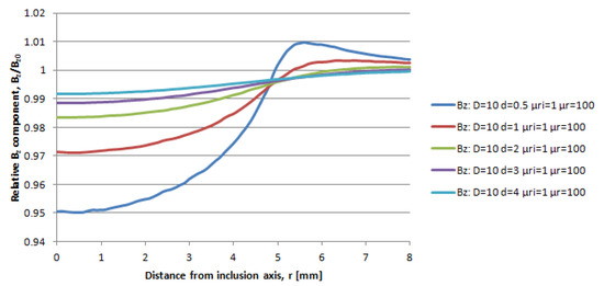
Figure 25.
Magnetic flux density distribution (z component) on the observation line over a cylindrical subsurface non-magnetic defect with a diameter D = 10 mm, height 2 mm, located at various depths d = 0.5, 1, 2, 3, 4 mm in SMC material of effective μr = 100.
Figure 26 shows the effect of the bulk effective permeability on the B field (z component) over a non-magnetic cylindrical defect with diameter D = 10 mm and a height of 2 mm, located at a depth of d = 1 mm below the core surface. For low effective permeability values (1 < μr ≤ 100), the defect is detectable via a Bz field analysis. When μr is large enough, the magnetic flux equalizes over the defect, hiding its presence.
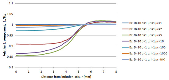
Figure 26.
Magnetic flux density distribution (z component) on the observation line over a cylindrical subsurface non-magnetic defect with a diameter D = 10 mm, height 2 mm, located at a depth of d = 1 mm in SMC material of various effective magnetic permeabilities μr.
The effect of the inclusion of magnetic permeability (μri) is shown in Figure 27. When μri is considerably less than μr, the Bz field is lower over the defect, with a peak over its edge shifted towards the bulk (blue, brown, magenta and cyan traces). When μri is considerably larger than μr, the z component of the B field is increased over the defect, and the peak occurs over the defect edge, with a shift towards the defect.
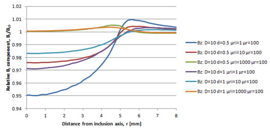
Figure 27.
Magnetic flux density distribution (z component) on the observation line over a cylindrical subsurface defect of various magnetic permeabilities and a diameter D = 10 mm, height 2 mm, located at depths d = 0.5 and 1 mm in SMC material of effective magnetic permeabilities μr.
An analysis of the above results, together with the magnetograms presented in [29], confirms that the considered method is able to detect shallow subsurface defects. Due to the masking effect of the bulk, detection becomes harder the higher the effective magnetic permeability of the bulk, and the deeper the defect is located.
4. Conclusions
The results of the experiments and numerical analysis indicate that the use of MagCam can be a valuable technique in NDT. In particular:
- The method allows for detection of both considered types of defects of different sizes on the surface and at different depths.
- Differences in surface sizes are more strongly reflected in the magnetic field images than defects of varying depths; therefore, it is easier to diagnose the surface size of the defect than its depth.
- The non-uniformity of the magnetic field and the possible presence of tangent components of the field have a great influence on the peak shapes over the defects; even small irregularities and small values of the tangential components cause asymmetry of the magnetic field distribution around the defect and the formation of larger field peaks near the defect. This should be considered as a positive effect by increasing the contrast of the flux outflow in the defect area.
- Shallow subsurface defects can be also detected, but the masking effect of magnetic bulk can hide the defect if it is sufficiently deep and small, or its magnetic properties are not sufficiently different from those of the bulk.
Further research will be focused on improving the measurement process, as well as on a more detailed analysis of the effects of various defects and other factors, such as non-homogeneity of the sample. An interesting direction could be a development of a hybrid method based on the presented approach and MFL. Moreover, it also seems reasonable to hybridize magnethography and active thermography, which, as a result of synergy, would be a powerful NDT method able to detect a wide range of defects. On the other hand, the presented method is quick in operation, and the resolution (geometrical and magnetic) offers the possibility for reliable detection of even small changes in the magnetic field due to possible defects.
Author Contributions
Conceptualization, A.J. and P.J.; methodology, A.J. and P.J.; software, P.J.; validation, A.J. and P.J.; formal analysis, P.J.; investigation, A.J.; resources, A.J.; data curation, A.J.; writing—original draft preparation, A.J. and P.J.; writing—review and editing, A.J. and P.J.; visualization, A.J. and P.J.; supervision, A.J.; project administration, A.J.; funding acquisition, A.J. Both authors have read and agreed to the published version of the manuscript.
Funding
Preliminary research was supported by the National Science Center of Poland, No. 2018/02/X/ST7/00410. The research was supported by the National Centre for Research and Development of Poland, grant, No. LIDER/11/0049/L-10/18/NCBR/2019.
Institutional Review Board Statement
Not applicable.
Informed Consent Statement
Not applicable.
Data Availability Statement
The data presented in this study are available on request from the corresponding author.
Conflicts of Interest
The authors declare no conflict of interest.
References
- Gholizadeh, S. A review of non-destructive testing methods of composite materials. Procedia Struct. Integr. 2016, 1, 50–57. [Google Scholar] [CrossRef]
- Seifi, M.; Gorelik, M.; Waller, J.; Hrabe, N.; Shamsaei, N.; Daniewicz, S.; Lewandowski, J.J. Progress towards metal additive manufacturing standardization to support qualification and certification. JOM 2017, 69, 439–455. [Google Scholar] [CrossRef]
- Hufenbach, W.; Böhm, R.; Thieme, M.; Tyczynski, T. Damage monitoring in pressure vessels and pipelines based on wireless sensor networks. Procedia Eng. 2011, 10, 340–345. [Google Scholar] [CrossRef]
- Jandejsek, I.; Jakubek, J.; Jakubek, M.; Prucha, P.; Krejci, F.; Soukup, P.; Zemlicka, J. X-ray inspection of composite materials for aircraft structures using detectors of Medipix type. J. Instrum. 2014, 9, C05062. [Google Scholar] [CrossRef]
- Fotsing, E.R.; Ross, A.; Ruiz, E. Characterization of surface defects on composite sandwich materials based on deflectrometry. NDT E Int. 2014, 62, 29–39. [Google Scholar] [CrossRef]
- Ramesh, P.; Lenin, N.C. High power density electrical machines for electric vehicles—Comprehensive review based on material technology. IEEE Trans. Magn. 2019, 55, 1–21. [Google Scholar] [CrossRef]
- Xu, W.; Duan, N.; Wang, S.; Guo, Y.; Zhu, J. Modeling and measurement of magnetic hysteresis of soft magnetic composite materials under different magnetizations. IEEE Trans. Ind. Electron. 2016, 64, 2459–2467. [Google Scholar] [CrossRef]
- Schoppa, A.; Delarbre, P. Soft magnetic powder composites and potential applications in modern electric machines and devices. IEEE Trans. Magn. 2014, 50, 1–4. [Google Scholar] [CrossRef]
- Wang, B.; Zhong, S.; Lee, T.L.; Fancey, K.S.; Mi, J. Non-destructive testing and evaluation of composite materials/structures: A state-of-the-art review. Adv. Mech. Eng. 2020, 12, 1–28. [Google Scholar] [CrossRef]
- Dwivedi, S.K.; Vishwakarma, M.; Soni, A. Advances and researches on non destructive testing: A review. Mater. Today Proc. 2018, 5, 3690–3698. [Google Scholar] [CrossRef]
- Jolly, M.R.; Prabhakar, A.; Sturzu, B.; Hollstein, K.; Singh, R.; Thomas, S.; Shaw, A. Review of non-destructive testing (NDT) techniques and their applicability to thick walled composites. Procedia CIRP 2015, 38, 129–136. [Google Scholar] [CrossRef]
- Dudzik, S.; Jakubas, A. Diagnostics of the Fe-based soft magnetics composites using active thermography. In Proceedings of the 2018 International Conference on Diagnostics in Electrical Engineering (Diagnostika), Předměstí, Czechia, 4–7 September 2018; pp. 1–4. [Google Scholar] [CrossRef]
- AbdAlla, A.N.; Faraj, M.A.; Samsuri, F.; Rifai, D.; Ali, K.; Al-Douri, Y. Challenges in improving the performance of eddy current testing. Meas. Control 2019, 52, 46–64. [Google Scholar] [CrossRef]
- Shi, Y.; Zhang, C.; Li, R.; Cai, M.; Jia, G. Theory and application of magnetic flux leakage pipeline detection. Sensors 2015, 15, 31036–31055. [Google Scholar] [CrossRef] [PubMed]
- Tessarolo, A.; Mezzarobba, M.; Menis, R. Modeling, analysis, and testing of a novel spoke-type interior permanent magnet motor with improved flux weakening capability. IEEE Trans. Magn. 2015, 51, 1–10. [Google Scholar] [CrossRef]
- Boero, G.; Demierre, M.; Popovic, R.S. Micro-Hall devices: Performance, technologies and applications. Sens. Actuators A 2003, 106, 314–320. [Google Scholar] [CrossRef]
- Smith, R.A.; Harrison, D.J. Hall sensor arrays for rapid large-area transient eddy current inspection. Insight-Non-Destr. Test. Cond. Monit. 2004, 46, 142–146. [Google Scholar] [CrossRef]
- Janousek, L.; Stubendekova, A.; Smetana, M. Novel insight into swept frequency eddy-current non-destructive evaluation of material defects. Measurement 2018, 116, 246–250. [Google Scholar] [CrossRef]
- Kosmas, K.; Sargentis, C.; Tsamakis, D.; Hristoforou, E. Non-destructive evaluation of magnetic metallic materials using Hall sensors. J. Mater. Process. Technol. 2005, 161, 359–362. [Google Scholar] [CrossRef]
- Jakubas, A. Diagnostics of the Fe-based composites using a magnetic field camera. In 2019 Progress in Applied Electrical Engineering (PAEE); IEEE: Piscataway, NJ, USA, 2019. [Google Scholar] [CrossRef]
- Jakubas, A.; Gębara, P.; Seme, S.; Gnatowski, A.; Chwastek, K. Magnetic Properties of SMC Cores Produced at a Low Compacting Temperature. Acta Phys. Pol. A 2017, 131, 1289–1293. [Google Scholar] [CrossRef]
- REMACOMP® C General Specification, Magnet-physik, Dr Steingroever GmbH. Available online: https://www.magnet-physik.de/upload/21278626-Remacomp-C-e-3153.pdf (accessed on 7 May 2021).
- Vervaeke, K. 6D magnetic field distribution measurements of permanent magnets with magnetic field camera scanner. In Proceedings of the 2015 5th International Electric Drives Production Conference (EDPC), Nuremberg, Germany, 15–16 September 2015; pp. 1–4. [Google Scholar] [CrossRef]
- Nishio, T.; Chen, Q.; Gillijns, W.; De Keyser, K.; Vervaeke, K.; Moshchalkov, V. Scanning Hall probe microscopy of vortex patterns in a superconducting microsquare. Phys. Rev. B 2008, 77, 012502. [Google Scholar] [CrossRef]
- Caciagli, A.; Baars, R.J.; Philipse, A.P.; Kuiper, B.W. Exact expression for the magnetic field of a finite cylinder with arbitrary uniform magnetization. J. Magn. Magn. Mater. 2018, 456, 423–432. [Google Scholar] [CrossRef]
- Zhao, B.; Yao, K.; Wu, L.; Li, X.; Wang, Y.S. Application of Metal Magnetic Memory Testing Technology to the Detection of Stress Corrosion Defect. Appl. Sci. 2020, 10, 7083. [Google Scholar] [CrossRef]
- Zatsepin, N.; Shcherbinin, V. Calculation of the magnetostatic field of surface defects. I. Field topography of defect models. Defektoskopiya 1966, 5, 50–59. [Google Scholar]
- Dutta, S.M.; Ghorbel, F.H.; Stanley, R.K. Dipole modeling of magnetic flux leakage. IEEE Trans. Magn. 2009, 45, 1959–1965. [Google Scholar] [CrossRef]
- Jakubas, A. Non-destructive study of the homogeneity of the structure of magnetically soft composites. Przeglad Elektrotech. 2021, 97, 136–139. [Google Scholar] [CrossRef]
Publisher’s Note: MDPI stays neutral with regard to jurisdictional claims in published maps and institutional affiliations. |
© 2021 by the authors. Licensee MDPI, Basel, Switzerland. This article is an open access article distributed under the terms and conditions of the Creative Commons Attribution (CC BY) license (https://creativecommons.org/licenses/by/4.0/).