Article

Analyzing Characteristics of Particulate Matter Pollution in Open-Pit Coal Mines: Implications for Green Mining

1
State Key Laboratory of Coal Resources and Safe Mining, China University of Mining and Technology, Xuzhou 221116, China
2
High-Tech Research Center for Open Pit Mines, China University of Mining and Technology, Xuzhou 221116, China
3
Haerwusu Open-Pit Coal Mine, China Shenhua Energy Co. Ltd., Ordos 017100, China
*
Authors to whom correspondence should be addressed.
Energies 2021, 14(9), 2680; https://doi.org/10.3390/en14092680
Submission received: 21 March 2021 / Revised: 29 April 2021 / Accepted: 1 May 2021 / Published: 7 May 2021
(This article belongs to the Special Issue Green Coal Mining Techniques 2021)

Abstract

:
The particulate pollution in the open-pit coal mines of China is particularly severe in winter. The aim of this study is to understand the pollution characteristics of particulate matter (PM) in winter and provide a basis for the prevention and control of particulate pollution. We took the problem of PM concentration at the bottom of the Haerwusu Open-pit Coal Mine (HOCM) as the research object. Dust monitoring equipment at two measurement points at different heights were positioned for continuous monitoring of the PM concentration. The data for three months were gathered. Statistical analyses were performed to analyze the variation characteristics of the PM and its relationship with meteorological factors. The results show that the average PM concentration in the study area is below the average daily limit of the China National Ambient Air Quality Standard (GB 3095-2012). However, the average concentration of PM10 exceeded the national limit in December. The order of PM concentration is observed as December > January > February. The correlation of PM is found to be positive with humidity and negative with wind speed. Temperature is found to be positively correlated with PM in December, while it is negative in January. At the same time, the temperature difference in December is negatively correlated with PM concentration. Under the combined action of multiple meteorological factors, the magnitude of the impact on the PM concentration at the bottom of the pit in winter is humidity > temperature > wind speed > temperature difference (inverse temperature intensity). In conclusion, PM2.5 is found to be more sensitive to environmental factors. The results of this study are particularly useful to progress in green mining.

1. Introduction

The mining industry has faced severe environmental challenges in its supply chain due to high pollution and damage to the ecosystem resulting from mineral extraction activities [1,2]. These challenges destroy the natural environment around the mining area, putting the entire ecosystem, humans, wildlife, and plants at risk. They are also regarded as the initiating point for a mining project to be unsustainable [3,4].
Air pollution during mining operations is one of the most common environmental issues [5]. Both underground and surface mining operations exacerbate it due to the generation of large amounts of dust [6]. The dust accumulated in various locations in and around the mining area results in substantial degradation of vegetation cover and the diversity of plants and animals. In addition to reducing crop production, it can also pollute the downstream areas [7]. An excessive amount of dust is harmful to the atmosphere because it reduces atmospheric water retention while raising temperature [8]. Dust pollution also brings a series of problems to the development of the mine. The issues, which affect production efficiency, include poor visibility of the working environment and potential health and safety risks. Managing air pollution by controlling dust emissions is becoming more challenging with increased production capacity [9].
At present, coal remains China’s primary energy source, fueling the country’s economic growth and rendering China the world’s largest coal producer [10]. In the near future, the demand for coal is likely to continue, which, in turn, will increase the share of coal production from open-pit mines [11]. Even though the accelerated development of coal can stimulate economic growth, it impedes sustainable development due to its social problems and ecological deterioration [12]. The exhaust emissions from coal mining, primarily smoke, dust, and other gases, cause varying levels of damage to the atmospheric environment, making the industry the fifth-largest emitter of industrial pollution in the country [10]. Evidence suggests that PM contributes significantly to air pollution, especially during the winter [13]. In China, more than 90% of the coal production from open-pit mines originates in extremely cold and arid climate zones. The operational characteristics of open-pit coal mines are stripping in spring and summer and exploitation in autumn and winter. These operations cause significant dust pollution, which is challenging to manage with traditional water spraying. Due to the slow speed and low frequency of wind in winter, mining zones are prone to long-term static weather. Dust is usually not released into the atmosphere through the air but mainly concentrated at the bottom of the pit. Moreover, several meteorological factors (e.g., wet and foggy conditions and reduced wind speed) inhibit the spread of dust and thus intensify its deposition and accumulation. In this situation, the problem of PM concentration at the bottom of the open-pit mine is prominent, causing severe environmental pollution, reducing atmospheric visibility, and having a detrimental impact on human health [14,15,16]. As a result, dust pollution in mines is considered a major environmental, social, and technical issue. Many studies have advocated the need for its monitoring, evaluation, and control measures in order to make adequate progress towards the success of green mining [1,17,18,19,20]. Therefore, it is necessary to understand the characteristics of PM pollution in open-pit mines and analyze the influence of meteorological factors on their concentration.
This research was conducted to explore the distribution of PM pollution and the influence of meteorological conditions on its concentration in open-pit coal mines located in cold and arid climate regions by taking one of the largest coal mines in China, Haerwusu Open-pit Coal Mine (HOCM), as the research site for the case study. To achieve this goal, the concentration of three different fractions of PM: TSP, PM10, and PM2.5, as well as metrological factors including temperature, humidity, wind speed, and wind direction, were measured over the period of three months, i.e., from December to February. The first objective was to analyze the level and variation of PM characteristics in the mine. The second objective was to discover the correlation between PM pollutants. Finally, the influence of meteorological factors on PM concentration was investigated. To pursue the purpose of the investigation, statistical analyses, including descriptive analysis, Pearson’s correlation coefficient, principal component analysis (PCA), and regression modeling, were performed using SPSS 24 statistical software package. The study results serve as the basis and theoretical reference for breaking through the bottleneck of dust prevention and control in winter, which most open-pit coal mines in China face in their efforts to progress into green mining.

2. Literature Review

In terms of air pollution, it is reported that dust emission from surface mining is more than those from underground mining [21]. A large amount of particulate matter (PM) is produced in all stages of open-pit operations, such as exploration, stripping, drilling, blasting, exploitation, transportation, crushing, and disposal [22,23]. Therefore, open-pit mining is known to be one of the main sources of particulate matter (PM) of different sizes [17,24]. Among other sources of pollution in mining regions, PM pollutants that cause air quality degradation and lead to adverse effects on human health are a cause of serious concerns when their levels in the air are high [25,26,27]. The size of PM is an important factor in determining health risks. PMs with aerodynamic diameters of up to 10 m, 2.5 m, and 1 m pose a major risk to human health [28]. Particles equal to and greater than 30 μm (known as total suspended particulate (TSP) matter) are very coarse particles that settle very close to the point of emission [29]. Particles between 30 and 10 μm in size remain suspended in the air for a limited time, and they get trapped in the nostrils or mouth and are swallowed [30]. PMs with aerodynamic diameter <10 µm (PM10) are more likely to be inhaled through the respiratory tract [31,32]. Particles <2.5 μm (PM 2.5) and fine particles up to 1 μm (PM1) are inhaled deep into the lungs [30,33,34]. Although high concentrations of PM pose serious health risks, it is also evident that prolonged exposure even to low levels of PMs in the air leads to increased hospitalization and death [35]. Therefore, the PM pollution in open-pit mines has become a widespread concern due to its numerous consequences [36]. It has piqued the interest of researchers all over the world, who are now delving deeper into analyzing it from different perspectives [37,38]. For instance, Yadav and Jain [39] investigated the mass and concentration of PMs under dry and wet weather in the mining and non-mining areas of Jharkhand, India. The concentration of PM10 and PM2.5 was maximum in mining areas, exceeding the limits of Air Quality Standards in India and the World Health Organization during dry weather, but decreased significantly due to precipitation during the wet weather. Wanjun and Qingxiang [40] analyzed dust distribution in a Chinese open-pit coal mine and found that PM concentration is nearly the same throughout the mine, but its concentration is very high around the equipment working area, i.e., 426 μg/m3. Quite recently, Li, et al. [36] monitored dust in the Pingshuo mining area, China, to reveal concentration change during a 24-h cycle. Average PM concentrations were determined to be approximately 60 μg/m3, 114 μg/m3, and 250 μg/m3 for PM2.5, PM10, and TSP, respectively. Research on emissions structure and volume of gas and PM from mining and quarrying in EU countries reveals that the UK and Germany are the largest emitters of PM2.5, followed by Poland, France, and Sweden. Conversely, in terms of PM10, the highest emissions were recorded in Germany, UK, France, and Poland, respectively [41]. In Australia, PM levels were measured in mining and non-mining communities in Queensland and New South Wales during 2008–2018, indicating a significant rise in PM and other pollutants over the timeframe studied with the increase in coal production, where coal mines accounted for 42.1% and 19.5% of the national PM10 and PM2.5 air emissions, respectively [5].
Meteorological variables are well recognized in the intensifying air pollutants, which play a crucial role in the dispersion of PM in the air [28,42]. Compared with other seasons, weather conditions in winter are favorable for dust deposition and accumulation due to wet and foggy conditions with low wind speed preventing particulate dispersion [43,44]. It is believed that although meteorological factors affect PM concentration, their effects differ depending on the season and location [45]. Researchers use many analysis and prediction methods to investigate the problem of dust concentration and identify its relationship with meteorological factors [46]. In previous literature, it is found that statistical analysis is an effective means to study the pollution level and influencing factors of atmospheric PM [47,48,49]. Huertas, et al. [50] studied PM concentration at several locations in the open-pit coal mining region of northern Colombia under the influence of meteorological factors using multiple regression. They found that environments drier than 54% lead to pollution. In comparison, humidity levels greater than 70% maintain safe air quality conditions in the area, and there is a higher relationship between meteorological variables and PM concentrations. Oguntoke, et al. [51] conducted a multivariate analysis to quantify the influence of meteorological parameters on the emission of mine dust in Witwatersrand, South Africa, which showed that the deposition rates of dust were different in different seasons, with the highest deposition level and frequency in spring, a negative correlation between humidity and dust, and a positive correlation between wind speed and dust. In an Iranian open-cast copper mine, a study finds that PM10 and TSP concentrations are lowest in autumn and winter, respectively, while both have the highest concentration in summer [35]. A case analysis of dust and noise control in a Serbian copper mine that took into account meteorological conditions revealed that the distribution of PM10 concentration has a significant impact around the open pits [52].
There have been many studies that applied statistical methods to assess the relationship between PM concentration and meteorological conditions in urban areas of many countries, including China [53], Korea [54], and European countries [55]. However, there have been quite a few studies in the literature analyzing these aspects in open-pit mines [28]. It is therefore imperative to assess the correlation between PMs and the influence of meteorological factors on the concentration of PMs in open-pit mines, as this research gap is identified in the literature [17,36,54]. Several earlier studies have some limitations and only apply to certain special cases, meaning they cannot be applied universally [36]. Since PM concentrations in different seasons and locations are different, their relationship with meteorological variables will also be different. Therefore, site-specific analyses are required to compare the results and to formulate and subsequently implement control strategies [17,29,56].

3. Materials and Methods

3.1. Overview of the Research Area

HOCM is located in Ordos, Inner Mongolia, China. It is one of the largest open-pit coal mines in China, with an annual output of more than 30 Mt. The mining region has a typically arid continental climate with significant temperature differences between summer and winter. The average temperature in winter ranges from −11 °C to −1 °C, the lowest temperature reaches about −30 °C, and there are many (around 4–6) gale periods. The frost period lasts approximately 150 days, from early November to early April. In spring and autumn, the region is windy and dry, with an average temperature between −10 °C and 3 °C. The weather fluctuates drastically during the day, with large variations in morning and evening temperature. Summer is hot, with an average temperature of 10 °C to 23 °C. Rainwater is concentrated in July, August, and September, accounting for about 65% of the annual precipitation. The annual precipitation is about 400 mm, and the evaporation is five times the precipitation. Drought and wind contribute to the emergence of sand and dust storms, with the average annual sandy day being 32.8 days and the average annual sandstorm day being 15.2 days. The land is barren and unused, with relatively low natural vegetation, no farmland and woodland, and a fragile ecological environment.

3.2. Monitoring Instruments

This research required continuous and real-time monitoring of the PMs and metrological conditions, so the equipment used had to be capable of continuous detection, moisture resistance, and low-temperature resistance.
The equipment used was the RS-ZSYC-9S-4G multi-parameter monitoring device, manufactured by Shandong Renke Measurement and Control Technology Co., Ltd. (Jinan, China). The device was equipped with various sensors to measure the temperature, humidity, wind speed, wind direction, and PM. Table 1 shows the measurement range, resolution, and precision of the device.

3.3. Layout of Measuring Points

The device was installed according to the existing operating area of the mine. Two monitoring points were selected in the mine, as shown in Figure 1. The vertical height between the two measurement points was about 180 m, and the horizontal distance was about 400 m. Monitoring point 1 was positioned on the earth’s surface, and as seen in Figure 1b, the position of the device was fixed. Monitoring point 2 was at the bottom of the pit, and the equipment could dynamically move with the work progress, as shown in Figure 1c. The device uploaded the data to the cloud server in real-time through the 4G network. The frequency of data collection in the experiment was set to be a five-minute interval, which recorded 12 data points in an hour and 288 in a day. The data was recorded for a total of three months, providing a total of 26,000 collected data points.

3.4. Data Analysis

The collected data was managed in SPSS version 24 for performing statistical analyses, described below.
It is well recognized that large datasets often contain outliers due to recording errors or data management errors, which may have a significant impact on the analysis results. Therefore, it is very important to detect values that are statistically significantly different from the observed values to avoid misspecification in the evaluation, which could result in a high cost for its improvement [57,58]. To detect the outliers, the most applied classical rule based on the z-score of the observations was used, i.e., the observational value minus the mean, divided by the standard deviation [59,60]. Before performing analysis between variables whose units are different from each other, it is necessary to first standardize the data so that it is internally consistent and representable in a uniform structure and format. In this study, the Z standardization method provided by SPSS was used.
The descriptive analyses were performed to characterize the data of PM concentration. Pearson’s correlation coefficient was used to investigate the correlation between TSP, PM10, and PM2.5 at a significance level of p < 0.01. Pearson’s correlation coefficient corresponds to a standardized covariance matrix, which is not affected by the scale of each variable and can more objectively reflect the correlation degree of the relationship between multiple variables. Regression coefficients between PM10 and TSP were calculated using curve estimation. In order to analyze the dependence of PM concentration on meteorological elements more intuitively, PCA was used, which transforms several potentially correlated variables into a smaller number of variables, called principal components. The PCA method is to sequentially find a set of mutually orthogonal coordinate axes from the original space. The choice of the new coordinate axis is closely related to the data itself. Among them, the first new coordinate axis selection is the direction with the largest variance in the original data, the second new coordinate axis selection is the plane orthogonal to the first coordinate axis that maximizes the variance, and the third axis is the largest variance in the plane orthogonal to the first and second axes. By analogy, such coordinate axes can be obtained. With the new coordinate axis obtained in this way, most of the variance is contained in the first k coordinate axes, and the variance contained in the latter coordinate axis is almost zero. Therefore, the number of principal components is less than or equal to the number of original variables, giving a linear combination of the original data. The variance was estimated for each independent variable (meteorological elements). This method generates the principal components by identifying the variables with the highest factor loadings in relation to the component data. As a result, the new principal components are a linear combination of explanatory variables (meteorological elements) that have the greatest influence on the components and the PM concentration (dependent variable). Kaiser-Meyer-Olkin (KMO) test and Bartlett’s were performed to check for sampling adequacy and sphericity, respectively. KMO is an index used to compare the simple correlation coefficient and partial correlation coefficient between variables. The closer its value is to 1, the more suitable the variable is for factor analysis. The statistics of the Bartlett sphere test are obtained according to the determinant of the correlation coefficient matrix. If the significance test is passed, it is suitable for analysis. To analyze the rate of contribution of each meteorological factor to PM concentration, regression models were developed. For this, multiple regression analysis was performed that analyzed the relationships between PM concentration and meteorological factors. It established the quantitative relationship between mathematical models among variables and effectively determined the significant variables that affect the dependent variable. In the last step, the relative importance of multiple independent variables to the model was analyzed using the relative weight method.

4. Results and Analysis

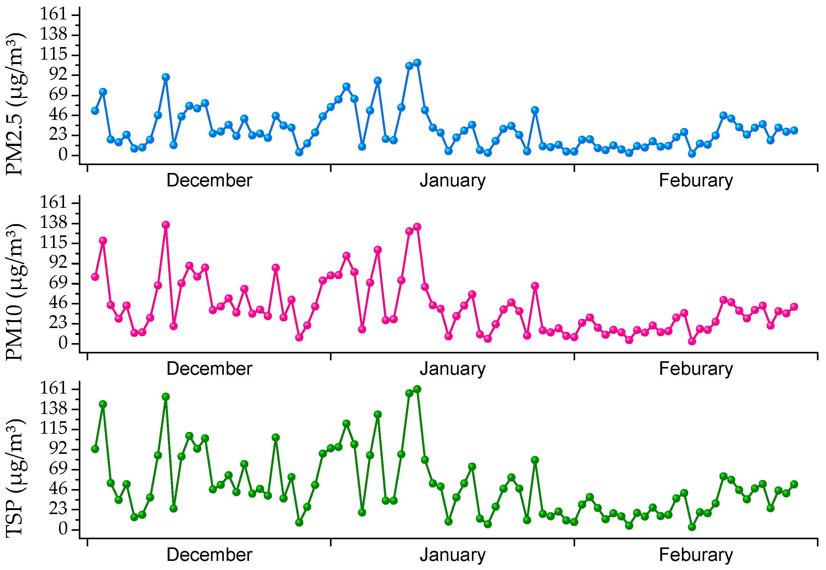
4.1. Monitoring Results

The basic statistics of the monitoring results are shown in Table 2. The statistical variables include temperature at point 1 (T1), humidity at point 1 (R1), wind speed at point 1 (S1), the temperature at point 2 (T2), humidity at point 2 (R2), wind speed at point 2 (S2), and TSP, PM10, PM2.5 at point 2.

4.2. Characteristics of PM Concentration

The statistics of TSP, PM10, and PM2.5 concentrations measured in the pit bottom are shown in Table 3, which shows that the order of pollution in each month is as of December > January > February. The results are compared with the National Ambient Air Quality Standards (GB3095-2012) in China. The national requirements of the average concentration limit of PM are shown in Table 4. According to the observations, the level of PM pollution in winter was lower than the daily limit, except that the PM10 in December exceeded the first-level standard limits. For average annual limits, TSP was below the national limits. However, both the PM10 and PM2.5 were above the first-level national limits. Only PM10 was relatively below the limit in February. Although the average concentrations of TSP, PM10, and PM2.5 vary in different months, the overall trend is consistent, indicating that there may be a correlation between them.
Figure 2 shows the changes in PM concentrations with time. It helps to analyze the relationship of TSP, PM10, and PM2.5 with time. The changes of TSP, PM10, and PM2.5 show significant consistency. In Figure 3, the proportion of PM concentration with time is shown, representing the amount of PM10 and PM2.5 in TSP. The larger the ratio, the higher the concentration of PM10 and PM2.5 in TSP. Notably, the particle size of PM2.5 is relatively small, making it easy to adsorb toxic substances such as heavy metals, which is harmful to the ecological environment and the human body. It can be observed that the proportion of PM10 in TSP is more than 80% in the HOCM with relatively minor variations in the proportion ratio. The proportion of PM2.5 in TSP is greater than 40% but less than 80%. However, the proportional ratio varies over time. In contrast, PM2.5 accounts for a large proportion in PM10, ranging from 50% to 90%, with quite significant fluctuations in its proportion. Since the ratio of PM2.5/TSP is different from that of PM10/TSP, PM2.5 may be more sensitive to environmental factors. Accordingly, the PM in winter is mainly fine, leading to poor air quality.
Through the above analysis, it can be determined that there is a certain correlation between TSP, PM10, and PM2.5. Therefore, a correlation analysis was performed between them, and the results are shown in Table 5. According to the two-tail test, there is a significant correlation between them. The correlation coefficients between the particulates are more than 0.9. To further quantify the relationship between PM concentration, regression analysis was performed. The regression analysis of the PM10 and TSP found that the power function best fitted, with the degree of fit of 0.985, and passed the significance test. The specific coefficients are shown in Table 6.
The regression equation between PM10 and TSP can be written as:
ln ( PM 10 ) = ln ( 0.895 ) + 0.981   ln ( TSP )
In general form:
PM 10 = 0.895 ×   TSP 0.981
Similarly, the regression analysis between PM2.5 and TSP shows that the power function was the best fit with the values of 0.959 and 0.966, respectively. The regression equation of PM2.5 and TSP is:
PM 2.5 = 1.047 ×   TSP 0.855
The regression equation of PM2.5 and PM10 is:
PM 2.5 = 1.168 ×   PM 10 0.868

4.3. Influence of Meteorological Factors on the PM Concentration

4.3.1. Relationship between PM Concentration and Relative Humidity

Using the field measurement data, the monthly average relative humidity data of the two measurement points in the study area was obtained, as shown in Figure 4. It can be seen that the relative humidity of HOCM is the lowest in January and the highest in February. The relative humidity in different locations in each month is relatively close. The results of the correlation analysis of relative humidity and PM are shown in Table 7. There is a positive correlation at different locations in different months. In addition, PM2.5 has a higher correlation coefficient than TSP, PM10, and relative humidity.

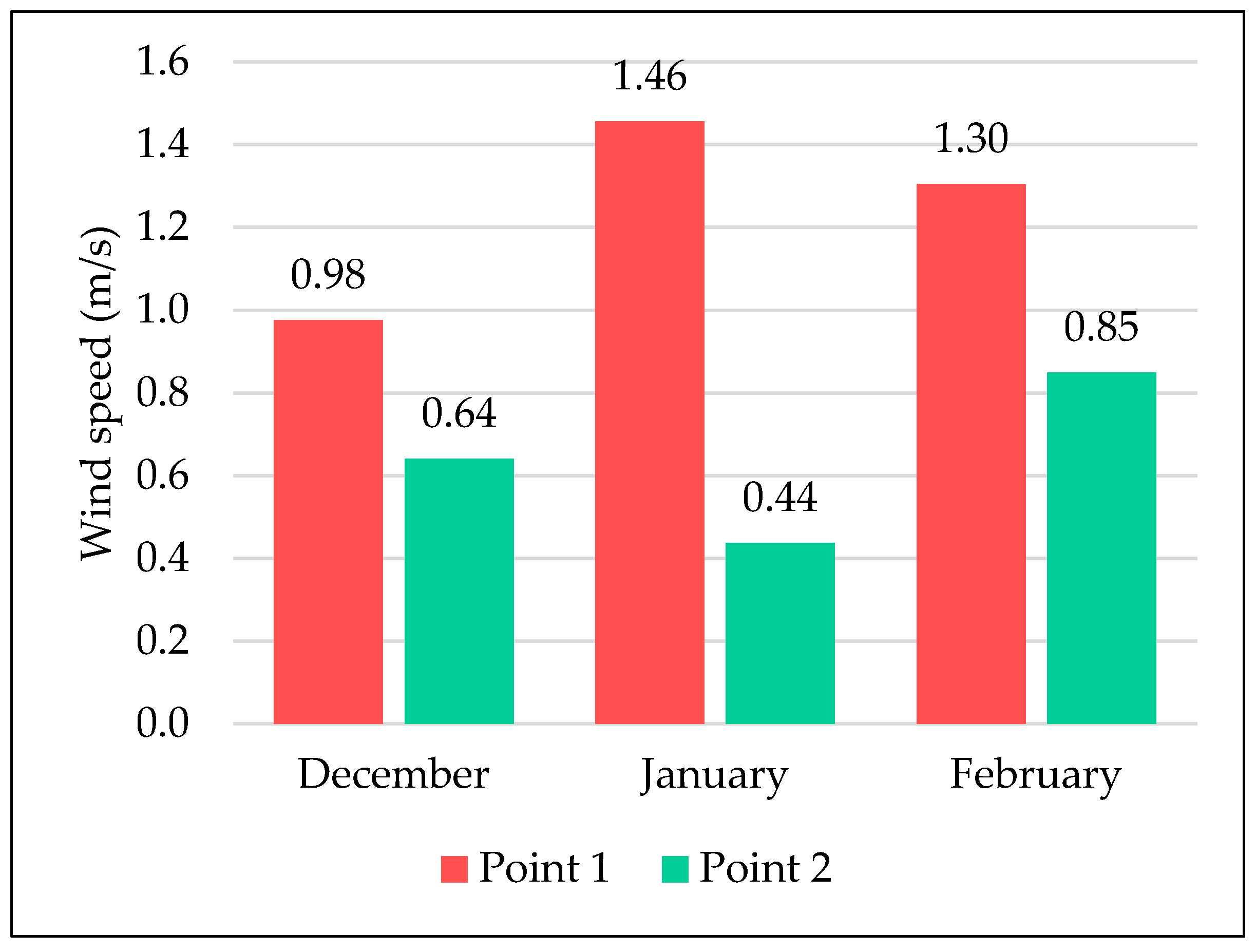
4.3.2. Relationship between PM Concentration and Wind Speed

The average wind speed of each month is shown in Figure 5. The average wind speed at different levels of HOCM in each month is significantly different, which is lower at the bottom of the pit than the surface every month. Wind speed less than 1 m/s indicates that the topography of the depression significantly changes the wind flow field, making the wind speed at the bottom of the pit far less, especially in winter. The results of the correlation analysis are shown in Table 8. Results indicate that in winter, there is a negative correlation. It is clear that the smaller the particle size of the PM, the higher the correlation coefficient of wind speed.

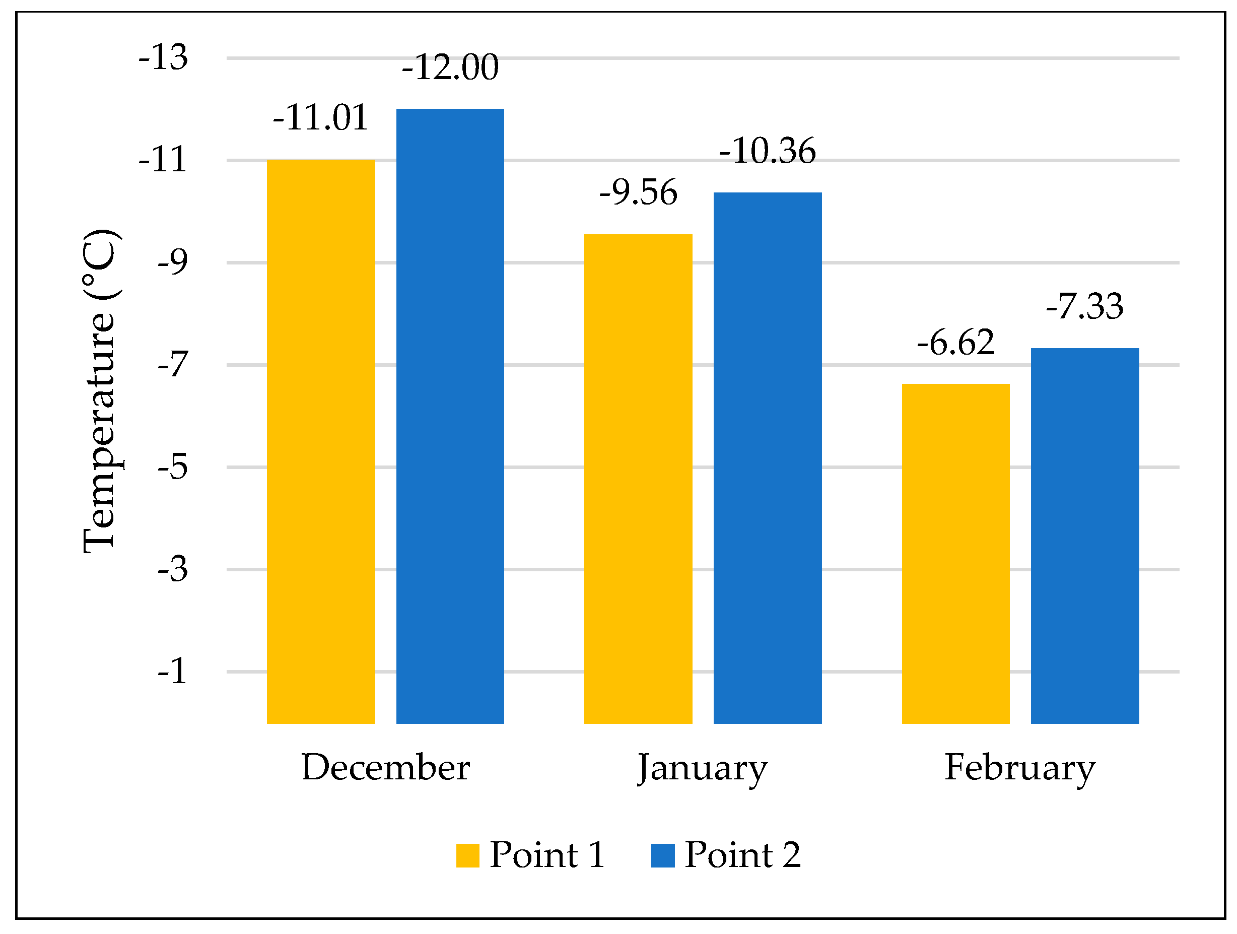
4.3.3. Relationship between PM and Temperature

The average temperature of each month at different locations is shown in Figure 6. The temperature in HOCM is the lowest in December, followed by January and February. The results of the correlation analysis of the temperature data and the PM concentration at the corresponding time are shown in Table 9. The influence of temperature varies in different months. Although the data in February month passed the significance test, its correlation coefficient is small, so the temperature in this month has a little effect on the PM concentration. The temperature in December is positively correlated with PM concentration, and January temperature is negatively correlated with PM concentration.

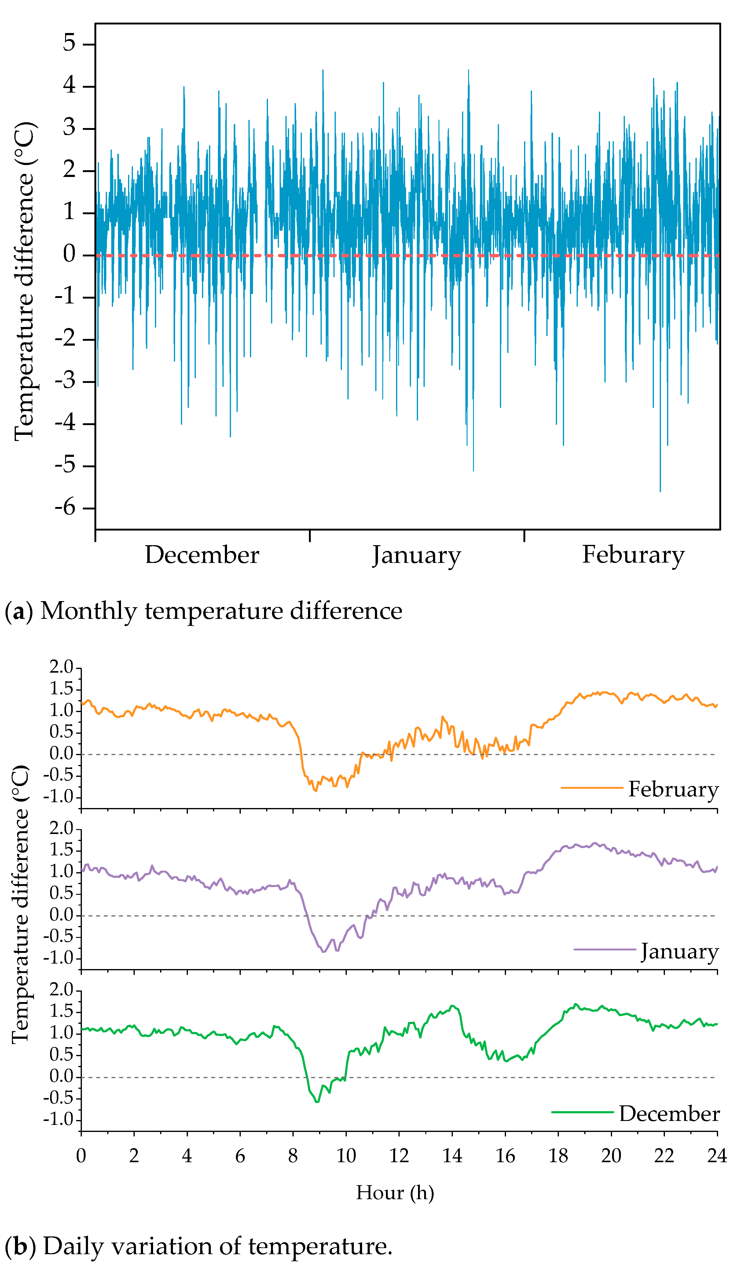
4.3.4. Relationship between PM Concentration and Temperature Difference

The average temperature at the bottom of the pit is less than the average temperature at the surface, indicating that there is an inversion phenomenon in the open-pit coal mine in winter. It is illustrated in Figure 6. Air inversion could block vertical air convection and reduce the vertical diffusion of pollutants. Therefore, it is necessary to analyze the characteristics of winter inversion. It can be achieved by subtracting the average of the pit bottom at the corresponding time from the average at the surface. If the value is positive, there is an inverse temperature phenomenon. The temperature difference between the two levels in winter is shown in Figure 7a. The temperature difference between the two measuring points fluctuates between 0–2 °C in winter. The part with a positive temperature difference is much larger than the region with a negative temperature difference, indicating a long-term temperature inversion phenomenon in open-pit coal mines in winter. To further analyze the time when inversion occurs, the daily variation characteristics of temperature in each month were analyzed, as shown in Figure 7b. According to results, the characteristics of temperature inversion of each month have a more consistent change pattern. There are two valleys, corresponding to the time at approximately 9:00 and 16:00 every day. The period of the inversion phenomenon dissipation is around 8:00–11:00 every day. Correlation analysis was conducted between the temperature difference data and the PM concentration at the same time. According to the results shown in Table 10, there is a negative correlation between the temperature difference and the PM concentration in December. In January and February, there is almost no correlation between the temperature difference and the PM concentration.
The PCA was performed to better reflect the relationship between the meteorological factors and the PM concentration. First, the variables with significant multicollinearity need to be eliminated to avoid analysis errors. The multicollinearity is an approximately linear relationship between independent variables; that is, an independent variable can be approximately described by the linear function of other independent variables. The linear regression identified the multicollinearity in the temperature at measuring point 1 and the humidity at measuring points. Therefore, after eliminating them, a total of eight variables were finally selected for analysis. They include the wind speed at the point 1 (S1), the relative humidity at the point 2 (R2), the temperature at the point 2 (T2), the wind speed at the point 2 (S2), the temperature difference (W), TSP, PM10, and PM2.5.
KMO and Bartlett sphericity tests were performed on the data, as shown in Table 11. The KMO value of 0.797 was obtained. Both the tests are statistically significant (p < 0.01). It shows that there are significant differences between the correlation coefficient matrix and the unit matrix. Through PCA, a total of three principal components were extracted. The cumulative variance contribution rate is 76.143%, indicating that there is no significant information loss of the original variable. After the rotation, the individual variance contribution rate of the three components was changed. However, their cumulative variance contribution rate did not change. It implies that it does not affect the commonality of the original variables. Therefore, principal components are considered to be suitable (Table 12). As shown in Figure 8, principal component 1 includes R2, TSP, PM10, and PM2.5, principal component 2 includes S1 and S2, while principal component 3 includes T2 and W. It further shows that the correlation between humidity and PM concentration is the most significant.

4.4. Multiple Regression Model of PM Concentration and Meteorological Factors

From the analysis of the influence of metrological factors on PM concentration, it can be observed that many factors affect the PM concentration at the bottom of the pit. If a single factor is used to analyze the various characteristics of the PM concentration, a one-sided error may occur. Therefore, multiple stepwise regression analyses were also performed. Through this method, the meteorological factors that affect PM concentration can be effectively determined. The regression between dependent variables (TSP, PM10, and PM2.5) and independent variables (T2, R2, S2, S1, and W) were analyzed to construct multiple regression models. The specific results are shown in Table 13. It can be found that the meteorological factors that significantly affect the PM concentration include humidity, temperature, wind speed, and temperature difference. The fitting degree of the regression model is PM2.5 > TSP > PM10.
To calculate the relative importance of independent variables, the relative weight method was used. It can help interpret the explanatory rate of independent variables to model variance. To be more specific, the contribution of metrological factors to the PM concentration can be quantitatively evaluated. Durbin-Watson test was used to detect the presence of autocorrelation of residuals in a regression analysis. The results, shown in Figure 9, can be interpreted as the higher the explanatory rate of model variance, the greater the contribution of independent variables to the PM concentration. Taking PM10 as an example, the interpretation rates of independent variables R2, T2, S2, and W for R2 (0.552) are 76.1%, 23.0%, 0.5%, and 0.4%, respectively. PM2.5 and TSP also show the same trend. Therefore, the order of influence of meteorological factors on the PM concentration is humidity > temperature > wind speed > temperature difference. The cumulative interpretation rate of humidity and temperature is about 99%, indicating that the PM concentration is mainly affected by humidity and temperature.

5. Discussion

The monitoring and analysis of the PM at the bottom of the pit of the HOCM in winter is of great importance to understand the air pollution caused by mining in the severe cold and arid area. The results indicate that PM pollution in winter exceeded the permissible annual average concentration limits in the country, especially in December and January. Since HOCM is located in an ecologically fragile area, permissible limits may be further improved because the pollution of HOCM is the most serious in winter. Although this problem is considered high, the literature reports even PM concentration in the mining areas. In Thailand, PM10 concentration in winter was found to be high due to cool and dry weather [61].
According to the analysis of PM in winter, there is a significant correlation between TSP, PM10, and PM2.5. The relationship between them can be fitted by a power function. These results are consistent with the conclusions of Wanjun and Qingxiang [40]. They reported that in HOCM, the concentration of PM10 and PM2.5 changes together. Therefore, the concentration of two particles (i.e., PM2.5 and TSP) can be estimated from the concentration of a single particle (i.e., PM10), which can significantly reduce the particle sensor in the mine so as to improve the level and cost of management of monitoring equipment. The influence of humidity in winter on PM concentration is more prominent, showing a positive correlation, indicating that the greater the winter humidity, the easier it is to cause serious pollution of the pit bottom. These results are in line with the results of Liao, et al. [62]. The main reason is that the relative humidity in winter is low. The moisture content in the air is not big enough to increase the particle size to a large amount of sedimentation but could result in haze phenomenon and increase air pollution. The negative correlation between wind speed and PM concentration indicates that wind speed can dilute PM concentration, which is consistent with the conclusions of Galindo, et al. [63]. According to a study of PM characterization in an Indian mining region, the impact of high wind speed leads to the decrease of PM2.5 and PM1, while this pattern does not exist in the case of PM10 [64]. The effect of temperature on the PM concentration in different months has two sides. At low temperatures, the ground turbulence intensity is weak, and the particulates are easy to gather. The increase in temperature can increase the ground turbulence intensity and reduce the particle concentration. The temperature difference is negatively correlated with PM in December. The main reason is the extremely low temperature at night. There is no wind, the vertical and horizontal diffusion of dust is hindered, and the PM is concentrated in the mining area. Although the temperature inversion intensity at the bottom of the pit is weakened in the daytime, the turbulence is strengthened. The dust in the mining area flows to the bottom of the pit, and the PM concentration at the bottom of the pit increases. Hence, the influence of meteorological factors on small particles is more obvious.
Through regression analysis and relative weighting, it can be found that considering many meteorological factors at the same time, the influence of humidity on PM concentration is more significant, followed by temperature, wind speed, and temperature difference. These findings are almost consistent with the findings of Qi, et al. [65], who reported that PM concentration in the same mine is influenced by humidity, temperature ≈ noise level, wind speed, and wind direction. From the value of R2 of the model, it is noticeable that the smaller the particle size of the PM, the higher the fit of the equation, indicating that the particle size is more sensitive to meteorological factors. In addition, the fitting degree of PM10 and TSP is quite close, again proving that most of the TSP at the bottom of the pit is PM10.
Continuous monitoring instruments were used in this research to monitor PM concentration and meteorological factors in winter. However, in the actual monitoring process, the equipment at the pit bottom must be movable in real-time. Since the equipment was not fixed at the pit bottom, the effect of wind direction on the PM concentration is not discussed. Furthermore, because the monitoring equipment is expensive, only two devices were installed, resulting in the limited disclosure of pollution characteristics to a certain extent. It should also be noted that there is almost no natural wind at the pit bottom in winter, and the distribution of PM was uniform. Therefore, research results can provide a reference for understanding PM pollution under different meteorological conditions. Future research should consider more observation points and longer period data to compare the relationship between PM pollution and meteorological factors. The influence of some other meteorological factors can also be considered. Of course, the ultimate goal of studying the relationship between dust concentration and meteorological factors is to reduce dust pollution. Therefore, future studies should investigate how to use meteorological factors and operational parameters of mine to obtain the criterion of the pollution degree, so as to provide a basis for optimizing the operation parameters of the mine and advancing the practice of green mining.

6. Conclusions

Open-pit operations are inherently associated with dust generation, which gives rise to significant concerns in the practice of green mining by impacting the production, productivity, health, and safety of miners. Dust issues in open-pit mines have been widely studied. However, little attention has been paid to monitoring dust generation and dispersion in different seasons to analyze the characteristics of PM pollution. This study is intended to understand the PM concentrations, thus increasing confidence with respect to control the air pollution caused by dust in open-pit operations. The main contribution of this study is to estimate PM concentration in relation to different meteorological factors, suggesting that the monitoring and control of PM must be optimized. It is concluded that the PM concentration exceeded the first and second level limits of national ambient air quality. The order of the average PM concentration is December > January > February. In winter, PM10/TSP value is stable at around 80%, and PM2.5/TSP and PM2.5/PM10 values fluctuate significantly. As a whole, they are at a high level, indicating that the winter is dominated by small particle-sized particulate pollution and poor air quality. In December, PM concentration is found positively correlated with humidity and temperature while negatively with wind speed. In January, analysis shows that PM concentration positively correlates with humidity and negative with wind speed. Temperature is found to be positively correlated with PM in December, while it is negative in January. The temperature difference (inverse temperature intensity) in December is negatively correlated with PM concentration. It should be noted that temperature within a certain range can promote dust diffusion, but the lower temperature will increase pollution. Considering the combined influence of multiple meteorological factors, the order of influence on the PM concentration in winter is humidity> temperature> wind speed> temperature difference. The reduction of dust and lessen the impact of PM pollution has become increasingly prominent in the wake of cleaner and sustainable mineral production. Therefore, it is suggested that green mining should be implemented and engineering solutions for dust control be developed and applied.

Author Contributions

Conceptualization, H.L. and W.Z.; methodology, I.M.J. and Z.W.; investigation, H.L. and Z.W.; resources, W.Z.; writing—original draft preparation, I.M.J. and Z.W.; writing—review and editing, I.M.J.; supervision, W.Z.; funding acquisition, W.Z. All authors have read and agreed to the published version of the manuscript.

Funding

This study was supported by the Independent Research Project of State Key Laboratory of Coal Resources and Safe Mining, China University of Mining and Technology (SKLCRSM18X001).

Institutional Review Board Statement

Not applicable.

Informed Consent Statement

Not applicable.

Data Availability Statement

Not applicable.

Acknowledgments

We would like to thank Harwusu open-pit coal mine for providing a research base for this paper. We also thank the relevant technicians on-site for maintaining the equipment.

Conflicts of Interest

The authors declare no conflict of interest.

References

  1. Jiskani, I.M.; Cai, Q.; Zhou, W.; Shah, S.A.A. Green and climate-smart mining: A framework to analyze open-pit mines for cleaner mineral production. Resour. Policy 2021, 71, 102007. [Google Scholar] [CrossRef]
  2. Brodny, J.; Tutak, M. Can the current environmental tax rate promote green technology innovation?—Evidence from China’s resource-based industries. J. Clean. Prod. 2021, 278, 123443. [Google Scholar] [CrossRef]
  3. Jiskani, I.M.; Cai, Q.; Zhou, W.; Lu, X. Assessment of risks impeding sustainable mining in Pakistan using fuzzy synthetic evaluation. Resour. Policy 2020, 69, 101820. [Google Scholar] [CrossRef]
  4. Jiskani, I.M.; Cai, Q.; Zhou, W.; Chang, Z.; Chalgri, S.R.; Manda, E.; Lu, X. Distinctive model of mine safety for sustainable mining in Pakistan. Min. Metall. Explor. 2020, 37, 1023–1037. [Google Scholar] [CrossRef]
  5. Hendryx, M.; Islam, M.S.; Dong, G.-H.; Paul, G. Air pollution emissions 2008–2018 from Australian coal mining: Implications for public and occupational health. Int. J. Environ. Res. Public Health 2020, 17, 1570. [Google Scholar] [CrossRef] [PubMed] [Green Version]
  6. Kahraman, M.M.; Erkayaoglu, M. A data-driven approach to control fugitive dust in mine operations. Min. Metall. Explor. 2021, 38, 549–558. [Google Scholar] [CrossRef]
  7. Abdollahisharif, J.; Bakhtavar, E.; Nourizadeh, H. Green biocompatible approach to reduce the toxic gases and dust caused by the blasting in surface mining. Environ. Earth Sci. 2016, 75, 1–12. [Google Scholar] [CrossRef]
  8. Kayet, N.; Pathak, K.; Chakrabarty, A.; Kumar, S.; Chowdary, V.; Singh, C.; Sahoo, S.; Basumatary, S. Assessment of foliar dust using Hyperion and Landsat satellite imagery for mine environmental monitoring in an open cast iron ore mining areas. J. Clean. Prod. 2019, 218, 993–1006. [Google Scholar] [CrossRef]
  9. Raj, K.V. Three Dimensional Computational Fluid Dynamics Models of Pollutant Transport in a Deep Open Pit Mine under Arctic Air Inversion and Mitigation Measures. Ph.D. Thesis, University of Alaska Fairbanks, Fairbanks, AK, USA, 2015. [Google Scholar]
  10. Guo, W.; Tan, Y.; Bai, E.; Zhao, G. Sustainable development of resources and the environment: Mining-induced eco-geological environmental damage and mitigation measures—A case study in the Henan coal mining area, China. Sustainability 2019, 11, 4366. [Google Scholar] [CrossRef] [Green Version]
  11. Zhang, L.; Wang, J.; Feng, Y. Life cycle assessment of opencast coal mine production: A case study in Yimin mining area in China. Environ. Sci. Pollut. Res. 2018, 25, 8475–8486. [Google Scholar] [CrossRef]
  12. Tai, X.; Xiao, W.; Tang, Y. A quantitative assessment of vulnerability using social-economic-natural compound ecosystem framework in coal mining cities. J. Clean. Prod. 2020, 258, 120969. [Google Scholar] [CrossRef]
  13. Oparin, V.N.; Potapov, V.P.; Giniyatullina, O.L.; Andreeva, N.V.; Schastlivtsev, E.L.; Bykov, A.A. Evaluation of dust pollution of air in Kuzbass coal-mining areas in winter by data of remote earth sensing. J. Min. Sci. 2014, 50, 549–558. [Google Scholar] [CrossRef]
  14. Sun, E.; Zhang, X. Haul truck assisted driving technologies based on the atmospheric degradation physical models. In Proceedings of the 2015 Joint International Mechanical, Electronic and Information Technology Conference, Chongqing, China, 18–20 December 2015. [Google Scholar]
  15. Alvarado, M.; Gonzalez, F.M.; Fletcher, A.; Doshi, A.A. Towards the development of a low cost airborne sensing system to monitor dust particles after blasting at open-pit mine sites. Sensors 2015, 15, 19667–19687. [Google Scholar] [CrossRef] [Green Version]
  16. Hall, N.B.; Blackley, D.J.; Halldin, C.N.; Laney, A.S. Pneumoconiosis progression patterns in US coal miner participants of a job transfer programme designed to prevent progression of disease. Occup. Environ. Med. 2020, 77, 402–406. [Google Scholar] [CrossRef] [PubMed]
  17. Wang, Z.-M.; Zhou, W.; Jiskani, I.M.; Ding, X.-H.; Liu, Z.-C.; Qiao, Y.-Z.; Luan, B. Dust reduction method based on water infusion blasting in open-pit mines: A step toward green mining. Energy Sources Part A 2021, 1–15. [Google Scholar] [CrossRef]
  18. Jiskani, I.M.; Shah, S.A.A.; Qingxiang, C.; Zhou, W.; Lu, X. A multi-criteria based SWOT analysis of sustainable planning for mining and mineral industry in Pakistan. Arab. J. Geosci. 2020, 13, 1–16. [Google Scholar] [CrossRef]
  19. Chen, J.; Jiskani, I.M.; Jinliang, C.; Yan, H. Evaluation and future framework of green mine construction in China based on the DPSIR model. Sustain. Environ. Res. 2020, 30, 13. [Google Scholar] [CrossRef]
  20. Zhou, Y.; Zhou, W.; Lu, X.; Jiskani, I.M.; Cai, Q.; Liu, P.; Li, L. evaluation index system of green surface mining in China. Min. Metall. Explor. 2020, 37, 1093–1103. [Google Scholar] [CrossRef]
  21. Ghose, M.K.; Majee, S.R. Characteristics of hazardous airborne dust around an Indian surface coal mining area. Environ. Monit. Assess. 2007, 130, 17–25. [Google Scholar] [CrossRef]
  22. Lal, B.; Tripathy, S.S. Prediction of dust concentration in open cast coal mine using artificial neural network. Atmos. Pollut. Res. 2012, 3, 211–218. [Google Scholar] [CrossRef] [Green Version]
  23. Bui, X.-N.; Lee, C.W.; Nguyen, H.; Bui, H.-B.; Long, N.Q.; Le, Q.-T.; Nguyen, V.-D.; Nguyen, N.-B.; Moayedi, H. Estimating PM10 concentration from drilling operations in open-pit mines using an assembly of SVR and PSO. Appl. Sci. 2019, 9, 2806. [Google Scholar] [CrossRef] [Green Version]
  24. Arregocés, H.A.; Rojano, R.; Angulo, L.; Restrepo, G. Intake fraction of PM10 from coal mine emissions in the North of Colombia. J. Environ. Public Health 2018, 2018, 8532463. [Google Scholar] [CrossRef] [Green Version]
  25. Ghose, M.; Majee, S. Air pollution caused by opencast mining and its abatement measures in India. J. Environ. Manag. 2001, 63, 193–202. [Google Scholar] [CrossRef]
  26. Entwistle, J.A.; Hursthouse, A.S.; Reis, P.A.M.; Stewart, A.G. Metalliferous mine dust: Human health impacts and the potential determinants of disease in mining communities. Curr. Pollut. Rep. 2019, 5, 67–83. [Google Scholar] [CrossRef] [Green Version]
  27. Mandal, K.; Council of Scientific and Industrial Research; Kumar, A.; Tripathi, N.; Singh, R.S.; Chaulya, S.K.; Mishra, P.K.; Bandyopadhyay, L.K. Characterization of different road dusts in opencast coal mining areas of India. Environ. Monit. Assess. 2011, 184, 3427–3441. [Google Scholar] [CrossRef] [PubMed]
  28. Sahu, S.P.; Patra, A.K. Development and assessment of multiple regression and neural network models for prediction of respirable PM in the vicinity of a surface coal mine in India. Arab. J. Geosci. 2020, 13, 1–16. [Google Scholar] [CrossRef]
  29. Sairanen, M.; Rinne, M.; Selonen, O. A review of dust emission dispersions in rock aggregate and natural stone quarries. Int. J. Min. Reclam. Environ. 2017, 32, 196–220. [Google Scholar] [CrossRef]
  30. Patra, A.K.; Gautam, S.; Kumar, P. Emissions and human health impact of particulate matter from surface mining operation—A review. Environ. Technol. Innov. 2016, 5, 233–249. [Google Scholar] [CrossRef]
  31. Vaupel, K.; Klenk, U.; Schmidt, E. Emissions from open pit mines-a challenge for air dispersion modeling. Gefahrst. Reinhalt. Luft 2016, 76, 14–18. [Google Scholar]
  32. Ni, Z.-Z.; Luo, K.; Zhang, J.-X.; Feng, R.; Zheng, H.-X.; Zhu, H.-R.; Wang, J.-F.; Fan, J.-R.; Gao, X.; Cen, K.-F. Assessment of winter air pollution episodes using long-range transport modeling in Hangzhou, China, during World Internet Conference, 2015. Environ. Pollut. 2018, 236, 550–561. [Google Scholar] [CrossRef] [Green Version]
  33. Tsiouri, V.; Kakosimos, K.E.; Kumar, P. Concentrations, sources and exposure risks associated with particulate matter in the Middle East Area—A review. Air Qual. Atmos. Health 2014, 8, 67–80. [Google Scholar] [CrossRef]
  34. Tiwari, S.; Chate, D.M.; Srivastava, M.K.; Safai, P.D.; Bisht, D.S.; Padmanabhamurty, B. Statistical evaluation of PM10 and distribution of PM1, PM2.5, and PM10 in ambient air due to extreme fireworks episodes (Deepawali festivals) in megacity Delhi. Nat. Hazards 2011, 61, 521–531. [Google Scholar] [CrossRef]
  35. Khazini, L.; Dehkharghanian, M.E.; Vaezihir, A. Dispersion and modeling discussion of aerosol air pollution caused during mining and processing of open-cast mines. Int. J. Environ. Sci. Technol. 2021, 1–12. [Google Scholar] [CrossRef]
  36. Li, L.; Zhang, R.; Sun, J.; He, Q.; Kong, L.; Liu, X. Monitoring and prediction of dust concentration in an open-pit mine using a deep-learning algorithm. J. Environ. Health Sci. Eng. 2021, 1–14. [Google Scholar] [CrossRef]
  37. Gautam, S.; Patra, A.K. Dispersion of particulate matter generated at higher depths in opencast mines. Environ. Technol. Innov. 2015, 3, 11–27. [Google Scholar] [CrossRef]
  38. Richardson, C.; Rutherford, S.; Agranovski, I. Particulate emission rates for open surfaces in Australian open cut black coal mines. J. Environ. Manag. 2019, 232, 537–544. [Google Scholar] [CrossRef]
  39. Yadav, S.K.; Jain, M.K. Variation in concentrations of particulate matter with various sizes in different weather conditions in mining zone. Int. J. Environ. Sci. Technol. 2020, 17, 695–708. [Google Scholar] [CrossRef]
  40. Wanjun, T.; Qingxiang, C. Dust distribution in open-pit mines based on monitoring data and fluent simulation. Environ. Monit. Assess. 2018, 190, 632. [Google Scholar] [CrossRef]
  41. Brodny, J.; Tutak, M. The use of artificial neural networks to analyze greenhouse gas and air pollutant emissions from the mining and quarrying sector in the European Union. Energies 2020, 13, 1925. [Google Scholar] [CrossRef] [Green Version]
  42. Nazif, A.; Mohammed, N.I.; Malakahmad, A.; Abualqumboz, M.S. Application of step wise regression analysis in predicting future particulate matter concentration episode. Water Air Soil Pollut. 2016, 227, 1–12. [Google Scholar] [CrossRef]
  43. Prajapati, S.K.; Tripathi, B.D. Seasonal variation of leaf dust accumulation and pigment content in plant species exposed to urban particulates pollution. J. Environ. Qual. 2008, 37, 865–870. [Google Scholar] [CrossRef]
  44. Cichowicz, R.; Wielgosiński, G.; Fetter, W. Effect of wind speed on the level of particulate matter PM10 concentration in atmospheric air during winter season in vicinity of large combustion plant. J. Atmos. Chem. 2020, 77, 35–48. [Google Scholar] [CrossRef]
  45. Meng, C.; Cheng, T.; Gu, X.; Shi, S.; Wang, W.; Wu, Y.; Bao, F. Contribution of meteorological factors to particulate pollution during winters in Beijing. Sci. Total Environ. 2019, 656, 977–985. [Google Scholar] [CrossRef]
  46. Jin, J.-Q.; Du, Y.; Xu, L.-J.; Chen, Z.-Y.; Chen, J.-J.; Wu, Y.; Ou, C.-Q. Using Bayesian spatio-temporal model to determine the socio-economic and meteorological factors influencing ambient PM2.5 levels in 109 Chinese cities. Environ. Pollut. 2019, 254, 113023. [Google Scholar] [CrossRef]
  47. Chelani, A.B.; Gajghate, D.G.; Chalapatirao, C.V.; Devotta, S. Particle size distribution in ambient air of Delhi and its statistical analysis. Bull. Environ. Contam. Toxicol. 2010, 85, 22–27. [Google Scholar] [CrossRef] [PubMed]
  48. Rumburg, B.; Alldredge, R.; Claiborn, C. Statistical distributions of particulate matter and the error associated with sampling frequency. Atmos. Environ. 2001, 35, 2907–2920. [Google Scholar] [CrossRef]
  49. Lv, W.; Wang, Y.; Querol, X.; Zhuang, X.; Alastuey, A.; Lopez, A.; Viana, M. Geochemical and statistical analysis of trace metals in atmospheric particulates in Wuhan, central China. Environ. Earth Sci. 2006, 51, 121–132. [Google Scholar] [CrossRef]
  50. Huertas, J.; Huertas, M.; Cervantes, G.; Díaz, J. Assessment of the natural sources of particulate matter on the opencast mines air quality. Sci. Total Environ. 2014, 493, 1047–1055. [Google Scholar] [CrossRef]
  51. Oguntoke, O.; Ojelede, M.E.; Annegarn, H.J. Frequency of Mine Dust Episodes and the influence of meteorological parameters on the Witwatersrand Area, South Africa. Int. J. Atmos. Sci. 2013, 2013, 1–10. [Google Scholar] [CrossRef] [Green Version]
  52. Lilic, N.; Cvjetic, A.; Knezevic, D.; Milisavljevic, V.; Pantelic, U. Dust and noise environmental impact assessment and control in Serbian mining practice. Minerals 2018, 8, 34. [Google Scholar] [CrossRef] [Green Version]
  53. Jing, Z.; Liu, P.; Wang, T.; Song, H.; Lee, J.; Xu, T.; Xing, Y. Effects of meteorological factors and anthropogenic precursors on PM2.5 concentrations in cities in China. Sustainability 2020, 12, 3550. [Google Scholar] [CrossRef]
  54. Lee, J.; Kim, K.-Y. Analysis of source regions and meteorological factors for the variability of spring PM10 concentrations in Seoul, Korea. Atmos. Environ. 2018, 175, 199–209. [Google Scholar] [CrossRef]
  55. Li, N.; Maesano, C.N.; Friedrich, R.; Medda, E.; Brandstetter, S.; Kabesch, M.; Apfelbacher, C.; Melter, M.; Seelbach-Göbel, B.; Annesi-Maesano, I.; et al. A model for estimating the lifelong exposure to PM2.5 and NO2 and the application to population studies. Environ. Res. 2019, 178, 108629. [Google Scholar] [CrossRef]
  56. Chang, C.-T.; Chang, Y.-M.; Lin, W.-Y.; Wu, M.-C. Fugitive dust emission source profiles and assessment of selected control strategies for particulate matter at gravel processing sites in Taiwan. J. Air Waste Manag. Assoc. 2010, 60, 1262–1268. [Google Scholar] [CrossRef] [Green Version]
  57. Holešovský, J.; Čampulová, M.; Michálek, J. Semiparametric outlier detection in nonstationary times series: Case study for atmospheric pollution in Brno, Czech Republic. Atmos. Pollut. Res. 2018, 9, 27–36. [Google Scholar] [CrossRef]
  58. Van Zoest, V.M.; Stein, A.; Hoek, G. Outlier detection in urban air quality sensor networks. Water Air Soil Pollut. 2018, 229, 1–13. [Google Scholar] [CrossRef] [Green Version]
  59. Rousseeuw, P.J.; Hubert, M. Robust statistics for outlier detection. Wiley Interdiscip. Rev. Data Min. Knowl. Discov. 2011, 1, 73–79. [Google Scholar] [CrossRef]
  60. Rao, R.; Akella, S.; Guley, G. Power line carrier (PLC) signal analysis of smart meters for outlier detection. In Proceedings of the 2011 IEEE International Conference on Smart Grid Communications (SmartGridComm), Brussels, Belgium, 17–20 October 2011; pp. 291–296. [Google Scholar]
  61. Sooktawee, S.; Kanabkaew, T.; Boonyapitak, S.; Patpai, A.; Piemyai, N. Characterising particulate matter source contributions in the pollution control zone of mining and related industries using bivariate statistical techniques. Sci. Rep. 2020, 10, 1–10. [Google Scholar] [CrossRef]
  62. Liao, T.; Gui, K.; Jiang, W.; Wang, S.; Wang, B.; Zeng, Z.; Che, H.; Wang, Y.; Sun, Y. Air stagnation and its impact on air quality during winter in Sichuan and Chongqing, Southwestern China. Sci. Total Environ. 2018, 635, 576–585. [Google Scholar] [CrossRef]
  63. Galindo, N.; Varea, M.; Gil-Moltó, J.; Yubero, E.; Nicolás, J. The influence of meteorology on particulate matter concentrations at an urban Mediterranean location. Water Air Soil Pollut. 2010, 215, 365–372. [Google Scholar] [CrossRef]
  64. Patra, A.K.; Gorai, A.K.; Rengde, V.R.; Sharma, Y. GIS-based exposure assessment and characterization of particulate matter in a mining region in India. Environ. Dev. Sustain. 2020, 1–23. [Google Scholar] [CrossRef]
  65. Qiab, C.; Zhou, W.; Lucd, X.; Luocd, H.; Pham, B.T.; Yaseen, Z.M. Particulate matter concentration from open-cut coal mines: A hybrid machine learning estimation. Environ. Pollut. 2020, 263, 114517. [Google Scholar] [CrossRef]
Figure 1. Schematic diagram of equipment location, (a) Location of measuring point; (b) Measuring point 1; (c) Measuring point 2.
Energies 14 02680 g001
Figure 2. Variation of PMs.
Energies 14 02680 g002
Figure 3. Variation of PM.
Energies 14 02680 g003
Figure 4. Monthly average relative humidity at both points.
Energies 14 02680 g004
Figure 5. Monthly average wind speed at both points.
Energies 14 02680 g005
Figure 6. Monthly average temperature at both points.
Energies 14 02680 g006
Figure 7. Temperature difference at both points.
Energies 14 02680 g007
Figure 8. Principal component analysis plot showing three principal components.
Energies 14 02680 g008
Figure 9. Evaluation of the contribution of meteorological factors to the PM concentration.
Energies 14 02680 g009
Table 1. Technical parameters of the device.
SensorRangeResolutionAccuracy
Temperature−40~70 °C0.1 °C±0.2 °C
Humidity0~100%0.10%±3%
Wind speed0~60 m/s0.1 m/s±0.3 m/s
Wind direction8 directions1 position
PM0~1000 μg/m31 μg/m3±10%
Table 2. Statistics of monitoring results.
T1R1S1T2R2S2TSPPM10PM2.5
Mean−9.17846.6841.248−9.94847.3740.62950.55242.01829.524
Minimum−25.3012.000.00−26.6012.400.000.000.000.00
Maximum9.5095.3012.4010.0097.806.40764.00562.00340.00
Deviation6.22615.6481.9746.36816.0211.09349.65741.05928.824
Median−9.3044.900.30−10.1045.300.0033.0028.0020.00
Variance38.767244.8603.89840.557256.6571.1962465.8661685.843830.849
Skewness0.1280.4712.3440.1470.5612.3351.8031.7981.545
Kurtosis−0.188−0.3246.454−0.133−0.1596.5156.4865.8962.531
Coefficient of variation−0.6780.3351.582−0.6400.3381.7390.9820.9770.976
Table 3. Descriptive statistics of PM concentration (Mean ± SD).
PMsDecemberJanuaryFebruaryUnit
TSP63.12 ± 14.5556.25 ± 14.3430.25 ± 9.88μg/m3
PM1052.61 ± 12.0246.46 ± 11.6925.10 ± 7.98
PM2.534.10 ± 7.4034.47 ± 7.8419.47 ± 6.12
Table 4. Limits for the PM concentration.
PMsDaily Average
Concentration Limit
Annual Average
Concentration Limit
Unit
First LevelSecond LevelFirst LevelSecond Level
TSP0~120121~3000~8081~200μg/m3
PM100~5051~1500~4041~70
PM2.50~3536~750~1516~35
Table 5. Correlation coefficient between PMs.
TSPPM10PM2.5
TSP10.988 **0.966 **
PM100.988 **10.972 **
PM2.50.966 **0.972 **1
** Correlation is significant at the 0.01 level (2-tailed).
Table 6. Coefficients.
Unstandardized CoefficientStandard CoefficienttSignificance
BStandard Errorβ
ln (TSP)0.9810.0040.992236.5030.000
Constant0.8950.014 62.6960.000
Table 7. Correlation coefficient between PMs and different levels of relative humidity.
LocationPMsDecemberJanuaryFebruary
Point 1TSP0.493 **0.603 **0.437 **
PM100.487 **0.664 **0.450 **
PM2.50.513 **0.677 **0.595 **
Point 2TSP0.483 **0.606 **0.435 **
PM100.472 **0.675 **0.448 **
PM2.50.497 **0.687 **0.587 **
** At level 0.01 (two-tailed), the correlation is significant.
Table 8. Correlation coefficient between PMs and wind speed at different levels.
LocationPMsDecemberJanuaryFebruary
Point 1TSP−0.250 **−0.344 **−0.227 **
PM10−0.237 **−0.389 **−0.240 **
PM2.5−0.260 **−0.410 **−0.324 **
Point 2TSP−0.233 **−0.264 **−0.177 **
PM10−0.230 **−0.303 **−0.193 **
PM2.5−0.256 **−0.317 **−0.289 **
** At level 0.01 (two-tailed), the correlation is significant.
Table 9. Correlation coefficient between PMs and temperature at different locations.
LocationPMsDecemberJanuaryFebruary
Point 1TSP0.089 **−0.126 **0.039 **
PM100.089 **−0.212 **0.039 **
PM2.50.133 **−0.181 **0.067 **
Point 2TSP0.123 **−0.116 **0.025 *
PM100.122 **−0.206 **0.025 *
PM2.50.169 **−0.174 **0.055 **
** p ≤ 0.01; * p ≤ 0.05.
Table 10. Correlation coefficient of PMs and temperature difference.
PMsDecemberJanuaryFebruary
TSP−0.190 **−0.076 **0.050 **
PM10−0.191 **−0.049 **0.053 **
PM2.5−0.218 **−0.048 **0.061 **
** p ≤ 0.01.
Table 11. KMO and Bartlett sphericity test.
Kaiser-Meyer-Olkin Measure of Sampling Adequacy0.797
Bartlett’s test of sphericityApproximate Chi-square29,514.145
Degrees of freedom28
Significance0.000
Table 12. Total variance explained.
ComponentInitial EigenvaluesExtraction Sums of Squared LoadingsRotation Sums of Squared Loadings
TotalVariance %Cumulative %TotalVariance %Cumulative %TotalVariance %Cumulative %
13.76447.05647.0563.76447.05647.0563.23740.46640.466
21.26715.84462.9001.26715.84462.9001.56819.60160.067
31.05913.24376.1431.05913.24376.1431.28616.07676.143
40.7749.67285.815
50.5486.84992.664
60.5176.46299.126
70.0510.63799.763
80.0190.237100.000
Table 13. Regression model of PM concentration.
PMsRegression ModelR2Fp
TSPy = 4.169 R2 + 6.8421 T2 − 8.189 S2 − 1.385 W − 4.448 S1 − 58.3540.558728.3520.000
PM10y = 3.410 R2 + 5.450 T2 − 7.121 S2 − 1.443 W − 48.8740.552888.0350.000
PM2.5y = 2.875 R2 + 4.919 T2 − 4.4432 S2 − 0.817 W − 43.4090.5901038.3140.000
Publisher’s Note: MDPI stays neutral with regard to jurisdictional claims in published maps and institutional affiliations.

