1. Introduction
Due to the increment of energy demands to satisfy the population’s needs, scientists and researchers have been looking for new ways to produce energy or making them more efficient. In past centuries, converting large-scale thermal energy into power using water as working fluid in a Rankine Cycle has been widespread, but recently, converting low-grade heat into mechanical and electrical energy has shown increased interest [
1].
Examples of converting low-grade thermal energy into electricity are semiconductor thermocouples, thermionic, and thermoelectric devices that can directly convert thermal energy into electrical energy based on the Seebeck effect [
2]. Although these devices have been applied in different areas such as photovoltaic (PV) solar cells [
3], air–ground heat transfer systems [
4], the transport sector, and industrial and human waste heat [
2], their performance is based on conversion materials. Furthermore, its power density remains significantly lower compared to other low-grade thermal energy conversion techniques [
5].
Organic Rankine Cycle (ORC) is used to produce mechanical energy. ORC uses an organic fluid with a low critical temperature instead of water in a conventional Rankine cycle to convert heat from several sources, such as solar energy, geothermal heat, biomass, or industrial heat waste to produce mechanical energy [
1]. The main advantage of this principle is that it offers co-generation on a small scale with better efficiency and with little maintenance [
6].
An example of ORC application is Ocean Thermal Energy Conversion (OTEC), which is a technology that allows energy to be generated through ocean temperature gradients. OTEC technology uses Rankine thermodynamic heat cycle to generate electricity through steam turbines; this technology can work with three main cycle modes: open cycle (OC), closed cycle (CC) and hybrid cycle [
7]. This type of energy is concentrated in the seawater surface and decreases exponentially with the depth of ocean water. It is preferable to work in areas where the thermal gradient of the water column is higher than 20 °C; for this reason, countries that are located near the Equator have greater potential [
8]. The Republic of Korea has an OTEC plant in the Goseong region, which produces 20 kW, and Korea Research Institute of Ships and Ocean Engineering (KRISO) will implement a 1 MW OTEC plant in Tarawa, Kiribati. Japan has two plants, one at Saga University of 30 kW and another in Kumejima Island, in Okinawa Prefecture, which generates 100 kW. In Kailua-Kona Island, Hawaii, there is a power generation plant of 105 kW, France has an experimental plant in Reunion Island that produces 15 kW, and China is constructing two OTEC plants to produce 10 kW and less than 50 kW [
9]. It should be noted that all these power plants were designed for the temperature conditions of the site where they are located and operate with different types of working fluids.
Mexico has oceanic waters with optimal characteristics to take advantage of this technology in its tropical seas of the Pacific, and the Caribbean Sea [
8,
10]. The Mexican Caribbean Sea is a renewable energy deposit with an area of 98,000 km
2 and 825 km of littoral, corresponding to its Exclusive Economic Zone, adjoining the sea portions of the Republic of Cuba, Republic of Honduras, and Belize [
11,
12]. Due to the surface temperature being very stable and the depth being 1000 m not far from the coast, there are potential zones to install an OTEC plant in the Mexican Caribbean; one of these sites is in Cozumel Island [
13], which is located in the federal state of Quintana Roo, Mexico, and since 2010, it suffers from electricity supply issues mainly due to infrastructure limitations, growing demand, insufficient natural gas supply, and transmission congestion [
14].
The electricity supply of Cozumel is by an underwater aqueduct that is connected to the thermoelectric generation plant in Valladolid, Yucatán, which is located 179 km from Cozumel and by a private plant with permission for self-generation [
14]. Nevertheless, the energy produced in these plants is not enough to satisfice energy demand in Cozumel, which reached 239,165,469 kWh in 2018 [
15]. For this reason, the Government of Quintana Roo and the Federal Electricity Commission are interested in the use and exploitation of renewable energies to supply electricity to Cozumel [
14].
Compared with other renewable energy sources, such as solar, wind, waves, and currents [
11,
14], ocean thermal energy is plentiful, and OTEC’s main advantage is its ability to provide non-intermittent, continuous baseload power around the clock [
16]. OTEC can provide not only power generation but also water desalinated for drinking and irrigation, and the deep effluent seawater can be used in different applications, such as cooling for building and infrastructure, chilled soil, or seawater cooled greenhouse for agriculture [
16].
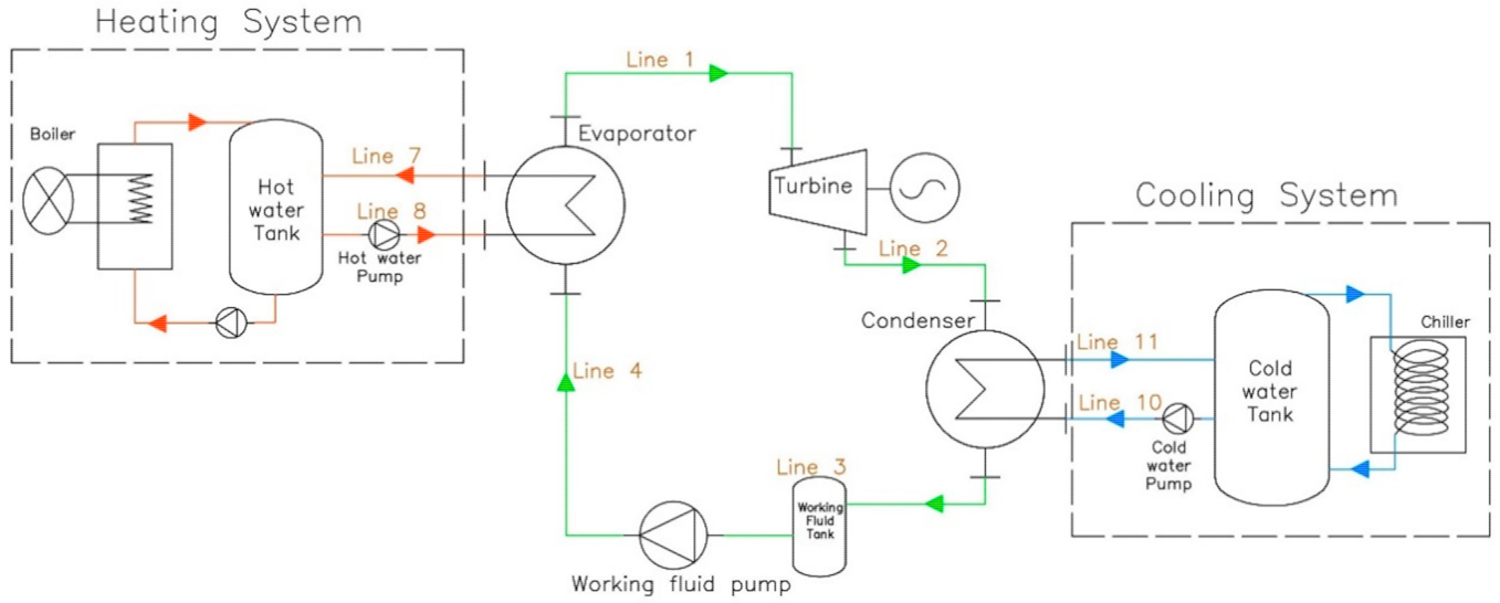
Therefore, Universidad del Caribe and Instituto de Ciencias del Mar y Limnologia, with the support of the Mexican Centre of Innovation in Ocean Energy designed and constructed the OTEC-CC-MX-1 kWe prototype, which is the first initiative in Mexico for the use and exploitation of this type of renewable energy. The prototype is located at the Universidad del Caribe in Cancun, Q. Roo. It was designed for the average surface and deep means temperatures, 27 °C and 7 °C, respectively, for the Mexican Caribbean Sea [
17]. The prototype has three systems: Rankine, Heating, and Cooling (
Figure 1). The main components of the Rankine System are the evaporator, condenser, turbine, and working fluid pump. It is worth mentioning that the working fluid is R-152a, which was selected from 50 different fluids through an evaluation that considered environmental, safety, equipment sizing characteristics, and thermal efficiency within the system [
17]. The function of the heating and cooling systems was to simulate the surface and subsurface temperatures of the Mexican Caribbean Sea. The heating system is made up of an electric heater, 1100 L tank, pressurizing pump, and 1 HP pump. The Cooling System comprises a mini chiller, centrifugal pump, and a 1100 L tank; the characteristics of the main components of the prototype are described in
Table 1.
The Rankine system operates with CC; R-152a at compressed liquid state is transported by the pump to the evaporator, where the working fluid is evaporated into a saturated vapor state by warm water from the heating system. Then, the vapor drives the turbine and the connected electrical generator to produce 1 kW of electricity. The mixture vapor from the turbine is condensed into saturated liquid state in the condenser, and then the saturated liquid of the working fluid is transported by the pump to the evaporator to begin the cycle again.
This paper presents a sensitivity analysis whose objective was to know the behavior of the OTEC-CC-MX-1 kWe prototype in design and real conditions of superficial and subsuperficial water sea temperatures to determine the non-possible operating conditions and assess the possible modifications in the prototype installation.
For this, obtaining the inlet and outlet temperatures of the water and working fluid is presented from the logarithmic mean temperatures of the plate heat exchangers using the surface and deep-water temperature data obtained for the Mexican Caribbean Sea (Exclusive Economic Zone) with Hybrid Coordinate Ocean Model (HYCOM) and Geographically Weighted Regression Temperature Model for the Mexican Caribbean Sea (GWR-TMCAS) models.
By analyzing the results, we verified maximum and minimum mass flows of water and R-152a to produce 1 kWe during a typical year in the Mexican Caribbean Sea and the conditions when the production of electricity is not possible for OTEC-CC-MX-1 kWe. Likewise, as a consequence of this analysis, a possible modification for this prototype is changing the water pump of the heating system to allow a production on 1 kWe within a wider range of temperature difference conditions.
2. Materials and Methods
2.1. Sea Temperature Estimation at Surface and 700 m Depth
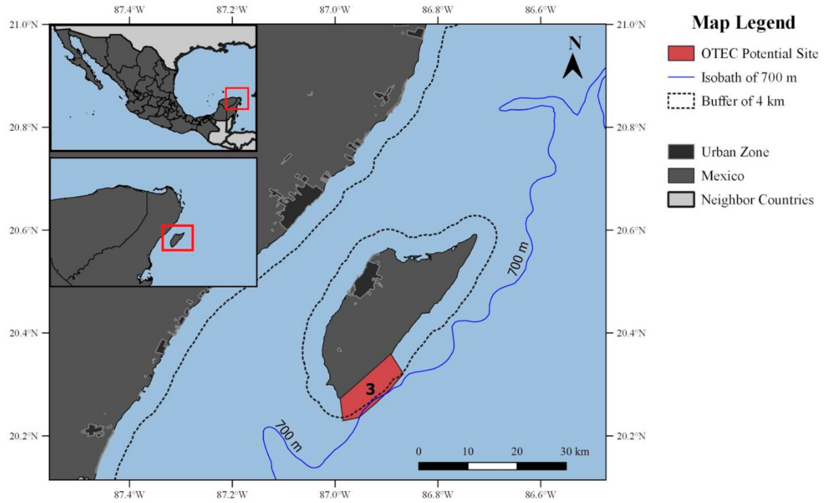
In order to estimate sea temperature difference for each month, surface and subsurface sea temperature data were obtained, considering a potential OTEC site located at the Southeast of Cozumel Island (
Figure 2). In this area, 700 m isobath is located at 4 km of the coast, and it is around 20 km away from the nearest population center. Cozumel has been assessed for OTEC prospection since 2007 [
18,
19,
20], and it was claimed that this zone has a thermal gradient higher than 20 °C along the year from a depth of 700 m.
For the sensitivity analysis, sea temperature data between 2015 and 2019 for this OTEC potential site were used. These data were grouped by month, and then mean temperatures at the surface and at 700 m depth were determined.
Monthly mean surface temperature for the OTEC potential site was obtained using the Night-time Sea Surface Temperature from National Commission to Knowledge and Use of Biodiversity (CONABIO), which have 1 km of spatial resolution and give a daily estimation of temperature [
21]. The arithmetic mean was calculated for each month using all pixel values in the raster.
Subsurface temperature data at 700 m were obtained using two different estimation models: (1) the Hybrid Coordinate Ocean Model (HYCOM) and (2) the Geographically Weighted Regression Temperature Model for the Mexican Caribbean Sea (GWR-TMCAS).
HYCOM provides daily estimations of sea subsurface temperature; this model uses climatology data and forcing fields to provide an estimation of ocean variables to adjust a circulation model [
22,
23]. HYCOM data were consulted in Google Earth Engine [
24], and
reduceRegion function was used to calculate the monthly mean temperature for the study area at 700 m depth.
On the other hand, GWR-TMCAS is a statistical model that was developed at Universidad del Caribe; it was adjusted to predict the temperature at different depths on the Mexican Caribbean Sea using variables such as latitude, longitude, month, sea surface temperature, and depth. It showed an improvement to estimated subsurface temperature in comparison with other available products for the Mexican Caribbean Sea. To run GWR-TMCAS, random points were set on the OTEC potential site to obtain initial variables for the model. With these data, arithmetic mean temperature at 700 m for each month was determined.
2.2. Inlet and Outlet Temperatures in Heat Exchangers
Once sea temperature at the surface and at 700 m depth for each month were established, logarithmic mean temperature difference (
LMTD) of the OTEC-CC-MX-1 kWe prototype heat exchangers were used to determine the inlet and outlet temperature of the working fluid and water (Equation (1)). It is worth pointing out that
LMTD according to each heat exchanger technical data was considered as constant; these values are 8.5 °C for the evaporator and 3.5 °C for the condenser.
where:
Tx: Temperature of the fluid at line
x (°C), where
x is between 1 to 11, according to
Figure 1.
Due to LMTD having multiple solutions for inlet and outlet temperatures, an algorithm for optimized inlet and outlet temperature selection was performed in Python. Considering that:
T7 is equal to the mean sea surface temperature for month i.
T10 is equal to mean sea temperature at 700 m depth for month i.
In the condenser, the working fluid just changes phase from liquid-vapor mixture to saturated liquid at the same temperature; therefore, T2 = T3.
Working fluid phase in the evaporator entrance is subcooled liquid at the same temperature as the outlet condenser working fluid temperature. Thus, T2 = T3 = T4.
The LMTDs in the evaporator and in the condenser are 8.5 °C and 3.5 °C, respectively.
The first step of the algorithm was to determine the possible combination of T2, T3, T10, and T11 in which LMTD was equal to 3.5 °C. Firstly, using T10, the range of possible values for T2, T3, and T11 was set. Secondly, all possible combinations of T2, T3, T10, and T11 were iterated; this vector was called CW. Then, LMTD for each iteration was calculated, and those where LMTD was not equal to 3.5 °C were dismissed and the CW vector was actualized.
The next step was to determine the possible combination of T1, T4, T7, and T8, in which LMTD was equal to 8.5 °C, using T7 and the range of T1 from the previous step. First, all possible combinations of T1, T4, T7, and T8 were iterated (this vector was called HW), and later, LMTD for each iteration was calculated. Combinations in which LMTD was equal to 8.5 °C were merged with the combination of inlet and outlet temperatures in the condenser that were not dismissed, in order to obtain all the inlet and outlet temperatures combination for the heat exchanger that satisfies LMTD.
This process was repeated for each surface and subsurface sea mean temperature for each month and for each surface estimation model. The diagram of the algorithm is shown in
Figure 3.
2.3. Mass and Energy Balance
Once all possible inlet and outlet temperatures for surface and subsurface sea temperature data were determined, mass and energy balance of prototype was carried out using a Python library called CoolProp [
25] and considering (1) stationary operating conditions, (2) insignificant kinetic and potential energy changes.
2.3.1. OTEC Closed Cycle
Mass and energy OTEC closed cycle was performed, taking into account pipe lines shown in
Figure 1. First, to obtained turbine real work per mass unit (
), Equation (2) was calculated.
where
is specific enthalpy of working fluid in line 1, which was determined considering working fluid as saturated vapor at
T1. To obtain real specific enthalpy in line 2 (
), turbine efficiency (
) is required as well as isoentropic specific enthalpy in line 2 (
), considering R152a as a liquid-vapor mixture at
T2.
It must be highlighted that the turbine for this prototype was designed specifically for Mexican Caribbean Sea temperature conditions, for R-152a as the working fluid and for giving 1 kW of electric power. Therefore, according to the conceptual design of this turbine, was set to 70%.
OTEC-CC-MX-1 kWe power output design (
) is 1 kWe and generator efficiency (
) is 90%, and working-fluid mass flow (
) is calculated with Equation (3).
Heat exchanged in the condenser (
) and in the evaporator (
) are calculated then using Equation (4) and Equation (5), respectively.
is specific enthalpy of working fluid in line 3, which was determined considering working fluid as a saturated liquid at T3. Meanwhile, is specific enthalpy of working fluid in line 3, which was determined considering saturated pressure of working fluid at T3 and specific entropy at line 3. This last one was determined considering working fluid as saturated liquid at T3.
Working fluid pump work (
) was calculated using Equation (6), where working fluid pump efficiency (
) is considered as 70%. This value and
were established from the previous basic engineering design of this prototype, which were set according to an extended revision of efficiency for this type of components [
26,
27]
Carnot efficiency (
) was obtained through Equation (7) and thermal efficiency (
) through Equation (8)
These calculations were made for all possible inlet and outlet temperature combinations that were obtained in the procedure described in
Section 2.2; these iterations are represented with subindex
i in each equation above.
2.3.2. Water Mass Fluxes
Taking into consideration that the same amount of heat exchanged for the working fluid in the condenser (
) and in the evaporator (
) is transferred to water and pressure drop in each exchanger, water mass fluxes for the condenser (
) and for the evaporator (
) were determined using the difference between inlet and outlet enthalpy for each heat exchanger (Equations (9) and (10)). Subindex
i represent that these calculations were made for all possible inlet and outlet temperature combination.
is specific enthalpy of water in line
x, where
x can be line 7, 8, 10, and 11 of
Figure 1.
was calculated according to water state in line
x, which was determined using water temperature (
T7,
T8,
T10, or
T11) and pressure in that line (P
7, P
8, P
10, or P
11).
Outlet pressure for both heat exchangers (P7 for the evaporator and P10 for the condenser) were considered as atmospheric pressure (101.325 kPa). Thus, inlet pressure for the evaporator (P8) was set to 173.1 kPa, and outlet pressure for the condenser was set to 131.8 kPa, due to, according to heat exchanger technical data, drop pressure at the condenser on the water side being 71.78 kPa, while drop pressure at the evaporator on the water side is 30.45 kPa.
This procedure was repeated for each inlet and outlet temperature combination obtained in the algorithm that was described in
Section 2.2 for each month and for each temperature estimation model.
2.3.3. Power Output Regarding Sea Temperature Difference
Another evaluation that was performed was the analysis of maximum power output (
) that OTEC-CC-MX-1 kWe provides regarding sea temperature difference with mass flow limits of the working fluid pump. Firstly, maximum (
) and minimum (
) volume flow of the working fluid pump (
Table 1) were used to determine the maximum (
) and minimum (
) mass flow in the OTEC cycle (Equations (11) and (12)). Subindex
i represents that these calculations were made for all possible inlet and outlet temperatures combination.
where
is working fluid density at line 3 of
Figure 1, and
was determined considering working fluid as saturated liquid at
T3.
Once was calculated for each inlet and outlet temperatures combination, Equation (3) was solved in order to find and determine and , due to these last two being used to obtain and , respectively (Equations (3) and (4)).
2.4. Best Performance Selection
When mass and energy balance results of all possible inlet and outlet temperatures were obtained, water pumps maximum flow capacity of each auxiliary system were used to filter to ones that are possible regarding OTEC-CC-MX-1 kWe operating limits.
In this sense, inlet and outlet temperature combination with a > 3.7 kg/s and > 2.8 kg/s were removed, as well as those combinations where was higher than . Then, from the rest of inlet and outlet temperatures combinations, the one with the highest was selected. This evaluation and selection were set for each month and for each estimation model.
3. Results and Discussion
As was mentioned before, the main objective of this sensitivity analysis is to know, before carrying out the experimental tests, the behavior of the OTEC-CC-MX-1 kWe prototype in design conditions of superficial (27 °C) and subsuperficial (7 °C) water sea temperature and for the surface and subsurface water temperatures of the Mexican Caribbean Sea averaged monthly over 5 years to determine the non-possible operating conditions to assess the possible modifications in the prototype installation.
This section included (1) inlet and outlet temperatures obtained from the optimization algorithm for HYCOM and GWR-TMCAS subsuperficial temperature estimations and (2) water and working fluid fluxes for these temperatures according to operational data of the pumps. Furthermore, limits of turbine operation regarding temperature difference are presented, which will be verified during OTEC-CC-MX-1 kWe experimental tests.
3.1. Inlet and Outlet Temperature for Each Model
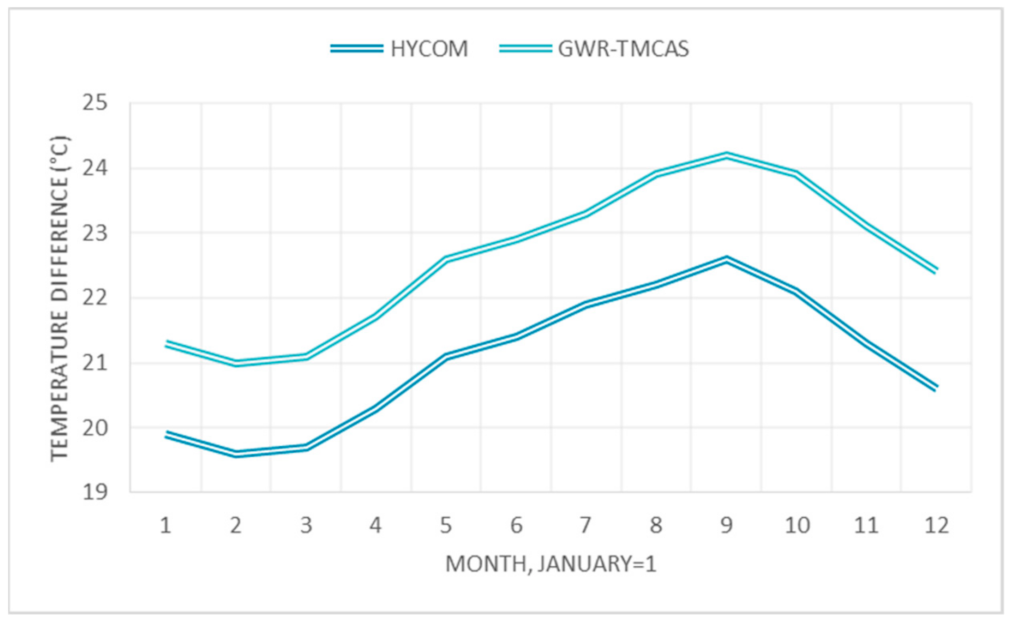
Temperature differences throughout the year for each model are presented in
Figure 4. The temperature difference was calculated using 0 (
T7) and 700 m depth (
T10) mean temperatures for each month in the study area. In general, it is evident that GWR-TMCAS estimated a larger temperature difference than HYCOM every month. Nevertheless, the minimum and temperature difference occurs in February for both models, with a value of 19.6 °C for HYCOM and 21.0 °C for GWR-TMCAS. Similar to minimum temperature difference, the maximum temperature difference is presented in the same month for both models: temperature difference in October reaches 22.6 °C for HYCOM, while GWR-TMCAS reaches 24.2 °C.
After the optimization algorithm was run for every
T7 and
T10, inlet and outlet temperatures that provide the highest
within OTEC-CC-MX-1 kWe operation limits were determined and they are shown in
Appendix A.
3.2. Mass and Energy Balance
After inlet and outlet temperatures were determined, which are described in the section above, mass and energy balance analysis were performed. The main results for each model are presented in the following graphs.
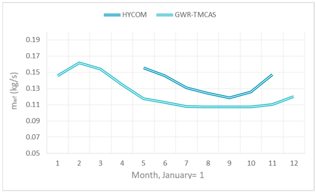
Figure 5 illustrates the
required for each month to obtain 1 kW of
. Generally,
has an inverse relationship with temperature difference. In the case of HYCOM, there are no data available for January, February, March, April, and December, due to the temperature difference estimated for this model in these months not being enough to provide 1 kW of
regarding prototype water pump limits. Therefore, until the temperature difference reached 21.0 °C (May), the mass and energy balance could be performed. Although using the actual prototype configuration is not possible to produce 1 kW of electricity with certain surface and subsurface temperatures, in the following section, it is shown that it is possible to produce less than 1 kW if it is used at the lowest mass flow rate for the working fluid. However, water pumps could be changed for further evaluations, such as using water flow as an independent variable for measuring prototype electric energy production.
In contrast, GWT-TMCAS did not have this problem due to its temperature difference being up to 21 °C every month. For this estimation model, the higher is required in February at 0.1617 kg/s, and the lower is required at 0.1072 kg/s in August, September, and October. This last value remains steady during these months due to the working fluid pump minimum volume flow limit.
A computerized calculation method was developed to obtain the generated net power of an OTEC plant taking into account water pipe diameter, warm and cold seawater temperature, and mass flow rate of seawater. In that study, they noted that when they fixed warm seawater temperature and pipe diameter, a larger rate of working fluid was required for a lower temperature difference [
28].
In addition, a sensitivity analysis was done of a 100 MW CC-OTEC plant to estimate net power and efficiency regarding variations of water velocity, water temperature, and water pipe diameter, and a direct relationship was found between water mass flow and working fluid mass flow, which means that decreasing water mass flow will lower the working fluid mass flow as well [
29]. This relation can be seen by comparing
Figure 5 and
Figure 6 in certain months such as August in GWR-TMCAS. Nevertheless, it is not evident for all months: this behavior can be caused by the OTEC-CC-MX-1 kWe water pump limits and by optimization of inlet and outlet temperatures.
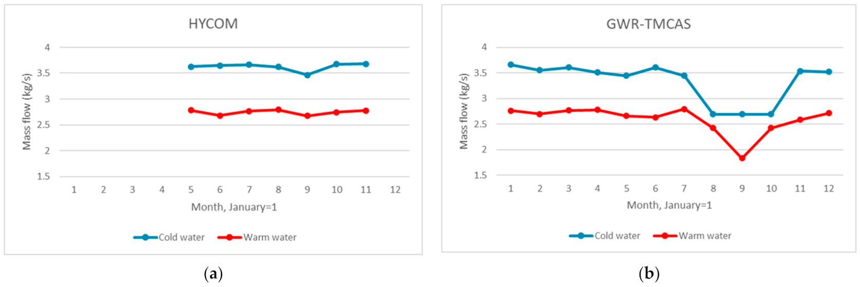
Figure 6 shows
and
for each model throughout the year. As well as
, only data between May and November are available for HYCOM. In these months, both mass fluxes seem to stay stable, and
fluctuates between 3.68 and 3.47 kg/s, while
fluctuates between 2.67 and 2.79 kg/s.
For GWR-TMCAS, and fluctuations are more remarkable. for this model has a sharp drop between August and October, when remains steady, and value reaches around 2.69 kg/s. In the same way, also has a fall, but it is more considerable than the decline in . decreases to 1.84 kg/s in September, when the maximum temperature difference is presented.
Owing to OTEC-CC-MX-1 kWe preliminary design, the amount of
is greater than
, as is seen in
Figure 6. In this prototype,
/
was not taken into account for design due to OTEC-CC-MX-1 kWe being built for laboratory scale. However, when a CC-OTEC plant is designed with a capacity greater than 50 MW, it is recommended that
/
be above 1, because of the distance to the cold water sink from the OTEC platform. If
/
> 1, more power would be required to pump cold water at 1000 m depth, and therefore, power net output would be lower [
30].
Supporting this idea, the authors of [
28] found that power net output seems to increase with
/
, and the authors of [
31] also found that net power output increases sharply by increasing
; nevertheless, the increment velocity slows down which might be caused by heat exchangers performance. For further investigation, new water pump calculations could be carried out in order to consider the optimized algorithm described above to determine inlet and outlet temperatures and to fluctuate water mass flow as another parameter for OTEC-CC-MX-1 kWe sensitivity analysis.
Another variable that was evaluated is
; its variation along the year for both models arise shown in
Figure 7, where it can be seen how
has a direct relationship with temperature difference. Maximum
for HYCOM is presented in September with a value of 3.04%; otherwise the minimum
is presented in May with a value of 2.34%. Similarly, maximum
for GWR-TMCAS occurs in the months with the higher temperature difference (August, September, and October), and it remains steady at 3.35% due to OTEC-CC-MX-1 kWe components limitations. Minimum
for GWR-TMCAS is 2.25%, which occurs in February.
3.3. Efficiency Regarding Temperature Difference
The last evaluation made for this sensitivity analysis is the maximum
that OTEC-CC-MX-1 kWe provides regarding sea temperature difference, considering minimum and maximum working fluid mass flow according to the technical specification of this pump. For the minimum and maximum flow,
equal to 1.34 × 10
−4 m
3/s and
equal to 1.34 × 10
−3 m
3/s were considered, respectively. Inlet and outlet temperatures for each model obtained with the optimized algorithm are presented in
Appendix B.
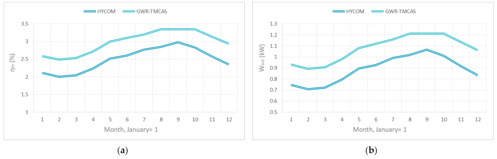
Variation of
and
in each month for each model, considering that
is shown in
Figure 8. Overall,
and
increase when temperature difference increases, so minimum
and minimum
are presented in February, and maximum
and maximum
are presented in September.
For HYCOM, fluctuates between 2% and 2.89%, and fluctuates between 0.71 kW and 1.06 kW. For GWR-TMCAS, fluctuates between 2.49% and 3.45%, and fluctuates between 0.89 kW and 1.21 kW.
For this last model, and maintain the same level during August, September, and October, despite the difference temperature increase; consequently, the values for these variables in these months seem to be the maximum values possible for OTEC-CC-MX-1 kWe prototype due to the components’ operation limits.
This behavior is similar to behavior shown in
Figure 7, because during months with the highest and lowest thermal differences, the highest and lowest values for thermal efficiency are obtained, respectively.
A relationship between water temperature and power output was found by [
28], who explained that a larger temperature difference between heat source and sink leads to higher efficiency of the OTEC plant, depending on its components’ limits as well.
In addition, the authors of [
29] found that an increase in warm water temperature leads to an improvement of net power and efficiency. In contrast, an increment in cold water temperature leads to a decrease in net power and efficiency [
29]. Similar results were found in [
32], where the performance was compared of net power output regarding different exchanger and different temperature difference.
Evaluation of and in each month for each model, considering , was not possible, due to the water pumps’ flow limits.
4. Conclusions
The aim of the present sensitivity analysis was to evaluate OTEC-CC-MX-1 kWe operation under design conditions and off-design conditions. Off-design conditions are the monthly mean sea temperature difference, which were evaluated between surface and 700 m depth sea temperature around Cozumel Island using HYCOM and GWR-TMCAS temperature estimations.
Mass and energy balance to produce 1 kWe for each off-design condition was carried out using heat exchanger LMTD to determine inlet and outlet temperatures using an optimized algorithm. Then, it water mass flow, working fluid flow, and thermal efficiency were determined for each condition, taking into account components operation limits. In addition, maximum power productions according to the lowest rate limit of working fluid pump, temperature difference range, and water pumps’ operation limits were obtained.
These analyses allowed us to know a priori prototype performance, as well as conditions when the production of electricity is not possible for OTEC-CC-MX-1 kWe. As future work, these results will be used for optimizing the prototype and carrying out the first experimental tests. To illustrate, as a consequence of this analysis, a possible modification for this prototype is changing the water pump of the heating system in order to use HYCOM temperature data for the months where it was not possible to produce 1 kWe. In addition, hot water flow could be used as an independent variable for measuring prototype energy production in further evaluations.


