The Cost of Photovoltaic Forecasting Errors in Microgrid Control with Peak Pricing

Abstract

Model predictive control (MPC) is widely used for microgrids or unit commitment due to its ability to respect the forecasts of loads and generation of renewable energies. However, while there are lots of approaches to accounting for uncertainties in these forecasts, their impact is rarely analyzed systematically. Here, we use a simplified linear state space model of a commercial building including a photovoltaic (PV) plant and real-world data from a 30 day period in 2020. PV predictions are derived from weather forecasts and industry peak pricing is assumed. The effect of prediction accuracy on the resulting cost is evaluated by multiple simulations with different prediction errors and initial conditions. Analysis shows a mainly linear correlation, while the exact shape depends on the treatment of predictions at the current time step. Furthermore, despite a time horizon of 24 h, only the prediction accuracy of the first 75 min was relevant for the presented setting.

1. Introduction

The control of microgrids has gained huge attention in the research community within the last decade. One of the most popular methods is model predictive control (MPC). Its task is to find optimal control sequences for power generation and distribution, thereby including forecasts of external conditions such as load demands, renewable energy sources and electricity pricing. However, these forecasts are always subject to uncertainties. Different strategies to handle these uncertainties exist, e.g., robust [1,2] or stochastic [3,4,5] MPC. Essentially, their aim is to either ensure stability and/or constraint satisfaction (in case of robust MPC), or to minimize a stochastic entity, such as the expected value of costs (in case of stochastic MPC). The literature on different MPC approaches for microgrid control is rich and includes various models, optimization goals and such strategies, see, e.g., the reviews [6,7,8].

However, the urgency of handling uncertainties depends on their impact, which, again, might depend heavily on the respective application. Specifically, the most common objective, monetary cost, varies with different pricing structures. With the high peak costs encountered in German industry pricing, for example, forecasting errors can have serious consequences. Thus, a systematic analysis of how (realistic) forecasting errors affect the control outcome is necessary.

One important source of uncertainties in modern microgrids is the use of photovoltaic (PV) plants as renewable energy sources. While their power production can be predicted from widely available weather forecasts [9,10], simulation studies with real-world predictions are comparatively rare. Mostly, strategies to handle uncertainties are presented, and the effect of forecasting errors themselves is only investigated in the evaluation of the new strategy.

An interesting example of an application using historical weather forecasts as predictions for the PV production is [11]. The uncertainties are accounted for by a stochastic MPC approach with chance constraints. The stochastic MPC outperforms a deterministic MPC, but the relationship between the forecasting error and the resulting additional energy use remains unclear. The effect of PV and wind power production forecasts on their integration in the German power grid is considered in [12]. Namely, the resulting control reserve power, the regime switches per week (i.e., how often a storage has to change between charging and discharging) and the storage energy losses are evaluated. However, the authors come to the conclusion that today’s forecasts are sufficient and further improvement would have no significant effects. In [13], an affine arithmetic method for microgrid control is introduced and compared, among others, to MPC methods. Three different levels of artificial forecasting errors are considered, for which the error increases linearly within the time horizon (but with three different slopes). The numerical results show that, for regular MPC, costs increase significantly with the error (level). In [14], a residential home with plannable loads and PV and wind energy sources is controlled. Five different levels of uniformly distributed forecasting errors from 6% to 30% are respected, resulting in increasing costs. In [15], a microgrid with intraday pricing is considered. Simulation results suggest a perfectly linear relation between a forecast error, varied between 19% and 21% and costs. However, this cost increase seems negligible in comparison to additional costs from forecasting errors on electricity prices. In [16], a microgrid is controlled in a rolling horizon fashion with forecasts for both PV production and load demand. The authors scale the prediction error and show that the resulting operation costs increase more strongly than the linear with the normalized root mean square error of the forecasts. Costs arise from fuel consumption and the number of generator start-ups. In [17], a microgrid with forecasts for electricity prices, load demand, PV and wind power generation is controlled using MPC. The forecasting error for PV generation is varied from 8 to 24%. However, the results suggest no significant effect. In [18], an AC/DC microgrid model with a wind turbine and a PV plant is controlled in real-time. Reference points for power generation and use under uncertain forecasts are derived by a robust optimization of a mixed-integer linear programming problem [19]. Forecast uncertainties are respected by possible variations in $\pm 2\%$ of power generation. Simulation results show an increase in total costs over the $200\mathrm{s}$ simulation period of $12.45\%$ for the worst-case scenario. In [20], a microgrid with multiple distributed generators and storages is controlled. Using dual decomposition, the optimization problem can be solved by a distributed algorithm. Uncertainties in wind forecasts are robustly respected by minimizing the worst-case transaction cost. However, no analysis of the cost impact on the dependence of the uncertainty is conducted. In [21], a closed-loop robust MPC approach is developed for the control of a building with uncertain heat gains. The effect of different uncertainty levels on thermal discomfort and energy usage is evaluated for the proposed approach and the use of open-loop robust MPC and only regular MPC. The robust MPC approaches are effective in reducing thermal comforts; however, this leads to an expense of energy usage. In [22], this closed-loop robust MPC is approach is used for temperature control of a single room. In a comparison with regular MPC and a rule-based controller, it shows superior results only for an intermediate level of uncertainty (30–67%). With less uncertainty, the regular MPC is advantageous and for higher uncertainty, the rule-based controller is advantageous. In [23], different MPC variants are compared for the temperature control of a building. While the simulated thermal sensation of the inhabitants deteriorates with an increasing level of uncertainty for all control schemes, the energy usage shows no clear trend and varies by less than $1\%$. In [24], a stochastic MPC approach is used to control the heating, ventilation and air conditioning (HVAC) unit and zone temperature of a building. For the uncertain loads (outside air temperature and occupancy), probability distributions are derived from historical data. Then, the expected energy usage is minimized while satisfying chance constraints. The stochastic MPC approach is compared to a standard MPC, which uses expected load values. The results suggest superiority of the stochastic MPC, if the uncertainty level is not too high, i.e., if the forecasting errors are scaled with a factor ≤ 5. In [25], stochastic MPC with explicit chance constraints is used for demand response in a residential energy management system. Uncertainties in PV power production and ambient temperature are modeled as normally distributed. A doubling of the standard deviation of the PV forecasting error leads to an increase in necessary grid power reduction of $\approx 43\%$.

While most work shows a significant increase in cost for increasing errors, its form remains unclear [11,13,14,18,21,22,24,25]. Or, if the relationship is investigated, peak costs are not included in the electricity pricing scheme [15,16]. Real forecasting data are used in [11,16,20], while most works only use artificial errors [12,13,14,15,17,18,21,22,23,25]. Furthermore, there is no investigation into the necessary time horizon length for predictions, i.e., on which time scale the prediction accuracy is relevant.

In summary, while there are many approaches to address uncertainties in predictive microgrid control, we see a gap in research into the effect of realistic uncertainties if unhandled, especially for the challenging case of peak costs. However, this is crucial for the assessment of investments in forecasting technologies. Thus, we try to answer the following questions:

• Are state-of-the-art weather predictions already sufficient to reduce demand peaks?
• What is the correlation between prediction accuracy and resulting cost?
• What is the time horizon in which the prediction accuracy is relevant?

To address them, we first describe a linear state space model of a microgrid, an economic MPC approach for its control, and real-world data used for simulation, as well as how we adjust the prediction errors from weather forecasts, in Section 2. We investigate the operational cost of the microgrid for a 30-day period from 2020 for various settings in Section 3. These include different initial peaks (i.e., limits from which peak costs occur), prediction errors, assumed knowledge of PV production at the current time step and different forecasting errors at the beginning of the prediction horizon.

As our main contributions, we show that, for a realistic microgrid setting of a medium-sized company building with real-world data:

• Using solar irradiance forecasts from weather services as predictions for PV power generation can reduce peak costs;
• The cost reduction scales with the prediction error, specifically

  –

  If PV generation is known at the current time step, the costs increase linearly with the prediction error;

  –

  If only predictions are used for the current time step, the correlation resembles a piece-wise linear function, with a significantly higher slope for lower errors.

• Our results suggest that the prediction accuracy for PV generation is only relevant within a short period at the beginning of the prediction horizon.

2. Methodology and Simulation Setup

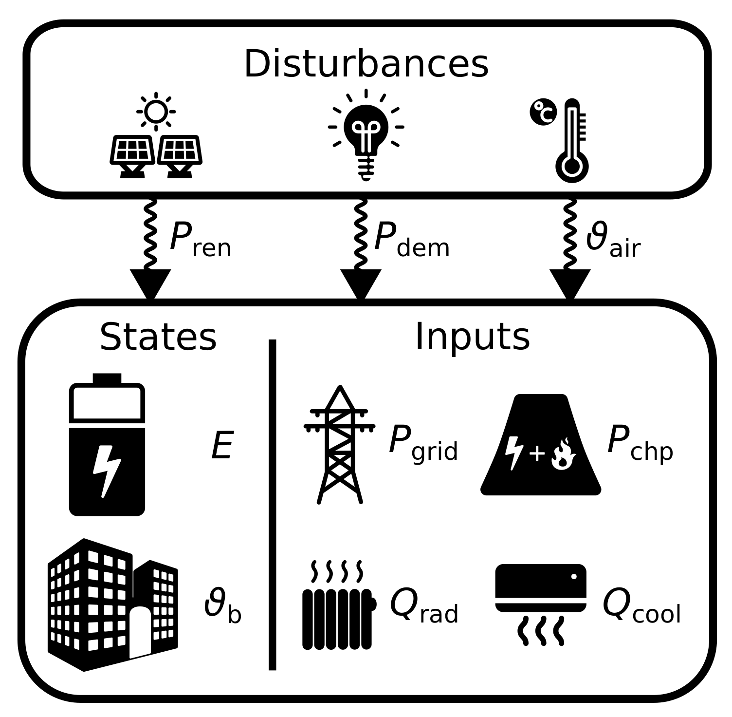
2.1. Microgrid Modeling

The microgrid represents a medium-sized office building in Offenbach, Germany, and is given as a discrete-time linear state space model of the form

$$\begin{array}{c}x(k+1)=Ax\left(k\right)+Bu\left(k\right)+Sd\left(k\right).\end{array}$$

(1)

The state vector x consists of the stored energy of a battery E and the building temperature ${\vartheta }_{\mathrm{b}}$. The inputs u are the power bought from/sold to the grid $P_{\mathrm{grid}}$, the power produced by a combined heat and power plant (CHP) $P_{\mathrm{chp}}$ and heating (${\dot{Q}}_{\mathrm{rad}}$) and cooling (${\dot{Q}}_{\mathrm{cool}}$) power from a heating, ventilation and air conditioning system. Influences which cannot be controlled are modeled as disturbances d, i.e., the generated PV power $P_{\mathrm{ren}}$, the load demand $P_{\mathrm{dem}}$ and the ambient air temperature ${\vartheta }_{\mathrm{air}}$. Figure 1 shows an overview of the microgrid’s structure.

The state dynamics are given by

$$\begin{gathered} \left[\begin{array}{c}{E}_{(}k+1)\\ {\vartheta }_{\mathrm{b}}(k+1)\end{array}\right]=\left[\begin{array}{cc}1& 0\\ 0& -e^{\frac{-H_{\mathrm{air}}}{C_{\mathrm{th}}}{T}_{\mathrm{s}}}\end{array}\right]·\left[\begin{array}{c}{E}_{(}k)\\ {\vartheta }_{\mathrm{b}}\left(k\right)\end{array}\right]+\left[\begin{array}{cccc}{T}_{\mathrm{s}}& T_{\mathrm{s}}& 0& \frac{T_{\mathrm{s}}}{{\epsilon }_{\mathrm{c}}}\\ 0& \frac{\mu }{c_{\mathrm{cur}}}& \mu & \mu \end{array}\right]·\left[\begin{array}{c}{P}_{\mathrm{grid}}\left(k\right)\\ P_{\mathrm{chp}}\left(k\right)\\ {\dot{Q}}_{\mathrm{rad}}\left(k\right)\\ {\dot{Q}}_{\mathrm{cool}}\left(k\right)\end{array}\right]\dots \\ +\left[\begin{array}{ccc}{T}_{\mathrm{s}}& T_{\mathrm{s}}& 0\\ 0& 0& H_{\mathrm{air}}·\mu \end{array}\right]·\left[\begin{array}{c}{P}_{\mathrm{ren}}\left(k\right)\\ P_{\mathrm{dem}}\left(k\right)\\ {\vartheta }_{\mathrm{air}}\left(k\right)\end{array}\right], \end{gathered}$$

(2)

where $\mu =\frac{1-e^{-\frac{H_{\mathrm{air}}}{C_{\mathrm{th}}}{T}_{\mathrm{s}}}}{H_{\mathrm{air}}}$. Electrical powers are denoted by P and thermal powers by Q. For details of the modeling, the reader is referred to [26]. Note that the battery charging power $P_{\mathrm{charge}}$ is no input on its own, but is implicitly given by $P_{\mathrm{charge}}\left(k\right)=E_{(}k+1)-E_{(}k)$, see (7). The model parameters are given in

Table 1. Building model parameters for System (2).

Parameter	Description	Value
$T_{\mathrm{s}}$	Sample time (step width) in h	0.25, 0.5 or 1
$C_{\mathrm{th}}$	Thermal capacity of the building in kWh/K	1792.06
$H_{\mathrm{air}}$	Heat transfer coefficient to outside air in kW/K	341.94
${\epsilon }_{\mathrm{c}}$	Energy efficiency ratio cooling machine	$2.5$
$c_{\mathrm{cur}}$	Current constant CHP, i.e., $P_{\mathrm{chp}}=c_{\mathrm{cur}}·{\dot{Q}}_{\mathrm{chp}}$	0.677

, the constraints in

Table 2. Constraints on states and inputs for System (2). In the following, we will refer to upper and lower limits by appending $\max$ and $\min$ as superscripts, respectively.

Variable	Limits	Unit
E	$[14.7,83.3]$	$\mathrm{kWh}$
${\vartheta }_{\mathrm{b}}$	$[19,23]$	°C
$P_{\mathrm{grid}}$	$[-1000,1000]$	$\mathrm{kW}$
$P_{\mathrm{chp}}$	$[0,199]$	$\mathrm{kW}$
${\dot{Q}}_{\mathrm{heat}}$	$[0,600]$	$\mathrm{kW}$
${\dot{Q}}_{\mathrm{cool}}$	$[-440,0]$	$\mathrm{kW}$
$P_{\mathrm{charge}}$	$[-32.9,32.9]$	$\mathrm{kW}$

.

2.2. Economic MPC Approach

In contrast to regular tracking MPC, in econonomic MPC, the objective function may be of an arbitrary form. In this study, we minimize three objectives. First, the desired temperature set point is ${\vartheta }_{\mathrm{set}}=$21 °C. Thus, to punish both too-high and too-low temperature values, we use the quadratic deviation as costs,

$$\begin{array}{ccc}\hfill {\ell }_{\mathrm{comf}}\left(k\right)& =\hfill & {\left({\vartheta }_{\mathrm{b}}\left(k\right)-{\vartheta }_{\mathrm{set}}\right)}^2·T_{\mathrm{s}}\left(k\right).\end{array}$$

(3)

The scaling with $T_{\mathrm{s}}\left(k\right)$ is necessary due to the varying step widths. Second, we minimize all occurring monetary costs, which stem from buying/selling power to the grid and gas costs for both CHP and gas heating. For German industry pricing, these can be described as

$$\begin{array}{}\text{(4)}& \hfill {\ell }_{\mathrm{mon}}\left(k\right)& =\hfill & \left(c_{\mathrm{chp}}·P_{\mathrm{chp}}\left(k\right)+c_{\mathrm{gas}}·{\dot{Q}}_{\mathrm{rad}}\left(k\right)\right)·T_{\mathrm{s}}\left(k\right)\hfill \text{(5)}& & \dots +\hfill & \left(c_{\mathrm{grid},\mathrm{buy}}·max\left(0,P_{\mathrm{grid}}\left(k\right)\right)-c_{\mathrm{grid},\mathrm{sell}}·max\left(0,-P_{\mathrm{grid}}\left(k\right)\right)\right)·T_{\mathrm{s}}\left(k\right)\hfill \text{(6)}& & \dots +\hfill & c_{\mathrm{grid},\mathrm{peak}}·max\left(0,P_{\mathrm{grid}}\left(k\right)-P_{\mathrm{grid},\mathrm{peak}}\left(k\right)\right),\hfill \end{array}$$

where $c_{\mathrm{chp}}$, $c_{\mathrm{gas}}$, $c_{\mathrm{grid},\mathrm{buy}}$, $c_{\mathrm{grid},\mathrm{sell}}$ and $c_{\mathrm{grid},\mathrm{peak}}$ are constants [26]. $P_{\mathrm{grid},\mathrm{peak}}\left(k\right)$ refers to the maximum peak in $P_{\mathrm{grid}}$, which has occurred until time step k. In Germany, the peak costs $c_{\mathrm{grid},\mathrm{peak}}·P_{\mathrm{grid},\mathrm{peak}}$ are evaluated annually. In other countries, they might be evaluated and reset monthly. Furthermore, they tend to increase, while $c_{\mathrm{grid},\mathrm{peak}}=100.01\frac{€}{\mathrm{kW}}$ for 2020 has already been comparatively high. Note that the max-terms in (5) and (6) can be translated into a linear expression by an epigraph reformulation (see [26] for details).

Third, we slightly punish the use of the stationary battery to prevent arbitrary charging and discharging. Otherwise, if there is no incentive to either shave peaks in $P_{\mathrm{grid}}$ or store excessive energy from $P_{\mathrm{ren}}$, there would be an infinite number of equally optimal solutions for $P_{\mathrm{grid}}$ (since no battery losses are assumed). We use a linear cost term

$$\begin{array}{ccc}\hfill {\ell }_{\mathrm{bat}}\left(k\right)& =\hfill & \left|\underset{P_{\mathrm{charge}}\left(k\right)}{\underbrace{P_{\mathrm{grid}}\left(k\right)+P_{\mathrm{chp}}\left(k\right)+\frac{{\dot{Q}}_{\mathrm{cool}}\left(k\right)}{{\epsilon }_{\mathrm{c}}}+P_{\mathrm{ren}}\left(k\right)+P_{\mathrm{dem}}\left(k\right)}}\right|·T_{\mathrm{s}}\left(k\right),\end{array}$$

(7)

where the absolute value $|·|$ can again be translated into a linear expression by an epigraph reformulation. The prediction horizon has an overall length of $24\mathrm{h}$, split into 56 steps. However, since forecast accuracy decreases with time, we sample the first $8\mathrm{h}$ window denser than the middle and last interval,

$$\begin{array}{ccc}\hfill T_{\mathrm{s}}\left(k\right)& =\hfill & \left\{\begin{array}{cc}0.25\mathrm{h}\hfill & \mathrm{if}k\in [0,31],\hfill \\ 0.5\mathrm{h}\hfill & \mathrm{if}k\in [32,47],\hfill \\ 1\mathrm{h}\hfill & \mathrm{if}k\in [48,55].\hfill \end{array}\right.\end{array}$$

(8)

The overall objective function, which is minimized at every time step, i.e., every $15\min$, is then given by

$$\begin{array}{ccc}\hfill J_{\mathrm{opt}}& =\hfill & {\displaystyle \sum _{k=0}^{N_{\mathrm{p}}-1}}{w}_{\mathrm{comf}}·{\ell }_{\mathrm{comf}}(x\left(k\right),u\left(k\right))+w_{\mathrm{mon}}·{\ell }_{\mathrm{mon}}\left(u\left(k\right)\right)+w_{\mathrm{bat}}·{\ell }_{\mathrm{bat}}\left(u\left(k\right)\right).\end{array}$$

(9)

The weights $w_{\mathrm{comf}}$ and $w_{\mathrm{mon}}$ have been derived from 2D Pareto optimization over a longer time periods [26,27]. $w_{\mathrm{bat}}$ is then chosen to be large enough to prevent the arbitrary charging and discharging of the battery, but small enough to keep the rewarding incentives of battery use described above.

2.3. Simulation Framework

2.3.1. Data Sources

We use the real-world data of a medium-sized office building in Germany, recorded over 30 days, starting from 14 April 2020. The building contains a comparatively large PV plant, such that the effective power demand $P_{\mathrm{ren}}+P_{\mathrm{dem}}$ has negative peaks on most days, see Figure 2.

For this study, perfect knowledge of building demand $P_{\mathrm{dem}}$ and outside air temperature ${\vartheta }_{\mathrm{air}}$ is assumed. For PV power production $P_{\mathrm{ren}}$, real-world forecasts of the solar irradiance $I_{\mathrm{sol}}$ from a commercial weather service are used. Forecasts are updated every ≈65 min. The real values were measured with an on-site weather station.

The solar irradiance $I_{\mathrm{sol}}$ has to be converted into the PV power output $P_{\mathrm{ren}}$. In general, the relationship can be described by

$$\begin{array}{ccc}\hfill {\tilde{P}}_{\mathrm{ren}}& =\hfill & {\eta }_{\mathrm{PV}}·A_{\mathrm{PV}}·I_{\mathrm{sol}}·\left(1-\beta (T_{\mathrm{cell}}-25°\mathrm{C})\right),\end{array}$$

(10)

with ${\eta }_{\mathrm{PV}}$ being the reference efficiency, $A_{\mathrm{PV}}$ the surface area, $T_{\mathrm{cell}}$ the operating temperature of the cell and a constant $\beta \approx 0.04$ [28]. For the purpose of this study, we neglect the temperature influence, resulting in the linear approximation

$$\begin{array}{ccc}\hfill P_{\mathrm{ren}}\left(k\right)& =\hfill & {\eta }_{\mathrm{PV}}·A_{\mathrm{PV}}·I_{\mathrm{sol}}\left(k\right).\end{array}$$

(11)

Figure 3 shows the true trajectory of $I_{\mathrm{sol}}$ for two days together with different forecasts.

2.3.2. Artificial Errors

To systematically analyze the effect of different prediction errors, we introduce artificial errors by scaling the actual prediction errors linearly. Let $P_{\mathrm{ren}}\left(k\right)$ be the real value at time step k and $P_{\mathrm{ren}}\left(n\right|k)$ the value of $P_{\mathrm{ren}}(n+k)$ predicted at time step k (with $n\in [0,N_{\mathrm{pred}}-1]$). Then, the new prediction with an error scale of $s_{\mathrm{err}}$ is

$$\begin{array}{ccc}\hfill P_{\mathrm{ren}}^{s_{\mathrm{err}}}\left(n\right|k)& =\hfill & min\left(max\left(P_{\mathrm{ren}}(n+k)+s_{\mathrm{err}}·\underset{\mathrm{regular}\mathrm{prediction}\mathrm{error}{e}_{\mathrm{ren}}\left(k\right)}{\underbrace{(P_{\mathrm{ren}}(n+k)-P_{\mathrm{ren}}\left(n\right|k))}},P_{\mathrm{ren}}^{\max }\right),0\right).\end{array}$$

(12)

Note that we limit predictions to stay within physical limitations, i.e, $0\le P_{\mathrm{ren}}^{s_{\mathrm{err}}}\le P_{\mathrm{ren}}^{\max }$. Thus, we use the resulting mean absolute error within the prediction horizon for the subsequent analyses. It is calculated by

$$\begin{array}{c}\hfill e_{\mathrm{avg}}\left(s_{\mathrm{err}}\right)=\frac{1}{N_{\mathrm{sim}}·N_{\mathrm{pred}}}{\displaystyle \sum _{k=1}^{N_{\mathrm{sim}}}\sum _{n=0}^{N_{\mathrm{pred}}-1}}|P_{\mathrm{ren}}^{s_{\mathrm{err}}}\left(n\right|k)-P_{\mathrm{ren}}(n+k)|,\end{array}$$

(13)

where $N_{\mathrm{sim}}$ is the total number of simulation steps.

2.3.3. Treatment of Disturbances at Current Time Step

A non-trivial challenge is the handling of predictions at the current time step. If no robust MPC approach is used, differences in predicted values $d\left(0\right|k)$ for disturbances and real values $d\left(k\right)$ lead to $x(k+1)\ne x\left(1\right|k)$, potentially violating state constraints. Figure 4 illustrates how predictions for the solar irradiance $I_{\mathrm{sol}}\left(0\right|k)$ at the current time step and its true values $I_{\mathrm{sol}}\left(k\right)$ can be different. Thus, the error $e_{\mathrm{ren}}\left(k\right)=P_{\mathrm{ren}}\left(k\right)-P_{\mathrm{ren}}\left(0\right|k)$ has to be handled, for which we propose two options.

First, in the optimistic scenario, we assume perfect measurements, i.e., $P_{\mathrm{ren}}\left(0\right|k)=P_{\mathrm{ren}}\left(k\right)$. This neglects that a measurement at time k is most likely to change within the time step (i.e., during the following $15\min$), and thus does not represent the necessary average. In this case, no further handling of $e_{\mathrm{ren}}$ is necessary and all constraints will be fulfilled.

Second, in the pessimistic scenario, we assume no additional measurement at time k, which means that we use a value which was predicted up to $65\min$ ago. We use heuristic rules to account for $e_{\mathrm{ren}}\left(k\right)$. If $e_{\mathrm{ren}}\left(k\right)>0$ (i.e., higher PV production than expected), the surplus is balanced by decreasing $P_{\mathrm{grid}}\left(k\right)$. If $e_{\mathrm{ren}}\left(k\right)<0$ (i.e., lower PV production than expected), we discharge the stationary battery if this is necessary to prevent a new peak in $P_{\mathrm{grid}}$ (while respecting all constraints). Otherwise, $P_{\mathrm{grid}}\left(k\right)$ is used to compensate $e_{\mathrm{ren}}\left(k\right)$.

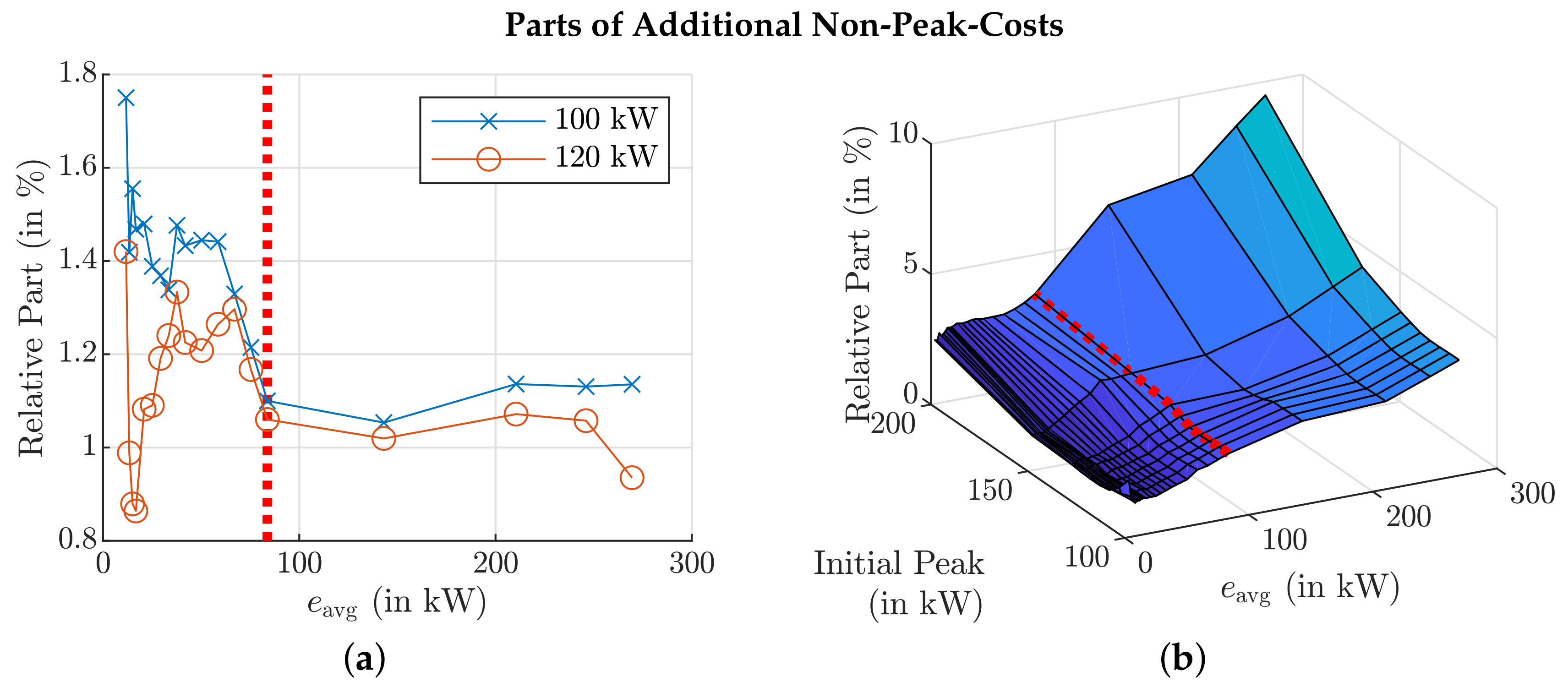
3. Results & Discussion

Both model and control algorithms from Section 2 were implemented in PARODIS [29] (available at https://github.com/teamparodis/parodis, accessed on 24 April 2020), which is an easy-to-use general MPC framework for Matlab and builds upon YALMIP [30]. With GUROBI as the solver, a single simulation of 30 days takes ≈ 150 s on an Intel i7-8550U notebook CPU.

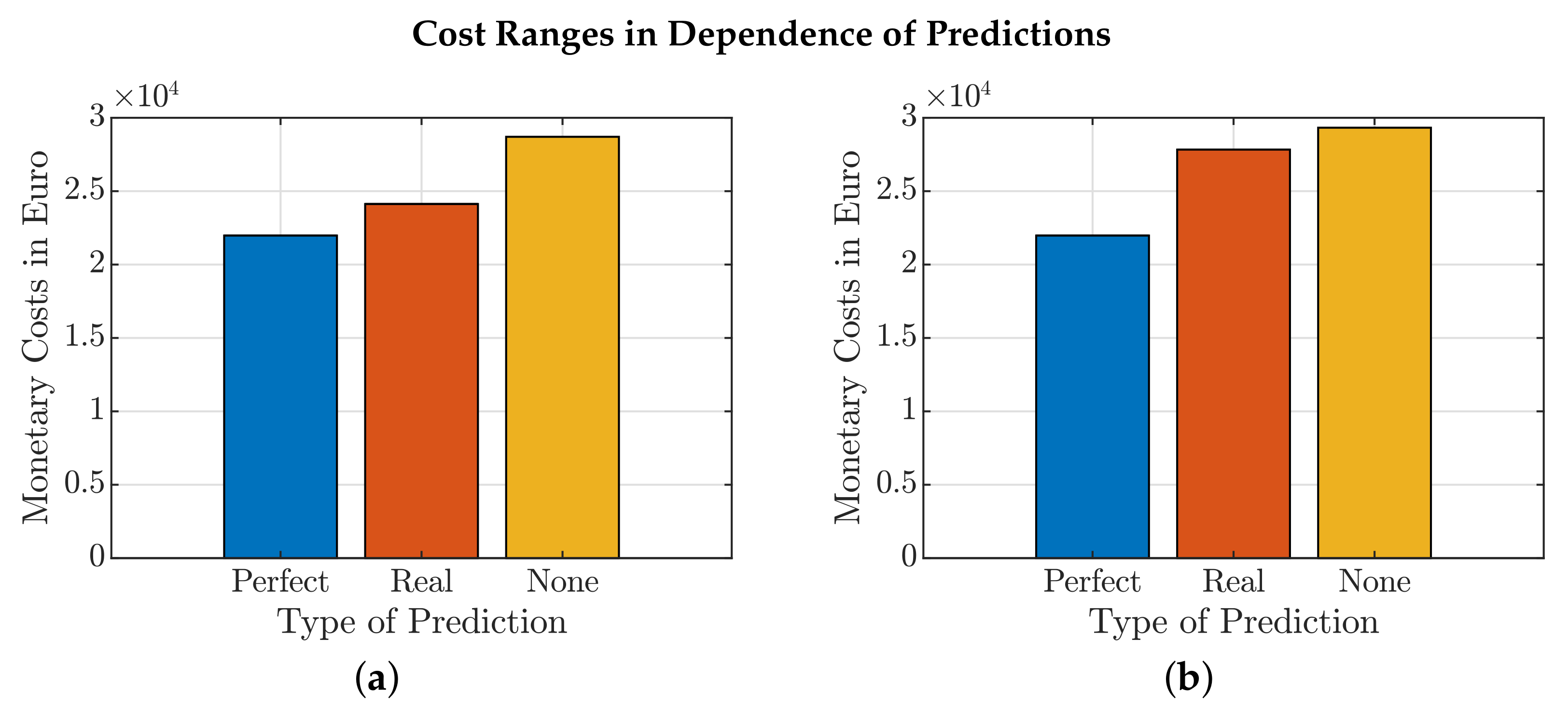
3.1. Potential Savings

The general potential savings, i.e., the difference in cost between simulation with no and with perfect predictions, are shown for both scenarios (optimistic and pessimistic) in Figure 5.

Assuming perfect predictions, the minimum monetary costs for the 30-day period are 21,980€ (including, however, the entire peak cost for the initially assumed peak of $100\mathrm{kW}$). If no predictions for $P_{\mathrm{ren}}$ are used (i.e., $P_{\mathrm{ren}}\left(n\right|k)=0\forall n\in [0,N_{\mathrm{pred}}-1]$), they increase to 28,704€ or 29,324€ for the optimistic and pessimistic scenario, respectively. For the optimistic scenario, this results in potential savings of 6724€, and we already reach 4577€ with our current prediction quality. However, for the pessimistic scenario, we only reach savings of 1491€ out of the potential 7344€. This leads to the following question: how good would the predictions need to be to achieve a certain amount of potential savings?

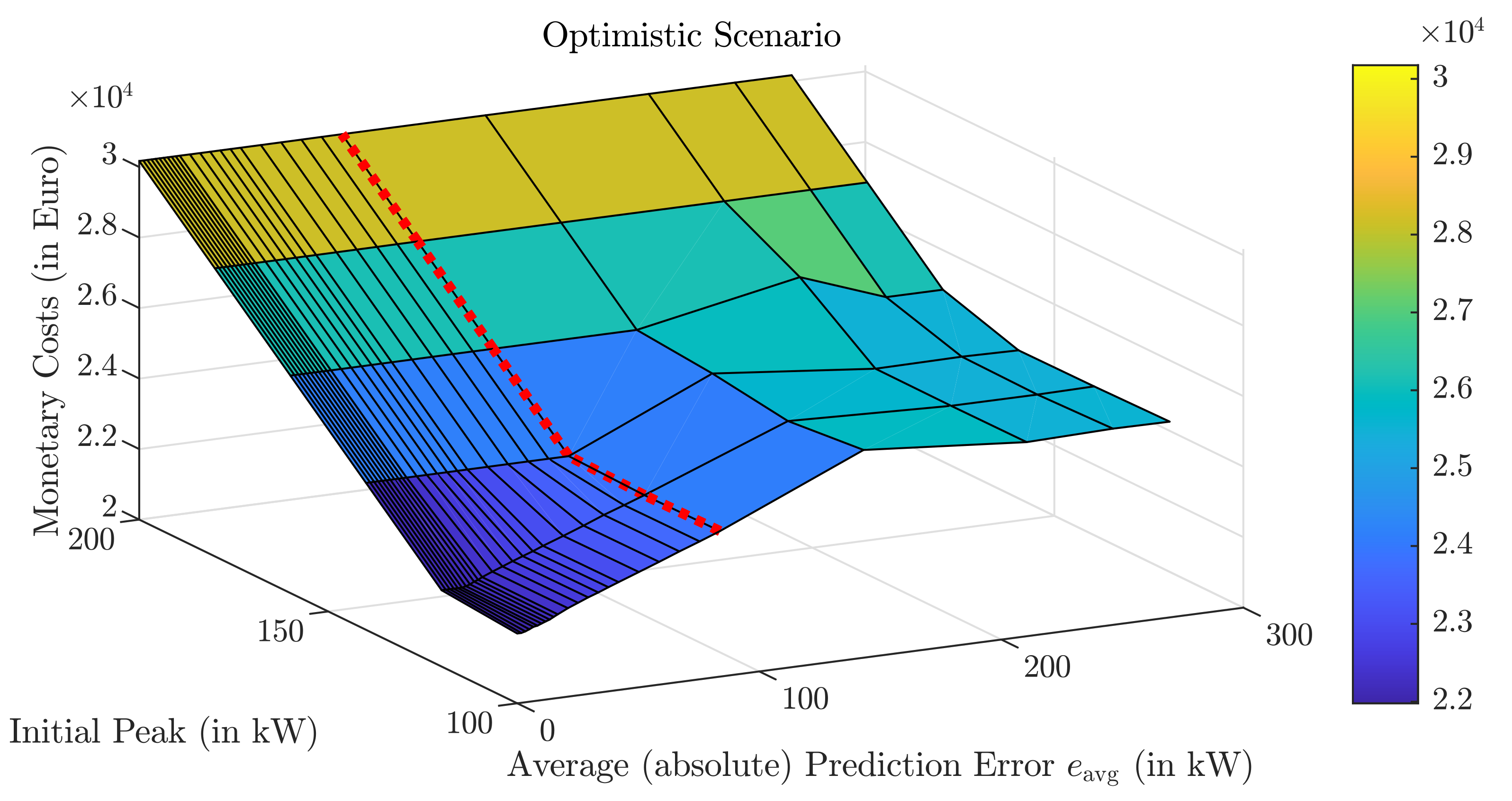
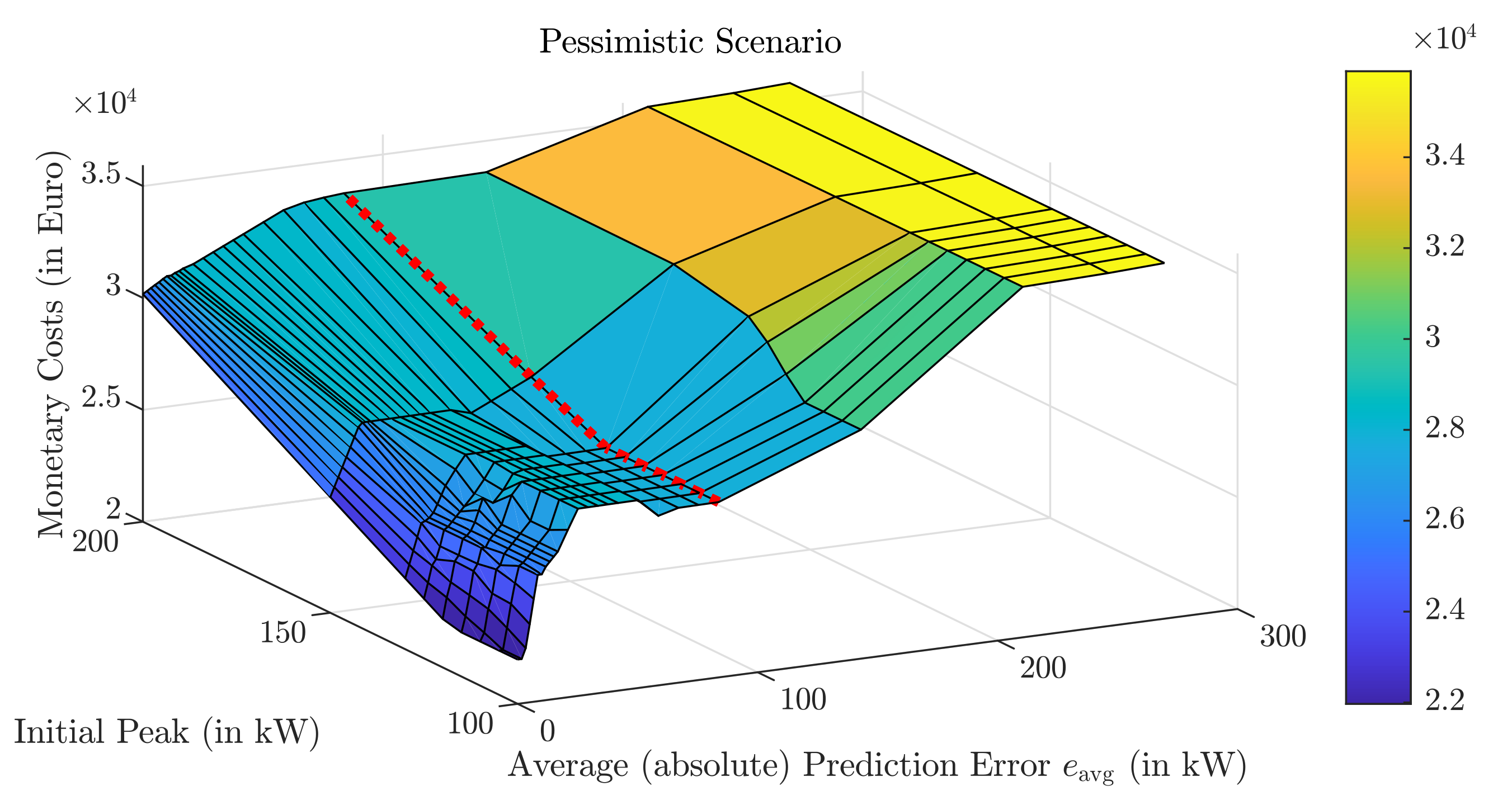
3.2. Correlation between Prediction Accuracy and Costs

To systematically analyze the correlation between prediction accuracy and resulting costs, we run multiple simulations with different initial peaks $P_{\mathrm{grid},\mathrm{peak}}\left(0\right)\in [100,200]\mathrm{kW}$ and vary $s_{\mathrm{err}}\in [0,8]$, leading to $e_{\mathrm{avg}}\in [0,269.6]\mathrm{kW}$, as described by (13). Figure 6 shows the results for the optimistic scenario.

With no prediction errors, the costs rise only with the initial peak costs (if ≥118 kW, which is unavoidable, see Figure 2). For low initial peaks ($100\mathrm{kW}$ or $120\mathrm{kW}$), the costs increase linearly with $e_{\mathrm{avg}}$ until ≈143.1 kW, from which point they start to saturate. For high initial peaks, $e_{\mathrm{avg}}$ has no influence on the costs, since $P_{\mathrm{grid},\mathrm{peak}}\left(0\right)+P_{\mathrm{chp}}^{\max }\ge -\left(P_{\mathrm{dem}}\left(k\right)+P_{\mathrm{ren}}\left(k\right)\right)\forall k$, and thus it is not necessary to use the battery for peak shaving.

Figure 7 shows the results for the pessimistic scenario. Here, the correlation is much less consistent and could be described by piece-wise linear functions for the different initial peaks. For lower initial peaks, the cost increases drastically for $e_{\mathrm{avg}}>0$. The higher the initial peak, the lower the slope becomes. However, in contrast to the optimistic scenario, costs do increase, even for the highest initial peak of $200\mathrm{kW}$. From $e_{\mathrm{avg}}\approx 25\mathrm{kW}$, the costs plateau (with one negative bump) and increase again with $e_{\mathrm{avg}}(s_{\mathrm{err}}>1)$.

The negative bump, i.e., the decrease in costs with an increased average error, can be explained by an artifact of the underlying data and would change, e.g., for other simulation time spans. To illustrate this, assume two simulations with $s_{\mathrm{err}}=0.5$ and $s_{\mathrm{err}}=1$. Usually, $s_{\mathrm{err}}=1$ will lead to higher peaks, e.g., at time step $k_1$. However, for a new demand peak at $k_2>k_1$, the controller 1 with $s_{\mathrm{err}}=0.5$ would thus try to shave the peak by discharging the battery, whereas controller 2 with $s_{\mathrm{err}}=1$ would not. If then, at $k_2+1$, an even higher peak occurs (previously unseen), controller 2 is in a better position and controller 1 might result in an overall higher peak. To conclude, luckily chosen higher prediction errors might lead to lower costs, but the general trend of increasing costs with higher errors is clear. Furthermore, the closer the error gets to 0, the more beneficial it seems, due to the high impact of peak costs, as Figure 8 shows.

3.3. Influence of Prediction Accuracy within the Time Horizon

For the simulations shown in Figure 6 and Figure 7, the prediction error werescaled equally over the prediction horizon as described in (12). To analyze whether its influence is equal over the horizon, too, we simulate with perfect predictions for the first $n_{\mathrm{perf}}$ steps. Figure 9 shows the resulting additional costs compared to a simulation with perfect overall predictions.

Note that $n_{\mathrm{perf}}=1$ for the optimistic and $n_{\mathrm{perf}}=0$ for the pessimistic scenario refer to the regular simulations (with real predictions). Furthermore, the pessimistic scenario with $n_{\mathrm{perf}}=1$ is the same as the regular optimistic scenario. In both scenarios, all additional costs are already avoided with $n_{\mathrm{perf}}=5$, i.e., with perfect predictions for the first $75\min$. Note that this is significantly shorter than a complete charging and discharging cycle of the stationary battery, which would take $250\min$.

4. Conclusions

We apply economic MPC to control a microgrid model of a medium-sized company building with real-world data from a 30-day period. Commercial weather forecasts are used for predictions of the power output of a PV plant. By linearly scaling the prediction error, we analyze the correlation between the average prediction error $e_{\mathrm{avg}}$ and the resulting monetary costs if peak costs apply, such as in the German industry pricing. Hereby, we make a distinction with regard to how prediction errors at the current time step are handled. First, we assume perfect knowledge (measurement) of the current power output, which, on average, would need to be the same over the next $15\min$ (referred to as the optimistic scenario). Second, we assume no additional measurement but the use of previously made forecasts (up to $65\min$ old), and compensate for errors in the power production by heuristic rules (referred to as the pessimistic scenario).

For both scenarios, the increase in monetary costs is mostly linear (optimistic), or at least peace-wise linear (pessimistic). Current weather forecasts can already be successfully utilized in an economic MPC, but further improvements would be rewarding. Moreover, simulations show that, for the presented setting, the prediction accuracy of only the first $75\min$ is relevant. Note that, most likely, this depends on the dynamics of the microgrid model. For example, this timespan might increase if minimal up and down times for combustion engines or other producers apply. Nevertheless, the employment of technologies for short-term predictions, such as sky cameras to monitor local cloud movements, seems promising. With these methods, real-world applications would shift towards our optimistic scenario, since the average value for the first $15\min$ could be predicted more reliably.

References

1. Bayer, F.A.; Müller, M.A.; Allgöwer, F. Tube-based robust economic model predictive control. J. Process Control 2014, 24, 1237–1246. [Google Scholar] [CrossRef]
2. Lucia, S.; Andersson, J.A.; Brandt, H.; Diehl, M.; Engell, S. I removed the ‘Informed Consent Statement’ since it does not apply: A comparative case study. J. Process Control 2014, 24, 1247–1259. [Google Scholar] [CrossRef]
3. Mayne, D. Robust and Stochastic MPC: Are We Going In The Right Direction? In Proceedings of the 5th IFAC Conference on Nonlinear Model Predictive Control NMPC 2015, Seville, Spain, 17-20 Sep 2015. IFAC-PapersOnLine 2015, 48, 1–8. [Google Scholar] [CrossRef]
4. Mesbah, A. Stochastic Model Predictive Control: An Overview and Perspectives for Future Research. IEEE Control Syst. Mag. 2016, 36, 30–44. [Google Scholar] [CrossRef] [Green Version]
5. Heirung, T.A.N.; Paulson, J.A.; O’Leary, J.; Mesbah, A. Stochastic model predictive control—How does it work? Comput. Chem. Eng. 2018, 114, 158–170. [Google Scholar] [CrossRef]
6. Cigler, J.; Prívara, S.; Váňa, Z.; Žáčeková, E.; Ferkl, L. Optimization of predicted mean vote index within model predictive control framework: Computationally tractable solution. Energy Build. 2012, 52, 39–49. [Google Scholar] [CrossRef]
7. Zia, M.F.; Elbouchikhi, E.; Benbouzid, M. Microgrids energy management systems: A critical review on methods, solutions, and prospects. Appl. Energy 2018, 222, 1033–1055. [Google Scholar] [CrossRef]
8. Zheng, Q.P.; Wang, J.; Liu, A.L. Stochastic Optimization for Unit Commitment—A Review. IEEE Trans. Power Syst. 2015, 30, 1913–1924. [Google Scholar] [CrossRef]
9. Lazos, D.; Sproul, A.B.; Kay, M. Optimisation of energy management in commercial buildings with weather forecasting inputs: A review. Renew. Sustain. Energy Rev. 2014, 39, 587–603. [Google Scholar] [CrossRef]
10. Agüera-Pérez, A.; Palomares-Salas, J.C.; González de la Rosa, J.J.; Florencias-Oliveros, O. Weather forecasts for microgrid energy management: Review, discussion and recommendations. Appl. Energy 2018, 228, 265–278. [Google Scholar] [CrossRef]
11. Oldewurtel, F.; Parisio, A.; Jones, C.N.; Gyalistras, D.; Gwerder, M.; Stauch, V.; Lehmann, B.; Morari, M. Use of model predictive control and weather forecasts for energy efficient building climate control. Energy Build. 2012, 45, 15–27. [Google Scholar] [CrossRef] [Green Version]
12. Lenzi, V.; Ulbig, A.; Andersson, G. Impacts of forecast accuracy on grid integration of renewable energy sources. In Proceedings of the 2013 IEEE Grenoble Conference, Grenoble, France, 16–20 June 2013; pp. 1–6. [Google Scholar] [CrossRef]
13. Romero-Quete, D.; Cañizares, C.A. An Affine Arithmetic-Based Energy Management System for Isolated Microgrids. IEEE Trans. Smart Grid 2019, 10, 2989–2998. [Google Scholar] [CrossRef]
14. Zhang, Y.; Wang, R.; Zhang, T.; Liu, Y.; Guo, B. Model predictive control-based operation management for a residential microgrid with considering forecast uncertainties and demand response strategies. IET Gener. Transm. Distrib. 2016, 10, 2367–2378. [Google Scholar] [CrossRef]
15. Khodaei, A.; Bahramirad, S.; Shahidehpour, M. Microgrid Planning Under Uncertainty. IEEE Trans. Power Syst. 2015, 30, 2417–2425. [Google Scholar] [CrossRef]
16. Mazzola, S.; Vergara, C.; Astolfi, M.; Li, V.; Perez-Arriaga, I.; Macchi, E. Assessing the value of forecast-based dispatch in the operation of off-grid rural microgrids. Renew. Energy 2017, 108, 116–125. [Google Scholar] [CrossRef]
17. Zhang, Y.; Liu, B.; Zhang, T.; Guo, B. An intelligent control strategy of battery energy storage system for microgrid energy management under forecast uncertainties. Int. J. Electrochem. Sci. 2014, 9, 4190–4204. [Google Scholar]
18. Hosseinzadeh, M.; Salmasi, F.R. Robust Optimal Power Management System for a Hybrid AC/DC Micro-Grid. IEEE Trans. Sustain. Energy 2015, 6, 675–687. [Google Scholar] [CrossRef]
19. Bertsimas, D.; Sim, M. The price of robustness. Oper. Res. 2004, 52, 35–53. [Google Scholar] [CrossRef]
20. Zhang, Y.; Gatsis, N.; Giannakis, G.B. Robust Energy Management for Microgrids With High-Penetration Renewables. IEEE Trans. Sustain. Energy 2013, 4, 944–953. [Google Scholar] [CrossRef] [Green Version]
21. Maasoumy, M.; Sangiovanni-Vincentelli, A. Optimal control of buildingHVAC systems in the presence of imperfect predictions. In Proceedings of the Dynamic Systems and Control Conference, Fort Lauderdale, FL, USA, 17–20 October 2012; American Society of Mechanical Engineers: New York, NY, USA, 2012; Volume 45301, pp. 257–266. [Google Scholar]
22. Maasoumy, M.; Razmara, M.; Shahbakhti, M.; Vincentelli, A.S. Handling model uncertainty in model predictive control for energy efficient buildings. Energy Build. 2014, 77, 377–392. [Google Scholar] [CrossRef] [Green Version]
23. Yang, S.; Wan, M.P.; Chen, W.; Ng, B.F.; Zhai, D. An adaptive robust model predictive control for indoor climate optimization and uncertainties handling in buildings. Build. Environ. 2019, 163, 106326. [Google Scholar] [CrossRef]
24. Ma, Y.; Matuško, J.; Borrelli, F. Stochastic Model Predictive Control for Building HVAC Systems: Complexity and Conservatism. IEEE Trans. Control Syst. Technol. 2015, 23, 101–116. [Google Scholar] [CrossRef]
25. Garifi, K.; Baker, K.; Touri, B.; Christensen, D. Stochastic Model Predictive Control for Demand Response in a Home Energy Management System. In Proceedings of the 2018 IEEE Power Energy Society General Meeting (PESGM), Portland, OR, USA, 5–10 August 2018; pp. 1–5. [Google Scholar] [CrossRef]
26. Schmitt, T.; Rodemann, T.; Adamy, J. Multi-objective model predictive control for microgrids. at-Automatisierungstechnik 2020, 68, 687–702. [Google Scholar] [CrossRef]
27. Schmitt, T.; Engel, J.; Rodemann, T.; Adamy, J. Application of Pareto Optimization in an Economic Model Predictive Controlled Microgrid. In Proceedings of the 28th Mediterranean Conference on Control and Automation, MED’20, Saint-Raphaël, France, 15–18 September 2020; Available online: https://tuprints.ulb.tu-darmstadt.de/11706/7/main_paper_pareto_FINAL%20VERSION_WITHLICENSEINFO.pdf (accessed on 9 May 2020).
28. Skoplaki, E.; Palyvos, J. On the temperature dependence of photovoltaic module electrical performance: A review of efficiency/power correlations. Sol. Energy 2009, 83, 614–624. [Google Scholar] [CrossRef]
29. Schmitt, T.; Engel, J.; Hoffmann, M.; Rodemann, T. PARODIS: One MPC Framework to control them all. In Proceedings of the 2021 IEEE Conference on Control Technology and Applications (CCTA), San Diego, CA, USA, 8–11 August 2021. in press. [Google Scholar]
30. Löfberg, J. YALMIP: A Toolbox for Modeling and Optimization in MATLAB. In Proceedings of the CACSD Conference, Taipei, Taiwan, 2–4 September 2004. [Google Scholar]
Figure 1. Illustration of the microgrid’s components.
Energies 14 02569 g001
Figure 2. Effective power demand, i.e., building consumption and PV production summed for the simulated time horizon. The black line shows the limit above which the CHP is insufficient to maintain a peak of 100 kW . The red line shows the limit if the battery is discharged at its maximum, i.e., the theoretic demand limit for which the initial peak of 100 kW could be held. On 11 May, a minimum peak of P grid 118 kW is unavoidable, even if the CHP and the battery are employed at their maximum.
Energies 14 02569 g002
Figure 3. Exemplary forecasts (blue lines) and measurement (black line) of solar irradiance for two days in April 2020. For a sunny day (Apr. 27), the forecasts do not change significantly over time and are reasonably accurate, apart from a small delay. For a cloudy day (Apr. 28), the day-ahead forecasts smoothen the variations in I sol . The closer a forecast is, the better it resembles the ups and downs. However, even with only 2 h ahead, the prediction error is still significant.
Energies 14 02569 g003
Figure 4. Exemplary comparison of true solar irradiance (black line) and most recent predictions available at the beginning of a time step (blue line) for 5 days. Besides forecasts being up to 65 min old, significant differences may occur due to the local distance between the site and the next weather station used for forecasting.
Energies 14 02569 g004
Figure 5. Monetary costs for simulations with perfect, real or no predictions. The initial peak was set to 100 kW (for which peak costs are included). The pessimistic scenario shows overall higher costs if prediction errors are present. (a) Optimistic Scenario; (b) Pessimistic Scenario.
Energies 14 02569 g005
Figure 6. Monetary costs for different prediction errors and initial peaks in the optimistic scenario. Peak costs of the initial peaks are included. The red dotted line shows the error level with real predictions ( e avg ( s err = 1 ) = 83.76 kW ).
Energies 14 02569 g006
Figure 7. Monetary costs for different prediction errors and initial peaks in the pessimistic scenario. Peak costs of the initial peaks are included. The red dotted line shows the error level with real predictions ( e avg ( s err = 1 ) = 83.76 kW ).
Energies 14 02569 g007
Figure 8. Parts of the additional monetary cost which are not caused by higher peaks. Again, the red lines indicate the real average prediction error. For the optimistic scenario (a), only simulations with initial peaks of 100 kW or 120 kW are shown, since, with higher initial peaks, generally, no new peaks occur. For lower initial peaks, they dominate, i.e, the non-peak costs are negligible (≤2%). For the pessimistic scenario (b), the part of additional non-peak costs increases with both higher e avg and initial peaks in P grid . However, in the most relevant part with initial peaks 120 kW , they are still low (≤5%). (a) Optimistic Scenario; (b) Pessimistic Scenario.
Energies 14 02569 g008
Figure 9. Additional costs in comparison to perfect simulation when the first n perf steps of the prediction horizon are perfectly predicted. For both scenarios, additional costs are avoided for n perf 5 . (a) Optimistic Scenario; (b) Pessimistic Scenario.
Energies 14 02569 g009