Article

Application of an Artificial Neural Network for Measurements of Synchrophasor Indicators in the Power System

Institute of Electrical Power Engineering, Lodz University of Technology, Stefanowskiego 18/22, 90-924 Lodz, Poland
*
Author to whom correspondence should be addressed.
Energies 2021, 14(9), 2570; https://doi.org/10.3390/en14092570
Submission received: 23 March 2021 / Revised: 21 April 2021 / Accepted: 26 April 2021 / Published: 30 April 2021
(This article belongs to the Special Issue Electromagnetic Energy in Modern Engineering and Medical Technologies)

Abstract

:
Dynamic phenomena in electric power systems require fast and accurate algorithms for processing signals. The processing results include synchrophasor parameters, e.g., varying amplitude, phase or frequency of sinusoidal voltage or current signals. This paper presents a novel estimation method of synchrophasor parameters that comply with the requirements of IEEE/IEC standards. The authors analyzed an algorithm for measuring the phasor magnitude by means of a selected artificial neural network (ANN), an algorithm for estimating the phasor phase and frequency that makes use of the zero-crossing method. The original components of the presented approach are: the method of the synchrophasor magnitude estimation by means of a suitably trained and applied radial basic function (RBF); the idea of using two algorithms operating simultaneously to estimate the synchrophasor magnitude, phase and frequency that apply identical calculation methods are different in that the first one filters the input signal using the FIR filter and the second one operates without any filter; and the algorithm calculating corrections of the phase shift between the input and output signal and the algorithm calculating corrections of the magnitude estimation. The error results obtained from the applied algorithms were compared with those of the quadrature filter method and the ones presented in literature, as well as with the permissible values of the errors. In all cases, these results were lower than the permissible values and at least equal to the values found in the literature.

1. Introduction

Changes taking place in modern electrical power systems require continuous and reliable monitoring of their working states, mainly due to the need to provide electrical power safety. In recent years, there has been a significant increase in electrical energy generation by renewable energy sources. This entails the development of connected electrical power systems driven by the increase in demand for electrical energy, as well as by adding new elements to the already-existing electrical power systems. From the other side, the optimization of operating conditions of entire electrical power systems and their elements approaches their limit values. In modern networks, this problem is commonly carried out by the wide area measurement system (WAMS), which consists of measurement devices called phasor measurement units (PMUs) located in selected points of an electrical power system; mainly in the substation bays [1]. PMUs measure instantaneous current or voltage values, calculating their parameters: the phasor magnitude, angle and frequency, and the rate of change of frequency (ROCOF). The phasor angle is calculated in relation to the coordinate system that rotates with the electrical power system’s nominal frequency. PMU results are marked with Global Positioning System (GPS) timestamps converted to Coordinated Universal Time (UTC), and are called synchronous measurements. The synchronization error results from a GPS accuracy of around 1 µs, which is equivalent to 0.018° or 0.0314 rad angle error. This, in turn, generates a calculation error of approximately 0.03% [2,3,4].
In the WAMS system, it is necessary to consider the selection of PMU installation locations, and therefore also the selection of their number; to determine the optimal structure of the WAMS system, including information transmission methods; to determine the algorithm for converting instantaneous current or voltage values into estimated parameters (phasor amplitude and angle, frequency and ROCOF); and to define the way of using the obtained synchrophasor parameters to determine the operating state of the power system. The definition of the parameters to be met by PMU devices is included in the IEEE standards [2,3,4].
In the literature, many publications may be found regarding the estimation methods of the synchrophasor magnitude, angle and frequency, as well as calculating the synchrophasor errors defined in standards [2,3,4]. Fourier transform (FT) [5] and its variations [6,7,8,9,10,11,12,13,14] are the most popular methods used to measure the signal magnitude and angle, since they are efficient and mostly reliable. In turn, the quadrature filter method is based on the multiplication of the input signal by two sinusoidal orthogonal functions with the nominal frequency [15,16,17]. The phase lock loop (PLL) method contains a feedback loop within the PID [18] regulator that is responsible for resetting the phase difference between the input and output signal. The least squares method (LSM) uses the unknown parameters of measurement values for estimation, and identifies them using the smallest mean-square error [12]. Many other estimation methods can be found in the literature; e.g., Kalman’s filter [19,20,21,22,23], which is particularly recommended when a signal includes stochastic interference; the continuous wavelet transform (CWT) method, which is used for calculating phasor parameters [24]; Prony’s method, in which the analyzed signal is replaced with exponentially damped sinusoids in order to minimize the mean-square error [25]; the four parameters (4P) algorithm, which verifies the real part of the Taylor series of the analyzed phasor and has four basic parameters [26,27,28]; and the six parameters (6P) method [27]. Artificial neural networks (ANNs) are used in many computational problems of electrical power systems [29,30,31]. In [32], the authors described the use of a radial basic function (RBF) of an ANN to calculate signal frequency by means of minimizing the entire phasor error; and in [33], to calculate the synchrophasor parameters. In [34,35], the authors used ANNs to identify phasor parameters, while in [36], ANNs were used to calculate the synchrophasor parameters only by considering the static functions.
From the above, it is seen that the publications lack a complete testing process of a given method in which all the reference test signals in compliance with IEEE standards are used [2,3,4]. This article deals with the issue of application of an artificial neural network to measure the synchrophasor’s parameters in static and dynamic power systems. ANN is a new, more accurate algorithm for converting the instantaneous current or voltage values into the synchrophasor parameters (the phasor magnitude, angle and frequency) for the P and M classes of PMU devices. Additionally, the paper presents the requirements that must be met by estimation methods of phasor parameters, including the method of estimating phasor errors and their permissible values, as well as a flowchart of a new estimation method used for phasor parameters. The authors’ method proposes the following measurement algorithms: the phasor magnitude calculated using a radial ANN, the phasor phase and frequency calculations using the zero-crossing method. The error values obtained from the flowchart were compared with the results of the quadrature filter method (as was recommended and described in standards [2,3,4]), with the results presented in the literature as well as with the phasor permissible error values provided in standards [2,3,4]. The RBF of the ANN used in this article is characterized by the speed and accuracy in terms of the results obtained, which is an important issue when researching the dynamic states of an electrodynamic system, in particular when overvoltage or other system failures occur. In a novel approach, it uses two simultaneously operating algorithms that may estimate the synchrophasor magnitude, phase and frequency. These algorithms apply identical calculation methods, but they differ from each other in that the first one filters the input signal using the FIR filter, while the second one operates without any filter. The approach allows for calculating the corrections of the phase shift between the input and output signal and the corrections of the magnitude estimation. In addition, the algorithms propose estimation of phasor magnitude using functions including out-of-band interference, which are the most difficult functions for magnitude estimation.
The organization of the paper is as follows. Section 2 presents the requirements imposed on the estimation methods of phasor parameters of the signal model used, a new algorithm for measuring the phasor magnitude by means of a radial artificial neural network and an algorithm for estimating the phasor phase and frequency that makes use of the zero-crossing method. Numerical results for the P and M classes are shown in Section 3, together with discussion of the results obtained. The conclusions from the studies are given in Section 4.

2. Methodology of the Studies

2.1. The Requirements Imposed on the Estimation Methods of Phasor Parameters

The continuous and periodic sinusoidal signal of current or voltage can be presented as a phasor; i.e., a vector rotating in the coordinate system that rotates with the electrical power system’s nominal frequency. In addition, standards specify the notion of a synchrophasor; i.e., a phasor that marks every analyzed sample with a UTC timestamp [2,3,4].
Standards provide 10 types of testing functions for PMU devices of the P (protection) and M (measurement) classes. Class P is used in protection that requires a quick response and allows for less precise measurements when the fundamental wave of the signal has a frequency other than 50 Hz. On the other hand, the M class is used when the measurement accuracy is the most important, and the possibility of a longer delay than for the P class is acceptable. Different courses of the testing functions have been defined for each of the classes. These functions listed below are divided into two types of signals: static (1–5) and dynamic (6–10):
  • The sinusoidal function with a constant magnitude of 1 and a constant frequency of 50 Hz (denoted as function 1);
  • Functions with a constant frequency of 50 ± 2 Hz for the P class and of 50 ± 5 Hz for the M class (denoted as functions 2 and 3);
  • Functions with a magnitude change between 0.1 and 2. The authors assumed the values of 0.1, 0.8, 1.2 and 2 (denoted as functions 4, 5, 6 and 7, respectively);
  • Functions including the harmonics from the 2nd to the 50th with a magnitude of 0.01 for the P class and 0.1 for the M class (denoted as functions from 8 to 56);
  • Functions including out-of-band interference. These exist only in the M class and have a magnitude of 0.1. The input test signal frequencies are as follows:
  • f = f0 − (FS/2) − (0.1 Hz × 2n) for n = 0, 1, 2, … to f ≤ 10 Hz for n = 0, 1, 2, … to f ≤ 10 Hz; i.e., they include the following frequency values: 12.2, 18.6, 21.8, 23.4, 24.2, 24.6, 24.8 and 24.9 Hz (denoted as functions from 57 to 64);
  • f = f0 + (FS/2) + (0.1 Hz × 2n) for n = 0, 1, 2, … to f ≥ 2 × f0 Hz; i.e., they include the following frequency values: 75.1, 75.2, 75.4, 75.8, 76.6, 78.2, 81.4 and 87.8 Hz (denoted as functions from 65 to 72);
  • Where FS—the reporting frequency—is assumed to be 50 samples/s. Assuming the reporting frequency to be 50 samples/s means that the estimated synchrophasor parameters should be obtained from the signal of the maximum length of 0.02 s, irrespective of the network frequency;
6
Functions with a magnitude modulation, where the signal is a sum of the base signal and the sinusoidal signal of a magnitude of 0.1 and the frequency changes between 0.1 and 2 Hz for the P class and between 0.1 and 5 Hz for the M class, with a change occurring every 0.1 Hz (denoted as functions 57 to 76 for the P class and functions 73 to 122 for the M class);
7
Functions with a phase modulation, where the base signal phase additionally contains the sinusoidal signal with a magnitude of 0.1 rad and the frequency changing between 0.1 and 2 Hz for the P class and between 0.1 and 5 Hz for the M class, with a change occurring every 0.1 Hz (denoted as functions 77 to 96 for the P class and functions 123 to 172 for the M class);
8
Functions with linear ramp of system frequency, where the ramp range is ±2 Hz for the P class and ±5 Hz for the M class, with a ramp rate of 1 Hz/s (denoted as functions 97 and 98 for the P class and functions 173 and 174 for the M class);
9
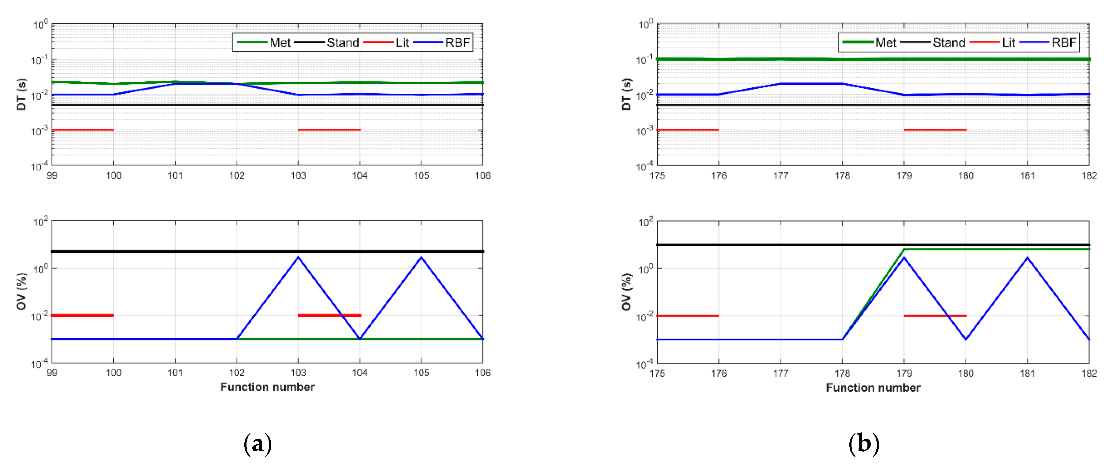
Functions with a step magnitude change of ±0.1 and with a step occurring at the beginning and in the middle of the measurement window (denoted as functions 99 to 102 for the P class and functions 175 to 178 for the M class); the functions having a step occurring in the middle of the measurement window are additional testing functions implemented by authors for research measurements;
10
Functions with a step phase change of ±π/10 and with a step occurring at the beginning and in the middle of the measurement window (denoted as functions 103 to 106 for the P class and functions 179 to 182 for the M class).
The errors that must be estimated by the PMU devices are described in the IEEE standards [2,3,4]. They are valid for all the testing functions, except step functions of total vector error (TVE), which is a Euclidean vector space of the difference between the measured synchrophasor and the reference synchrophasor, both at the same time. Frequency error (FE) is given as the difference between the measured and the reference frequencies. In turn, the rate of change of frequency error (RFE) is the difference between the measured rate-of-change of frequency and the reference rate-of-change of frequency, both at the same time.
Errors for step functions include:
  • Response time of TVE (RT-TVE), which means a time difference between the point at which the TVE value decreases below 1% and the point at which the TVE increases above 1%;
  • Response time of FE (RT-FE) which means a time difference as defined in point 4 but for the FE value of 0.005 Hz;
  • Response time of RFE (RT-RFE), which means a time difference as defined in point 4 but for the RFE value of 0.4 Hz/s for the P class and 0.1 Hz/s for the M class;
  • Delay time (DT), which is a time difference between the point at which the magnitude or phase reach 50% of the step value and the initial step value;
  • Overshoot/undershoot value (OV), which is a difference between the maximum magnitude or phase value following a step and the step value, which is further divided by the step value.
The permissible error values of synchrophasor parameters are provided in different sections of the analyzed standards and are collected in Table 1.
Testing each estimation method of synchrophasor parameters is conducted for the same signal composed of all the testing functions one by one. It is assumed that every testing function lasts 2 s (the 1st second aims to eliminate the transient state and during the 2nd second synchrophasor errors are estimated). The only exception are functions with linear ramp of system frequency: for frequency range of ±2 Hz and frequency rate of 1 Hz/s, the frequency changes (i.e., it increases or decreases) over 4 s. Therefore, a linear ramp testing function lasts 8 s in total. For frequency range of ±5 Hz and frequency rate of 1 Hz/s, the frequency changes (i.e., it increases or decreases) over 10 s. Therefore, a linear ramp testing function lasts 14 s in total. This testing method causes the total length of the testing function to be 228 s for the P class and 392 s for the M class.
The constant sampling frequency fp of the signal is equal to 12,800 Hz, which means L = 256 samples in one measurement window. This means that each measurement window lasts 0.02 s. It was decided that the end of one measurement window is the beginning of the next one, but another sequence is also possible; i.e., the next window overlaps the previous one.
For the quadrature filter method, the constant sampling frequency of the signal was assumed to be 12,750 Hz, which results from the method characteristics and is defined in the standards.

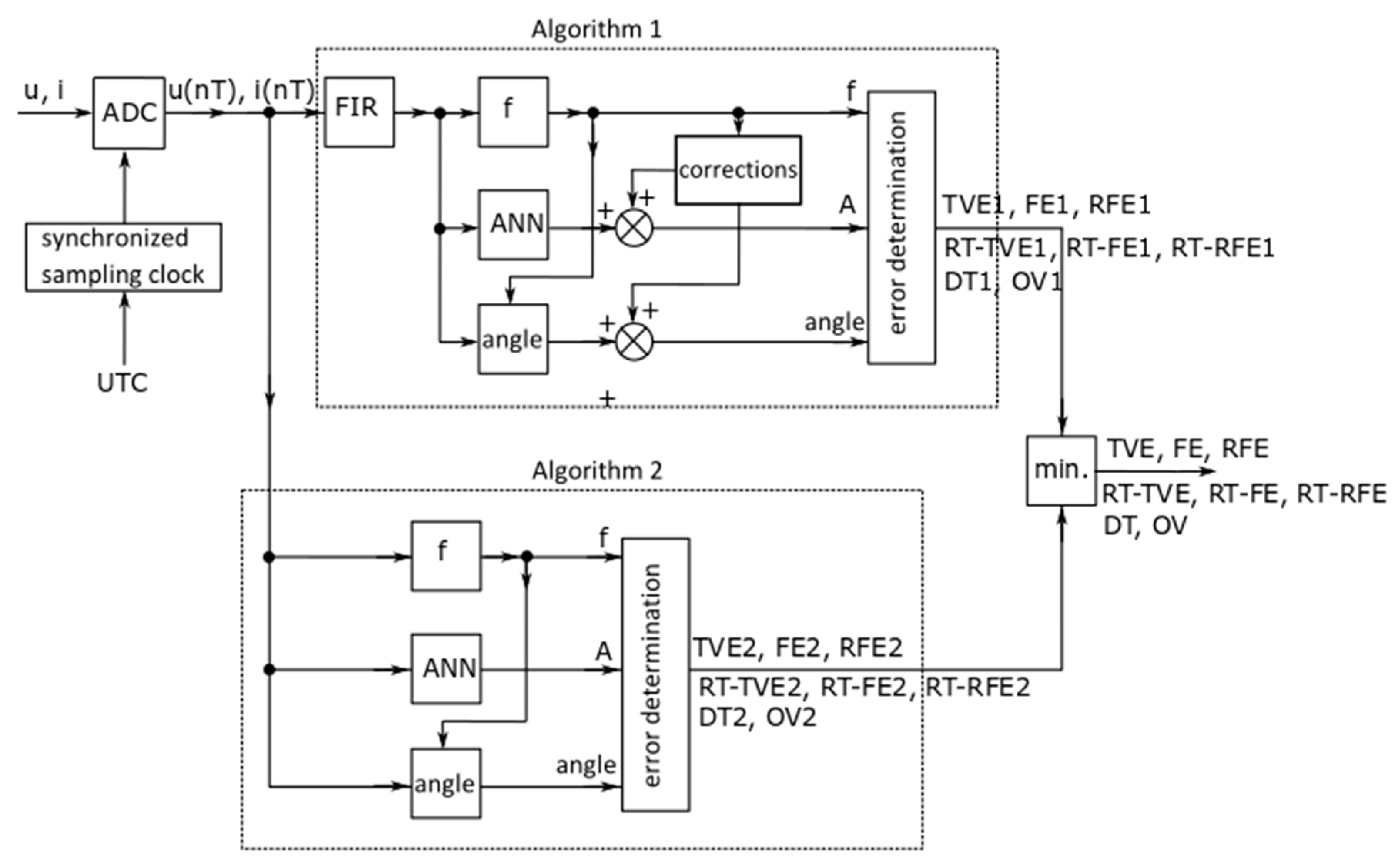
2.2. The Flowchart of the Estimation Algorithm of the Phasor Parameters

The paper proposes a new, more accurate algorithm for converting the instantaneous current or voltage values into the synchrophasor parameters (the phasor magnitude, angle and frequency) for the P and M classes of PMU devices and for the conditions defined in standards: test signal, the methods for calculating measurement errors of the synchrophasor parameters and the limit values of measurement errors of the synchrophasor parameters.
Testing the new algorithm for converting the instantaneous current or voltage values into the synchrophasor parameters was conducted by means of computer simulations using MATLAB software, and the aim was to calculate measurement errors and compare them with permissible errors (included in Table 1). The presented method made it possible to accurately calculate the synchrophasor magnitude, phase and frequency by means of two algorithms working simultaneously, and the final result was the smaller of the two values provided by the algorithms. Both algorithms used the identical calculation methods of the synchrophasor magnitude, phase and frequency, and the main difference was the fact that the first one filters the input signal by means of the finite impulse response (FIR) filter, and the second one operates without any filter. The most important features of the first algorithm are:
  • The filtering of the input signal was conducted by means of the FIR filter with a Kaiser window. The filter parameters were as follows: frequency of a passband edge of 50 Hz, frequency of a stopband edge of 100 Hz, passband ripple of 0.001 pu, stopband ripple of 0.1 pu, sampling frequency of fp = 12,800 Hz, order of 929 and Kaiser window beta of 5.6533.
  • The zero-crossing method was used to estimate the frequency and phase;
  • An RBF of the ANN was used to estimate the magnitude;
  • A frequency-dependent algorithm to make corrections to the estimation results of the magnitude and phase was used.
In the second algorithm, apart from the fact that no filter was used, the estimation of magnitude, phase and frequency was conducted in the same way as in the first algorithm. Here, due to the elimination of the filter, the application of the magnitude and phase correction algorithm was not required. The flowchart presenting the algorithm for converting instantaneous current or voltage values into the synchrophasor parameters is shown in Figure 1.
Figure 1 shows the following processes of the synchronized sampling clock: ADC—the analogue–digital converter; FIR—the low pass filter, f, and ANN and angle, for estimating the synchrophasor frequency, magnitude and phase, respectively; corrections—calculating corrections of the synchrophasor magnitude and phase; error determination—determination of the synchrophasor errors; min.—calculates the results the synchrophasor frequency, magnitude and phase errors selecting the smaller of the two input values; signals: u, i—the instantaneous voltage or current values; u(nT), i(nT)—the discrete voltage or current values; f, A, angle—the synchrophasor parameters: frequency, magnitude and phase; TVE, FE, RFE, RT-TVE, RT-FE, RT-RFE, DT, OV—the synchrophasor errors.

2.3. The Phasor Magnitude Estimation Algorithm Using ANN

Different ANNs were analyzed using MATLAB software during the pre-studies in order to identify the magnitude of any sinusoidal signal (for example, Elman neural network, radial basic function, linear neural network, back propagation neural network, regression neural network, multilayer perceptron or feedforward neural network). These analyses used the training process, which was based on assumptions that the input signal (training function) was the matrix 20 × 5, where 20 meant a number of changes of signal magnitude, while 5 meant an appropriate number of samples selected from the learning signal neighborhood. A sinusoidal signal with the following parameters was applied: a magnitude of 0.1 pu to 2.0 pu changing every 0.1 pu, a constant frequency of 50 Hz and a constant phase equal zero. The input layer was 1, the number of hidden neurons was 10 and the output layer was 1. From the considered networks, the RBF was solely chosen as the solution that successfully met all the requirements for the identification accuracy of the signal magnitude within the assumed range of frequency, phase and magnitude changes. This was due to the fact that for the RBF, the method error was obtained as the lowest, below 2.085 × 10⁻¹⁴. However, the results in the field of choosing the ANN type were omitted herein, as they were not directly related to the study’s objectives.
In general, the RBF consists of the input layer, the hidden layer and the output layer (responsible for the network response). The neurons are excited when they recognize the situation that they were taught. The advantage of the RBF is a quick learning process, good generalization of data and structural simplicity in comparison with other neural networks [37]. To estimate output weight vectors, it mainly uses the least squares method [38].
From the above, having trained the network for the assumed conditions, as well as the learning function, the tests were conducted and the sufficient accuracy of the trained network was obtained. Although the RBF was trained for fixed frequency and phase values, it correctly estimated the signal magnitudes for any magnitude, phase and frequency of the input signal. During operation, this method only required the same number of samples as during the learning process, selected from the learning signal neighborhood extreme of the analyzed function. The method used samples from the maximum half of each measurement window; i.e., 128 samples, and for signals of frequency smaller than 50 Hz, it simultaneously used 30 samples from the previous window.

2.4. The Synchrophasor Frequency and Phase Estimation Algorithm Using the Zero-Crossing Method

For the synchrophasor frequency estimation, the zero-crossing method was used, as it is one of the most frequently considered algorithms in terms of its calculation simplicity, accuracy and dynamism. In this method, three consecutive zero crossings are chosen from all samples. In order to increase accuracy, the zero-crossing point was calculated using linear interpolation. The synchrophasor estimated frequency fei in the ith measurement window was calculated using Equation (1) as follows:
fei = fp/(t2ei − t1ei)
where fp is the signal sampling frequency, t1ei is the sample with the first zero-crossing point of the input signal in the ith measurement window and t2ei is the sample with the third zero-crossing point of the initial signal.
The sampling frequency influences the frequency estimation accuracy of the analyzed function. The method’s advantage is its speed of frequency estimation, and its disadvantage is the sensitivity to signal distortions: high harmonics or interharmonics, etc. Therefore, the authors used the initial signal filtering by means of the FIR filter.
In order to estimate the signal phase in the first measurement window, the first zero-crossing point of the initial signal was used, and the estimated signal phase was calculated using Equation (2) as follows:
φe1 = (π/2) − (2 ∙ π ∙ t1e ∙ fei)/fp
In the subsequent measurement windows, phases were calculated according to Equation (3):
φei = φe (i − 1) + 2 ∙ π ∙ (fei/f0) − 2 ∙ π ∙(i − 1) for i = 2, 3, …, n
where: n is the total number of measurement windows.

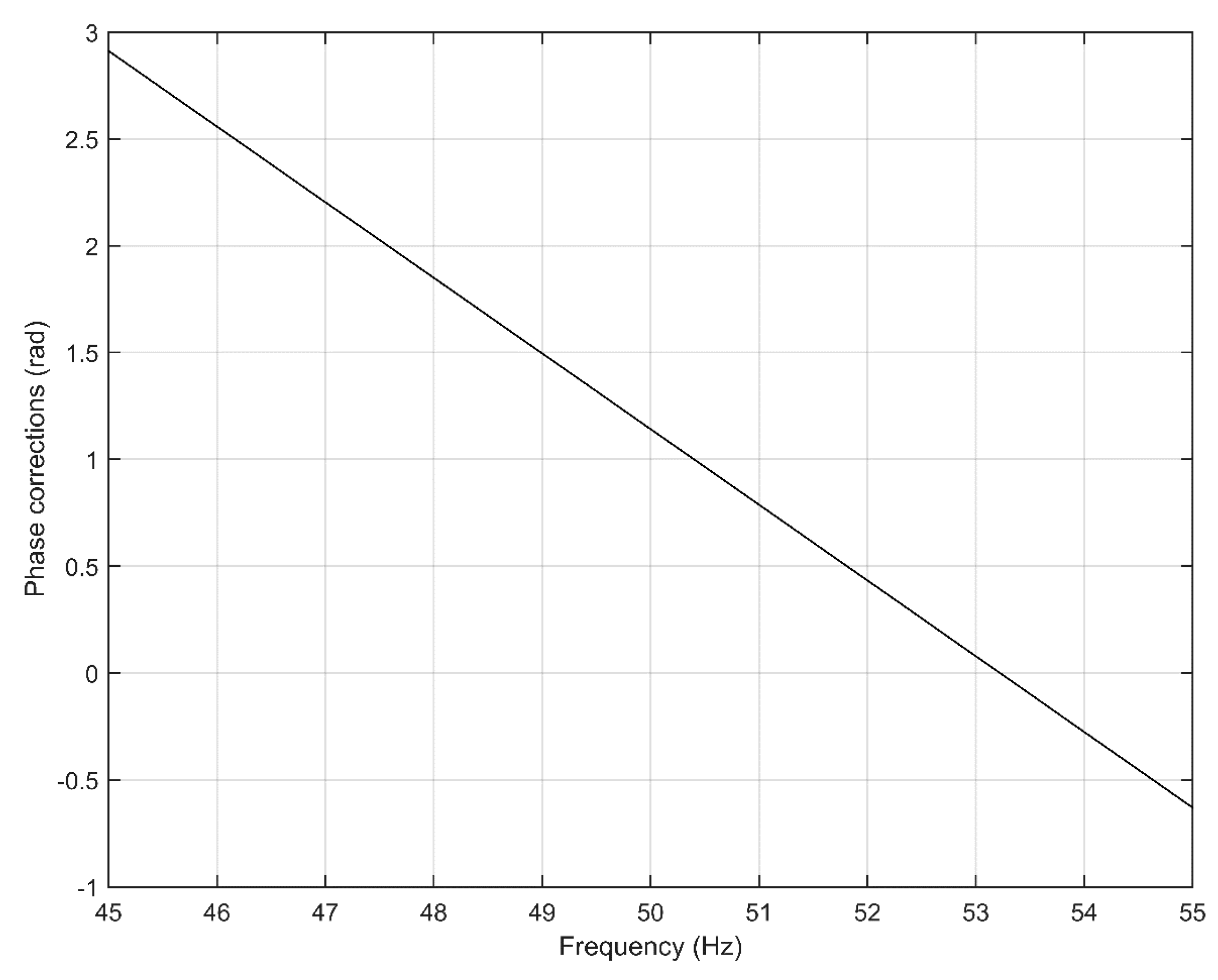
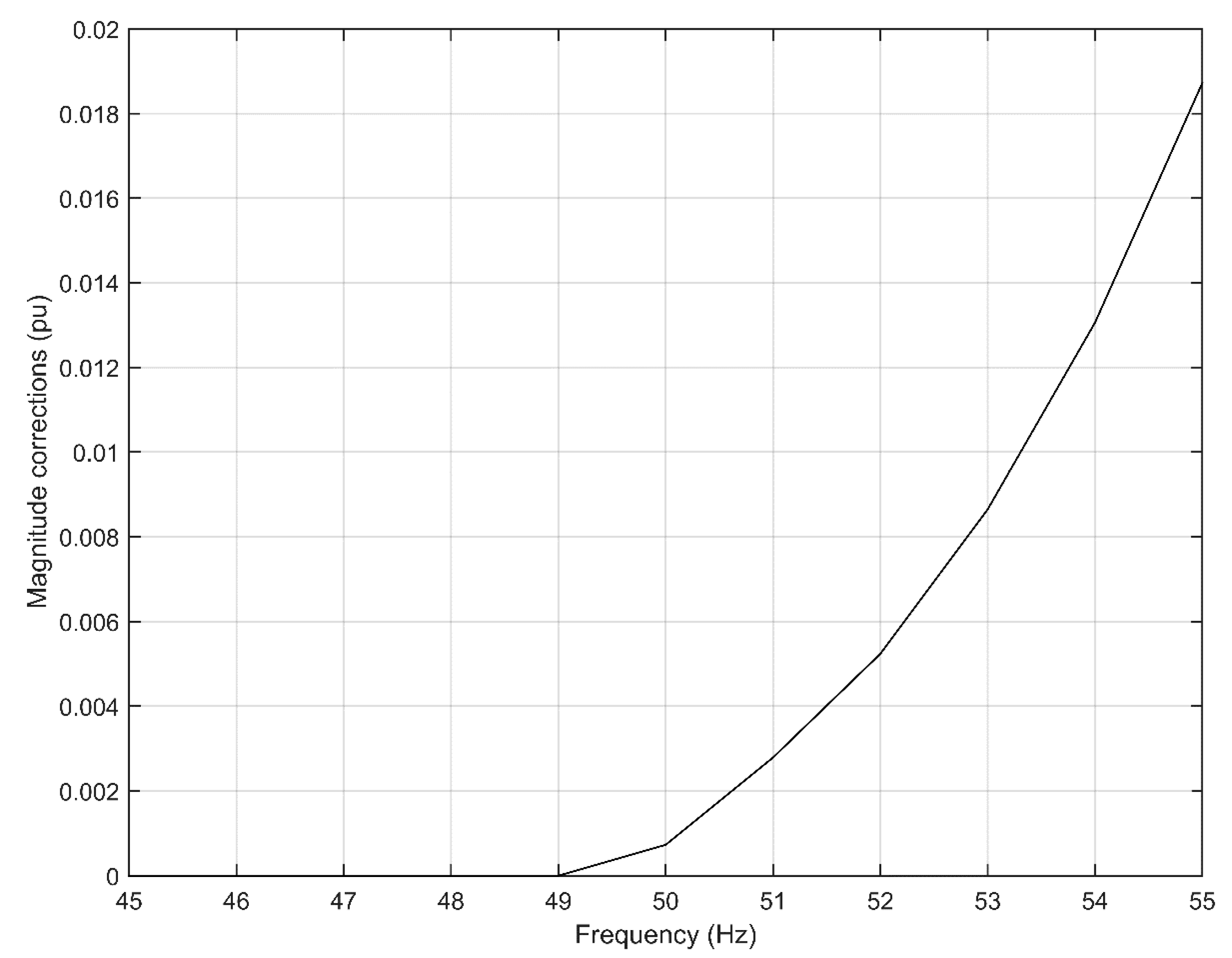
2.5. Corrections of the Synchrophasor Magnitude and Phase Estimation

The linear phase FIR filter was used in the presented research, and it was characterized by a constant group delay; i.e., the phase difference between the input and output signals depended linearly on the input-signal frequency. As a result, to compensate for the filter delay, the correction factor was applied to the estimated output signal phase (Figure 2) as in Equation (4):
Δϕe = −0.3542 ∙ fe + 18.85
A similar procedure was used for calculating the correction factors for the compensation of the magnitude estimation obtained as a result of using the RBF. To estimate the magnitude correction factors, a piecewise linear approximation was used with a step of 1 Hz. The calculation results are presented in Figure 3.

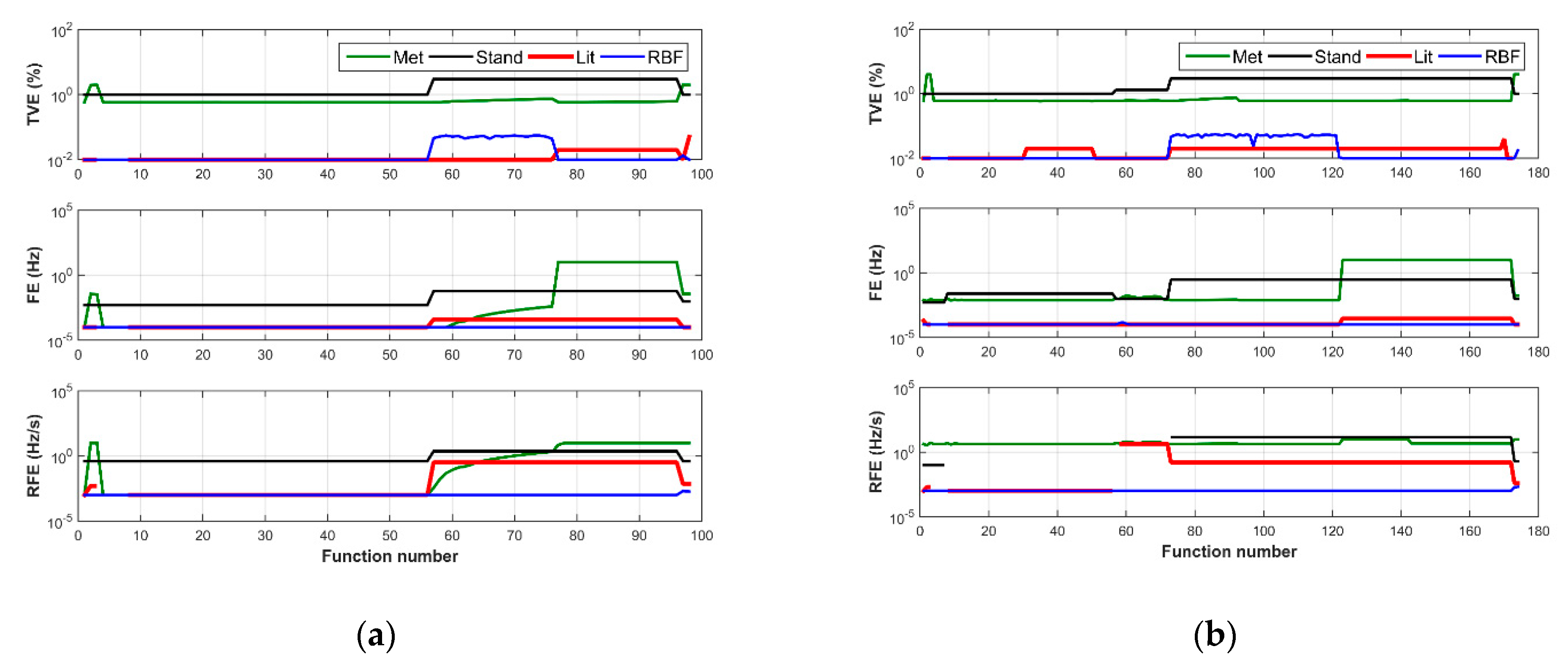
3. Results and Discussion

Figure 4, Figure 5, Figure 6 and Figure 7 present the error results of the RBF (marked as RBF—blue color), the quadrature filter method (marked as Met—green color), the permissible error values from standards (Stand—black color) and the results published in the literature [14,15,16,17,22,23,26,27,28,39,40,41] (Lit—red color), respectively, for the P class of the PMU device in part (a) of each figure and for the M class of the PMU device in part (b) of each figure. The comparative form of the results presentation was applied. From the figures, it may be stated that none of the results published in the literature represented the situation when the same method provided the data for all the testing functions. In some cases, the testing functions even lacked any results. It is commonly known that it is easy to obtain very good results for a selected group of testing functions. However, it is more difficult to do so for a wider range of functions.
As mentioned in Table 1 and visible in the quoted figures, 106 test functions in total were used for the P class PMU device, and 182 test functions in total for the M class PMU device. This difference in the number of functions resulted from the different values of modulation frequency, which for the P class was changed from 0.1 Hz to 2 Hz with a 0.1 Hz step, and for the M class from 0.1 Hz to 5 Hz with a 0.1 Hz step.
After analyzing the obtained error results presented in Figure 4 for the P and M classes, it can be stated that when using the authors’ method, the values of TVE, FE and RFE, which were tested using the functions from 1 to 98 for the P class and the functions from 1 to 174 for the M class, were always smaller than permissible values, the values obtained using the quadrature filter method and, in most cases, the results published in the literature. In the latter, due to the fact that the RBF method was very sensitive to the appearance of magnitude modulations (functions 57–76 for the P class and functions 73–122 for the M class), the TVE was on the level of circa 0.05% (slightly higher then literature data); however, for the rest of test functions it oscillated around the value of 0.01%. In contrast, the results concerning the quadrature filter method were 0.6%.
Similar observations to the above concerns also were seen in the results connected with the FE. The RBF-method-based results were comparable when comparing the P and M classes, and were around 0.0001 Hz. At the same time, the quadrature filter method for the functions with phase modulation (77–96 for P class and 123–172 for M class) gave results on the level of around 10 Hz, which exceeded the permissible values.
An analogous situation was noticed for the RFE. The results using the authors’ approach were equal to 0.001 Hz/s for both classes and the whole range of test functions, while for the quadrature filter method, the results were much higher (5 Hz/s for the P class and circa 9.5 Hz/s for the M class), when functions with a phase modulation were considered. For the same types of functions, the literature data also gave worse results for RFE than when the RBF method was applied.
In the case of the RT-TVE and RT-RFE values, the results were also promising for the applied authors’ method and for all testing functions. For the M class, the results were lower than other data for all functions applied. Exemplary, the highest values that were obtained for functions 181 and 182 (0.038 s) were lower than the permissible values and the quadrature filter method. The RT-TVE and RT-RFE values for the P class of the PMU device were slightly worse for some testing functions. However, the differences in relation to the quadrature filter method, as well as literature data, were not large.
In turn, after assessing the RT-FE values, we can state that they were smaller than the permissible values and the literature-based results for all testing step functions. Their values for testing functions with step changes in magnitude were also smaller than the results obtained using the quadrature filter method. However, for testing functions with step changes in phase, the results concerning RBF method were larger than the results obtained by means of the quadrature filter method. These values could be easily minimized by using a smaller step of the measurement window shift, but it would lengthen the calculation time.
In detail, the RT-FE and RT-RFE for both classes considered increased for the testing functions, with a step phase change of ±π/10 and with a step occurring at the beginning and in the middle of the measurement window. The obtained values were around 0.04 s (class P at testing functions from 103 to 106 and class M at testing functions from 179 to 182) for RT-FE, and 0.058 s for class P and 0.06 s for class M of RT-RFE.
When analyzing DT values, it was noticed that they were larger than permissible values, but smaller than the results obtained using the quadrature filter method, both in the case of the P and M classes of the PMU device. They could be minimized using the smaller step of the measurement window shift. DT values obtained using authors’ approach also were larger than the results provided by literature (only [41] presented such the values, and it did so just for some parts of the testing step functions). The OV errors were smaller than the permissible values and the results provided in the literature [22,23,39,40,41], and for the M class also were lower than those concerning the quadrature filter method.
The analyses were also focused on the magnitude errors defined as an absolute value of the difference between the magnitude obtained by means of the RBF and the input signal magnitude. These errors were close to zero, except the functions containing interharmonics (their values were around 0.005), and for the functions with a step phase change (their values were around 0.01). When analyzing the TVE, FE, RFE, RT-TVE, RT-FE, RT-RFE, DT and OV values, separately for class P and class M, the universality of this method could be noticed. Differences in requirements for the P and M classes were not a problem for the RBF method; this was confirmed by the fact that the results obtained were similar and did not exceed the permissible values (except for the DT time) specified in the standards.

4. Conclusions

The paper presents a method for synchrophasor magnitude, phase and frequency estimation using two algorithms working simultaneously, for which the final results, in terms of errors estimated, were smaller than for each individually. Both algorithms used identical calculation methods for the synchrophasor parameters. The main difference between them was that the first one used the FIR filter for the input signal, while the second one did not use any of the filters available. The synchrophasor parameters were estimated as follows: frequency—by applying the well-known zero-crossing method; phase in the first step—from the zero crossing in the first measurement window; phase in each of the subsequent windows—from the phase from the previous window and the frequency value from a given window; and magnitude—by means of the RBF. In the first algorithm, the phase and magnitude estimation values were modified using corrections, while no corrections were necessary in the second algorithm. Both algorithms calculated the input signal magnitude through the RBF method, the learning process of which made use of the sinusoidal signal with the following parameters: a magnitude of 0.1 to 2.0, changing every 0.1; a constant frequency of 50 Hz; and a constant phase equal to zero.
The learning function of the analyzed RBF was an appropriate number of samples selected from the learning signal neighborhood extreme. Having trained the network for the assumed conditions and the learning function, the tests were conducted, and it was observed that although the RBF was trained for fixed values of frequency and phase, it correctly estimated the signal magnitudes for any magnitude, phase and frequency. The choice of the appropriate learning function of the analyzed RBF was the basis for obtaining acceptable results. During operation, the RBF only required the same number of samples as during the learning process.
To sum up the remarks regarding the simulation results, it can be stated that no publication known to the authors of the current paper presented results for all testing functions described in standards [2,3,4] using a common calculation method, or reported almost all error values that were smaller than permissible values.
In addition, it was observed that the computation time of the synchrophasor parameters was always shorter than the input signal duration.
The original components of the proposed method were:
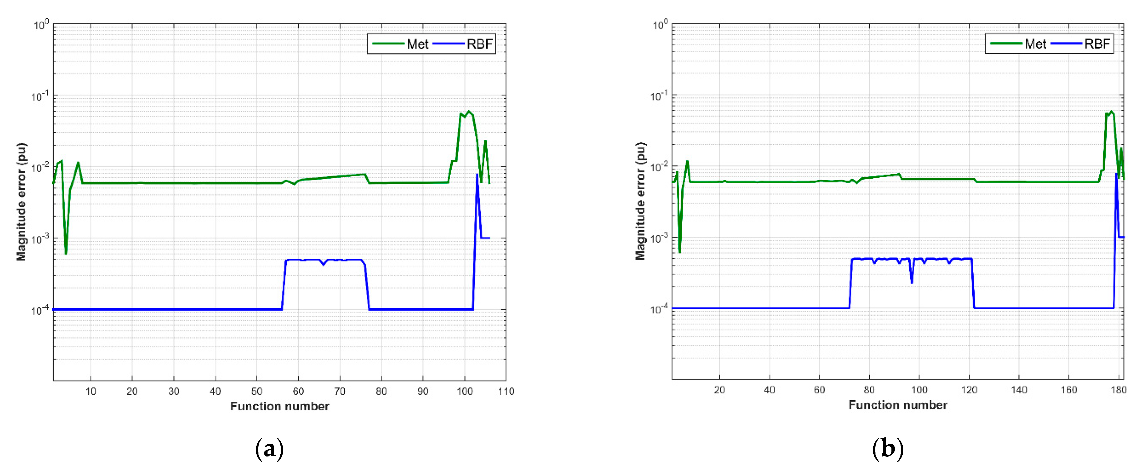
  • The idea of using two algorithms operating simultaneously to estimate the synchrophasor magnitude, phase and frequency that applied identical calculation methods; the main difference between them was that the first one filtered the input signal using the FIR filter, while the second one operated without any filter;
  • The method of the synchrophasor magnitude estimation by means of a suitably trained and applied RBF;
  • The algorithm calculating corrections of the phase shift between the input and output signal;
  • The algorithm calculating corrections of the magnitude estimation;
  • The algorithm of phase estimation using the phase from the previous measurement window and the frequency value from a given window.
In addition, the RBF method applied in the studies was characterized by the speed and accuracy of the results obtained, which is an important issue when researching the dynamic states of the electrodynamic system, especially when overvoltage or other system failures occur.
The RBF method presented in this article can be used in a real power system as an alternative to the algorithms for processing samples in PMU devices described in the literature; e.g., in the calculation of the transmission line parameters using PMU measurements from the two ends of the transmission line [42] (herein the authors presented the scheme processing the samples using algorithms’ FFT in PMU devices), or in the distributed generation system, in which the PMU device is used to monitor the system [43].

Author Contributions

Conceptualization, M.B., A.K. and P.R.; methodology, M.B. and A.K.; software, M.B. and A.K.; validation, M.B., A.K. and P.R.; formal analysis, M.B. and A.K.; investigation, M.B.; resources, M.B.; data curation, M.B.; writing—original draft preparation, M.B., A.K. and P.R.; writing—review and editing, M.B., A.K. and P.R.; visualization, M.B.; supervision, A.K.; project administration, M.B. and A.K. All authors have read and agreed to the published version of the manuscript.

Funding

This research received no external funding.

Conflicts of Interest

The authors declare no conflict of interest.

References

  1. Machowski, J. Wide-area measurement system applied to emergency control of power system Part I Synchronous phasor measurement. Autom. Elektroenerg. 2005, 2, 26–34. [Google Scholar]
  2. IEEE Standard for Synchrophasor Measurements for Power Systems. In IEEE Std C37.118.1-2011 (Revision of IEEE Std C37.118TM-2005); IEEE: Piscataway, NJ, USA, 2011; pp. 1–61. [CrossRef]
  3. IEEE. IEEE Standard for Synchrophasors for Power Systems Measurements for Power Systems–Amendment 1: Modification of Selected Performance Requirements. In IEEE Std C37.118.1a–2014 (Amendment to IEEE Std C37.118.1-2011); IEEE: Piscataway, NJ, USA, 2014; pp. 1–25. [Google Scholar] [CrossRef]
  4. International Electrotechnical Commission. IEC/IEEE Standard 60255-118-1:2018 Part 118-1: Synchrophasor Measurements for Power Systems; IEEE STD23444; International Electrotechnical Commission: Geneva, Switzerland, 2018; pp. 1–78. ISBN 978-1-5044-5361-5. [Google Scholar] [CrossRef]
  5. Phadke, A.G.; Thorp, J.S. Synchronized Phasor Measurements and Their Applications; Springer: New York, NY, USA, 2008; pp. 5–195. [Google Scholar]
  6. Femine, A.D.; Gallo, D.; Landi, C.; Luiso, M. The Design of a Low Cost Phasor Measurement Unit. Energies 2019, 12, 2648. [Google Scholar] [CrossRef] [Green Version]
  7. Li, J.; Wei, W.; Zhang, S.; Li, G.; Gu, C. Conditional Maximum Likelihood of Three-Phase Phasor Estimation for µPMU in active Distribution Networks. Energies 2018, 11, 1320. [Google Scholar] [CrossRef] [Green Version]
  8. Kang, S.-H.; Seo, W.-S.; Nam, S.-R. A Frequency Estimation Method Based on a Revised 3-Level Discrete Fourier Transform with an Estimation Delay Reduction Technique. Energies 2020, 13, 2256. [Google Scholar] [CrossRef]
  9. Kušljević, M.D.; Tomić, J.J.; Poljak, P.D. On Multiple-Resonator-based Implementation of IEC/IEEE Standard P-Class Compliant PMUs. Energies 2021, 14, 198. [Google Scholar] [CrossRef]
  10. Xue, H.; Cheng, Y.; Ruan, M. Enhanced Flat Window-Based Synchrophasor Measurement Algorithm for P Class PMUs. Energies 2019, 12, 4039. [Google Scholar] [CrossRef] [Green Version]
  11. Rebizant, W.; Szafran, J. Power system frequency estimation. IET Gener. Transm. Dis. 1998, 145, 578–582. [Google Scholar] [CrossRef] [Green Version]
  12. Szafran, J.; Wiszniewski, A. Measurement and Decision Algorithms of Digital Protection and Control; WNT: Warszawa, Poland, 2001. (In Polish) [Google Scholar]
  13. Thilakarathne, C.; Meegahapola, L.; Fernando, N. Static Performance Comparison of Prominent Synchrophasor Algorithms. In Proceedings of the 2017 IEEE Innovative Smart Grid Technologies-Asia, Auckland, New Zealand, 4–7 December 2017; pp. 1–6. [Google Scholar] [CrossRef]
  14. Thilakarathne, C.; Meegahapola, L.; Fernando, N. Improved Synchrophasor Models for Power System Dynamic Stability Evaluation Based on IEEE C37.118.1 Reference Architecture. IEEE Trans. Instrum. Meas. 2017, 66, 2937–2947. [Google Scholar] [CrossRef]
  15. Roscoe, A.J.; Abdulhadi, I.F.; Burt, G.M. P–Class Phasor Measurement Unit Algorithms Using Adaptive Filtering to Enhance Accuracy at Off-Nominal Frequencies. In Proceedings of the 2011 IEEE International Conference on Smart Measurements of Future Grids, Bologna, Italy, 14–16 November 2011; pp. 1–8. [Google Scholar] [CrossRef] [Green Version]
  16. Roscoe, A.J.; Abdulhadi, I.F.; Burt, G.M. P and M Class Phasor Measurement Unit Algorithms Using Adaptive Cascaded Filters. IEEE Trans. Power Deliv. 2013, 28, 1447–1459. [Google Scholar] [CrossRef] [Green Version]
  17. Roscoe, A.J. Exploring the Relative Performance of Frequency-Tracking and Fixed-Filter Phasor Measurement Unit Algorithms Under C37.118 Test Procedures, the Effects of Interharmonics, and Initial Attempts at Merging P-Class Response With M-Class Filtering. IEEE Trans. Instrum. Meas. 2013, 62, 2140–2153. [Google Scholar] [CrossRef] [Green Version]
  18. Hsieh, G.; Hung, J.C. Phase-locked loop techniques. A survey. IEEE Trans. Ind. Electron. 1996, 43, 609–615. [Google Scholar] [CrossRef]
  19. Dash, P.K.; Jena, R.K.; Panda, G.; Routray, A. An extended complex Kalman filter for frequency measurement of distorted signals. IEEE Trans. Instrum. Meas. 2000, 49, 746–753. [Google Scholar] [CrossRef] [Green Version]
  20. Girgis, A. A new Kalman filtering based digital distance relay. IEEE Power Eng. Rev. 1982, PAS-101, 3471–3480. [Google Scholar]
  21. De Apráiz, M.; Diego, R.I.; Barros, J. An Extended Kalman Filter Approach for Accurate Instantaneous Dynamic Phasor Estimation. Energies 2018, 11, 2918. [Google Scholar] [CrossRef] [Green Version]
  22. Kamwa, I.; Samantaray, S.R.; Joos, G. Compliance Analysis of PMU Algorithms and Devices for Wide-Area Stabilizing Control of Large Power Systems. IEEE Trans. Power Syst. 2013, 28, 1766–1778. [Google Scholar] [CrossRef]
  23. Kamwa, I.; Samantaray, S.R.; Joos, G. Wide Frequency Range Adaptive Phasor and Frequency PMU Algorithms. IEEE Trans. Smart Grid 2014, 5, 569–579. [Google Scholar] [CrossRef]
  24. Ren, J.; Kezunovic, M. Real-Time Power System Frequency and Phasors Estimation Using Recursive Wavelet Transform. IEEE Trans. Power Deliv. 2011, 26, 1392–1402. [Google Scholar] [CrossRef]
  25. De la Serna, J.A. Synchrophasor Estimation Using Prony’s Method. IEEE Trans. Instrum. Meas. 2013, 62, 2119–2128. [Google Scholar] [CrossRef]
  26. Kasztenny, B.; Premerlanit, W.; Adamiak, M. Synchrophasor Algorithm Allowing Seamless Integration with Today’s Relays. In Proceedings of the 2008 IET 9th International Conference on Developments in Power System Protection, Glasgow, UK, 17–20 March 2008; pp. 724–729. [Google Scholar] [CrossRef]
  27. Premerlani, W.; Kasztenny, B.; Adamiak, M. Development and Implementation of a Synchrophasor Estimator Capable of Measurements under Dynamic Conditions. IEEE Trans. Power Deliv. 2008, 23, 109–123. [Google Scholar] [CrossRef]
  28. Sykes, J.; Koellner, K.; Premerlani, W.; Kasztenny, B.; Adamiak, M. Synchrophasors: A Primer and Practical Applications. In Proceedings of the 2007 Power Systems Conference: Advanced Metering, Protection, Control, Communication and Distributed Resources, Clemson, SC, USA, 13–16 March 2007; pp. 1–26. [Google Scholar] [CrossRef]
  29. Tanvir, A.A.; Merabet, A. Artificial Neural Network and Kalman Filter for Estimation and Control in Standalone Induction Generator Wind Energy DC Microgrid. Energies 2020, 13, 1743. [Google Scholar] [CrossRef] [Green Version]
  30. Cichocki, A.; Łobos, T. Adaptive analogue network for real-time estimation of basic waveforms of voltages and currents. IEEE Proc. C 1992, 139, 343–350. [Google Scholar] [CrossRef]
  31. Osowski, S. Neural network for estimation of harmonic components in a power system. IEEE Proc. C 1992, 139, 129–135. [Google Scholar] [CrossRef]
  32. Chen, C.-I.; Chen, Y.-C.; Chin, Y.-C.; Wang, H.-L. Design of Neural Network-Based Phasor Measurement Unit for Monitoring of Power System. In Proceedings of the 2014 IEEE International Conference on Granular Computing, Noboribetsu, Hokkaido, Japan, 22–24 October 2014; pp. 45–48. [Google Scholar] [CrossRef]
  33. Innah, H.; Hiyama, T. Neural Network Method Based on PMU data for Voltage Stability Assessment and Visualization. In Proceedings of the TENCON 2011–2011 IEEE Region 10 Conference, Bali, Indonesia, 21–24 November 2011; pp. 822–827. [Google Scholar] [CrossRef]
  34. Ivanov, O.; Gavrilaş, M. State Estimation with Neural Networks and PMU Voltage Measurements. In Proceedings of the 2014 International Conference and Exposition on Electrical and Power Engineering, Iasi, Romania, 16–18 October 2014; pp. 983–988. [Google Scholar] [CrossRef]
  35. Kamwa, I.; Grondin, R.; Sood, V.K.; Gagnon, C.; Nguyen, V.T.; Mereb, J. Recurrent Neural Networks for Phasor Detection and Adaptive Identification in Power System Control and Protection. IEEE Trans. Instrum. Meas. 1996, 45, 657–664. [Google Scholar] [CrossRef]
  36. Binek, M.; Kanicki, A.; Korbel, P. Signal Parameters Identification Methods Used in Wide-Area Measurement Systems. In Proceedings of the 2016 Electrical Power Networks Conference–EPNet, Szklarska Poreba, Poland, 19–21 September 2016; pp. 1–5. [Google Scholar] [CrossRef]
  37. Mohagheghi, S.; Venayagamoorthy, G.; Harley, R. Optimal wide area controller and state predictor for a power system. IEEE Trans. Power Syst. 2007, 22, 693–705. [Google Scholar] [CrossRef]
  38. Gong, J.; Yang, W. Driver Pre-accident Behaviour Pattern Recognition Based on Dynamic Radial Basis Function Neural Network. In Proceedings of the 2011 International Conference on Transportation, Mechanical and Electrical Engineering, Changchun, China, 16–18 December 2011; pp. 328–331. [Google Scholar] [CrossRef]
  39. Castello, P.; Liu, J.; Muscas, C.; Pegoraro, P.A.; Ponci, F.; Monti, A. A Fast and Accurate PMU Algorithm for P+M Class Measurement of Synchrophasor and Frequency. IEEE Trans. Instrum. Meas. 2014, 63, 2837–2845. [Google Scholar] [CrossRef]
  40. Castello, P.; Muscas, C.; Pegoraro, P.A.; Sulis, S.; Toscani, S. Experimental Characterization of Dynamic Methods for Synchrophasor Measurements. In Proceedings of the 2014th IEEE International Workshop on Applied Measurements for Power Systems Proceedings, Aachen, Germany, 24–26 September 2014; pp. 1–6. [Google Scholar] [CrossRef]
  41. Toscani, S.; Muscas, C. A Space Vector Based Approach for Synchrophasor Measurement. In Proceedings of the 2014 IEEE International Instrumentation and Measurement Technology Conference, Montevideo, Uruguay, 12–14 May 2014; pp. 1–5. [Google Scholar] [CrossRef] [Green Version]
  42. Hareesh, S.V.; Raja, P.; Selvan, M.P. An Effective Implementation of Phasor Measurement Unit (PMU) by using Non-Recursive DFT Algorithm. In Proceedings of the 2015 International Conference on Condition Assessment Techniques in Electrical Systems (CATCON), Bangalore, India, 10–12 December 2015; pp. 195–199. [Google Scholar] [CrossRef]
  43. De la O Serna, J.A.; Paternina, M.R.A.; Zamora-Mendez, A. Assessing Synchrophasor Estimates of an Event Captured by a Phasor Measurement Unit. IEEE Trans. Power Deliv. (Early Access) 2020, 1–9. [Google Scholar] [CrossRef]
Figure 1. The flowchart of the algorithm for converting instantaneous voltage or current values into the synchrophasor parameters.
Energies 14 02570 g001
Figure 2. The correction of a phase shift introduced by the FIR filter as a function of the input signal frequency.
Energies 14 02570 g002
Figure 3. The magnitude estimation correction as a function of the input signal frequency.
Energies 14 02570 g003
Figure 4. The TVE, FE and RFE graphs for subsequent functions: (a) data for the P class of the PMU device; (b) data for the M class of the PMU device.
Energies 14 02570 g004
Figure 5. The RT-TVE, RT-FE and RT-RFE graphs for subsequent functions: (a) data for the P class of the PMU device; (b) data for the M class of the PMU device.
Energies 14 02570 g005
Figure 6. The DT and OV graphs for subsequent functions: (a) data for the P class of the PMU device; (b) data for the M class of the PMU device.
Energies 14 02570 g006
Figure 7. The magnitude error graphs for subsequent functions: (a) data for the P class of the PMU device; (b) data for the M class of the PMU device.
Energies 14 02570 g007
Table 1. Permissible measurement error values of synchrophasor parameters.
P ClassM Class
Function NumberTVEFERFEFunction NumberTVEFERFE
%HzHz/s%HzHz/s
110.0050.4110.0050.1
2, 310.0050.42, 310.0050.1
4 ÷ 710.0050.44 ÷ 710.0050.1
8 ÷ 5610.0050.48 ÷ 5610.025-
----57 ÷ 721.30.01-
57 ÷ 7630.062.373 ÷ 12230.314
77 ÷ 9630.062.3123 ÷ 17230.314
97, 9810.010.4173, 17410.010.2
Step Functions—Response Times
Function NumberRT-TVERT-FERT-RFEFunction NumberRT-TVERT-FERT-RFE
SSssss
99÷1020.040.090.12175 ÷ 1780.140.280.28
103÷1060.040.090.12179 ÷ 1820.140.280.28
Step Functions—Delay Time and Overshoot/Undershoot Value
Function NumberDTOV-Function NumberDTOV-
S%-s%-
99 ÷ 1020.0055-175 ÷ 1780.00510-
103 ÷ 1060.0055-179 ÷ 1820.00510-
Publisher’s Note: MDPI stays neutral with regard to jurisdictional claims in published maps and institutional affiliations.

