Article

A Substitutive Coefficients Network for the Modelling of Thermal Systems: A Mono-Zone Building Case Study

by
Lahoucine Ouhsaine
1,2,
Mohammed El Ganaoui
1,
Abdelaziz Mimet
2 and
Jean-Michel Nunzi
1,3,4,*
1
Department of Thermal and Energy Engineering, LERMAB, IUT Henri Poincaré, University of Lorraine, 54400 Longwy, France
2
Energetic Laboratory, Faculty of Sciences, Abdelmalek Essaâdi University, Tétouan 93030, Morocco
3
Department of Chemistry, Queen’s University, Kingston, ON K7L-3N6, Canada
4
Department of Physics, Engineering Physics and Astronomy, Queen’s University, Kingston, ON K7L-3N6, Canada
*
Author to whom correspondence should be addressed.
Energies 2021, 14(9), 2551; https://doi.org/10.3390/en14092551
Submission received: 14 March 2021 / Revised: 23 April 2021 / Accepted: 25 April 2021 / Published: 29 April 2021
(This article belongs to the Section J: Thermal Management)

Abstract

:
A modelling approach based on the Substitutive Coefficients Network (SCN) is developed to predict the thermal behavior of a system in the dynamic state-space, without requiring knowledge of the thermal mass. The method can apply either to large- (building, combined solar systems, geothermal energy, and thermodynamic installations) or to small-scale systems (heat exchangers, electronic devices cooling systems, and Li-ion batteries). This current method is based on a dimensionless formulation of the simplified dynamic thermal balance model, using relaxation time as a key parameter to establish the model. The introduction of relaxation time reduces the parameters set as guidance coefficients. The parameters are finally expressed by a combination of global heat transfer coefficients related to each layer and/or sub-layer of the system. Advantages of the method are reliability, “non-destructibility”, i.e., it allows a reliable prediction of the thermal behavior which experimentally is inaccessible, and reducibility of the parameters size estimate. Additionally, the method is inexpensive in terms of computation memory. It is also easy to implement in practical numerical schemes. In this paper, the method leads to a simplified mathematical model that predicts the thermal behavior of a mono-zone eco-cottage building installed at Lorraine University (in Longwy, France) as a case study. Thermal performance of the building is estimated under the hourly weather conditions onsite, as obtained from the Meteonorm software. The thermal dynamics within hourly Typical Meteorological Year 2 (TMY2) Meteonorm data disturbances and the internal heating input state in the winter period were simulated with a simplified numerical discretization method. Results provide a general dynamic state of the different sub-components of the system, with limited design of the model parameters.

Graphical Abstract

1. Introduction

The evolution of thermal energy systems is a subject of major importance today. It is also considered a very complex problem in terms of geometry and sub-system coupling methods. Despite complexity, the aim is to enhance the efficiency and thermal performances of thermal processes. Several methods were used to model and to better simulate the thermal behavior. The technique of simplified or “reduced-order models” gets a special attention as it performs better for temperature estimation. 
In full-scale systems, research and methods were dedicated at simplifying thermodynamic models and substituting  computational fluid dynamics (CFD) numerical codes. In the particular case of buildings, Zhu et al. [1] presented a simplified dynamic model for pipe-embedded building envelopes, also considering phase change materials (PCM) to enhance thermal benefits. The authors use the frequency domain finite difference (FDFD) method to separate capacity and resistance impedances using complex and eal numbers. Despite the performance of the model to predict the thermal dynamic behavior for some geometrical points, the simplified model still does not predict some configurations and it is hard to generalize it to complex geometries as the authors suggested. Soria-Verdugo et al. [2] proposed a simplified lumped capacitance model integrated into a theoretical distributed activation energy model to estimate multi-physics dependent behaviors in the pyrolysis biomass processes. Based on thermal balances, Belmonte et al. [3] suggested a simplified model for thermal energy storage systems including phase change materials, which can be used for any type of thermal energy storage system. Gao et al. [4] developed a simplified thermal model for the indoor environment of rooms with Chinese kang bed-stoves. They propose a matrix formulation of the main state temperatures dependent on three types of parameters, like thermal, geometrical, and data. Their model however is still limited to the air temperature with lower accuracy as they claimed. Furthermore, the number of parameters is still very large, and it is hard to control the dynamic simulation of the model with accuracy. Al Assad et al. [5] conducted experiments and propose a simplified thermal coupled heat and mass transfer model for the internal air quality in a conditioned room. The objective of their work is to save energy on the air conditioning system. Fine et al. [6] suggested a simplified steady-state model for the long-term thermal effect of solar assisted ground source heat pump systems. Gao et al. [7] presented a classical lumped resistance-capacitance (RC) model for a paraffin based PCM layer. They optimize the RC decomposition in the sample by fitting the experimental data with a genetic algorithm. Kharbouch et al. [8] investigated the thermal performance using a dynamic simplified lumped capacitance RC model for building envelopes integrated PCMs. They estimate the time-lag and decrement factor as a characterization results for their model.
At smaller scales, in modern power electronics, the thermal behavior is usually predicted by dynamic models. CFD techniques are very useful to estimate the temperature dynamics in microchips [9,10]. Simplified models are also applied to estimate at low memory computation the thermal dynamics in electronic devices. Bouguezzi et al. [11] simplified the analytical thermal model of a multi-chip power module. The model mainly describes analytically the thermal impedance with respect to the geometry.
At larger scales, case studies using simplified and lumped capacitances based on the first law of thermodynamic recently got attention in buildings and renewable energy systems. Two major reasons justify this interest: First, the need for simulation frameworks that can predict fast and accurately according to meteorological data variations the thermal behavior of each sub-component of the system, and that can substitute to the heavy CFD codes in the dynamic regime. Second, the evolution of genetic algorithms and neural network methods to estimate accurately the thermo-physical parameters and output functions of the system. Nevertheless, the growing complexity of thermal energy systems complicates even those simplified models by gathering the behaviors of the sub-components of the system.
To summarize with the three above cited scales (full, small, and large), thermal methods may depend on the scale and on the thermal processes. However, literature shows the importance of building a unified simple model to better represent the thermal system dynamics [12]. The state-space method was a subject of development for both linear and non-linear systems [13,14,15,16,17,18]. Furthermore, in thermal dynamics, the method gets interesting for its flexibility and ease-of-implementation in control and optimization models. Ouhsaine et al. [16] developed a state-space formulation for complex building integrated solar systems with phase change materials and performed an analysis within climate conditions variations. Chen et al. [19] used a data driven state-space Wiener model to characterize the dynamic relation between climatic condition variations and the resultant thermal sensation of the occupant. Using a state-space model, Yao et al. [20] developed a three zone thermal dynamic response in existing rooms. Their works emphasize the ability of the state-space representation to predict in real-time the thermal response in the rooms.
The present research aims at simplifying the complexity of coupled system models by using a dimensionless state-space formulation. Both the thermal resistance and the lumped capacitance are represented by one substitutive impedance which can be obtained by the introduction of a relaxation time into the heat transfer differential equation. The parameters obtained from the heat thermal balance are identified and classified into proper and external parameters. Furthermore, the goal of this paper is also to show that the novel SCN offers a practical approach to reduce the estimation of the parameter set in the thermal model, especially the heat capacity, and then to surrogate it with a relaxation time which can be measured in real cases. In this work, we present this novel approach, highlighting the importance of the relaxation time to adjust the model.
This paper is organized as follows: the defined methodology for constructing the substitutive coefficient network (SCN) model is presented, based on existing analytical approaches. The main difference with existing dynamic lumped capacitance RC methods is highlighted. The relevant properties that define the operation limits of the model are also presented. The full-scale case study of a mono-zone building model is presented to validate the method. Prospective applications are foreseen with studying the interaction of heat transfer and fluid flow in the mono-zone building and their influence on the indoor air quality and occupancy comfort [21].

2. Methodology

We emphasize the methodology used in this paper in order to compare the lumped capacitance model with the developed SCN method. From the heat transfer equation, a lumped capacitance model is determined, then by using the dimensionless formulation and relaxation time integration, a novel formulation is obtained from the multi-components of the system. It is easily to represent the thermal state of all the component of the system into one single state-space equation which represents an advantage in the simplification of thermal systems modelling.

2.1. Lumped Capacitance Models

Based on the first law of thermodynamic, the lumped capacitance method is a simplified solution of the Laplace law and specifically of the heat equation bellow:
ρ c T t = k ² T x ² + S
where   ρ   ( m 3 / kg ) , c   ( J / kg . K ) , k   ( W / m . K ) , and S   ( W / m 3 ) are respectively, the density, the heat capacity, the thermal conductivity, and the volumetric power source density.
In order to explore the lumped capacitance model, the example of a uniform 1D wall is presented in Figure 1.
The heat equation for the wall can be integrated from 0 to L into Equation (2)
ρ c T ¯ t = k ( T ¯ x L , t T ¯ x 0 , t )
By definition, the right-hand term in the equation is the difference of the heat fluxes between 0 to L expressed by the Fourier law. Therefore:
ρ c T ¯ t = φ 0 ( t ) φ L ( t )
φ 0 ( t ) is the incoming heat flux, and φ L ( t ) is the outgoing heat flux as described by heat balance in Equation (3). Integration of the heat fluxes can be expressed linearly for   q 0 ( t ) = U 0 ( T 0 T ¯ ) , and U L ( T ¯ T L ) . It can be noted that some approaches detailed and extended the heat fluxes balances to the medium surrounding the wall with inclusion of heat transfer coefficients by convection h 0 and h L , to represent the model with boundary conditions. The relationship highlighting this is defined by the reference temperature as: T r e f = ( h 0 T 0 + q 0 + h L T L q L ) ( h 0 + h L ) . Therefore, T ¯ ( t ) can be expressed by resolving Equation (3). Introducing the expression of T r e f and initial condition   T i , we get:
T ¯ ( t ) = T r e f + ( T i T r e f ) e t t c
where t c = k L a ( h 0 + h L ) is the relaxation time (the maximum time needed to reach the stationary regime). Some analytical solutions of the full 1D heat equation with boundary conditions were proposed in the literature [22]. In this lumped capacitance model, the approach is very useful for full scale buildings (walls and indoor ambient). However, as long as the components are added to the “wall system”, and its size increases, the parameters are multiplied according to the number of state temperatures and the behavior itself. Despite efforts on reducing-order thermodynamic models, modeling in this case remains a delicate task. It is necessary for that purpose to design a technique that helps organizing the structure of the model, it is also more judicious to group the parameters in one unified frame, which mainly synchronizes the parameters and the variables with the behavior itself. Therefore, our novel technique is proposed as the basis of this reasoning.

2.2. Alternative SCN Model

The methodology in our approach consists into transforming the physical dimensional space into the mathematical dimensionless one by using a dimensionless formulation applied to a discrete form of the Equation (3).
Let us express the relaxation time for the wall case by:
t c = k L a ( h 0 + h L )
where a = k C is the thermal diffusivity, C = ρ c is the thermal mass, L is the relaxation length, and   h e x t = h 0 + h L are external heat transfer coefficients by convection. Upon substituting the diffusivity term in the Equation (5), the relaxation time becomes:
t c = C L   h e x t
The t c obtained in Equation (6) can be generalized to the local formula by:
t c = C   U e x t
where   U e x t is the external global heat transfer coefficient of a considered local thermal body. Therefore, applying the dimensionless technics to the simplified form of the (1 + 1)D heat transfer defined by Equation (8), the simplified dimensionless heat transfer equation with source terms is written as:
C T t = U e i n ( T 0 T ) U p ( T T L ) + S    
θ τ = q ( θ 0 θ ) p ( θ θ L ) + 𝓈 S ¯    
where q = U e i n i N U e i n + i N U e o u t and p = U p i N U e i n + i N U e o u t refer respectively to the named external inputs and proper parameters.   S ¯ = S S m a x ,   θ = T T r e f T m a x T r e f , and τ = t t c . The local formula for a linear model can be expressed by Equation (10):
θ τ = r Δ θ + 𝓈 S ¯
Equation (10) can be resolved if and only if the boundary and initial conditions are specified., S ¯ is the local term source, and r θ is the diffusive term. The simplified model can be represented analytically as shown by Equation (9), but also algebraically for combined and coupled sub-systems. Advantage of the algebraic representation is its flexibility to design a controller system, as well as a practical approach to optimize the design of the system or even its thermal behavior regardless its complexity. The linear algebraic formulation for infinite dimensions is represented by Equation (11).
θ ˙ ( τ ) = A ( r ) θ ( τ ) + B u 1 P ¯ ( τ ) + B w 1 ( r ) θ e ( τ ) + B w 2 ( s ¯ ) φ ¯ s ( τ )
where θ ˙ = θ τ is the temperature differential temporal behavior. In order to determine optimally the size of the matrices, we propose the criterion defined by Equation (12), which is based on the generalized Biot number.
ο j = i = 1 N p i j < ε
where   ε represents the thermal thin layer coefficient defined by Biot, physically the layer is considered as thermally thin if and only if ε 0.1 . The r parameters of the matrices A can be classified into two categories: the proper parameters p = U p   U e which are located in the upper triangular part of the matrix, and the q = U e i n   U e parameters who are classified as external input ones, which are located at the lower triangular part of the matrix   A .
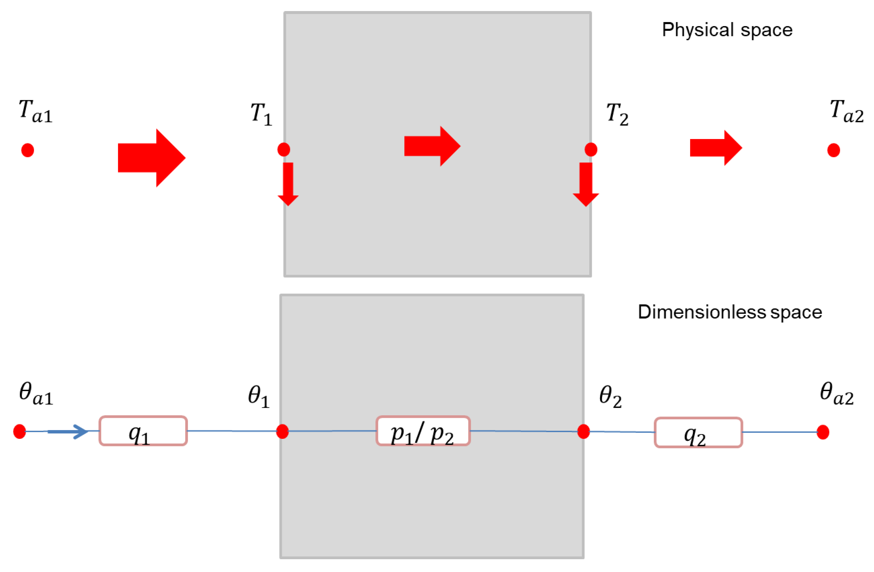
The algebraic model can substitute the RC approach by one dimensionless r impedance. Reading of the r ( q , p ) network can be qualified as a substitutive impedance network as represented in Figure 2, because thermal balance at the nodes is dynamically following the substitution process of r ( q , p ) impedance variation and heat fluxes.
The methodology described above leads to one state-space equation in a dimensionless formulation as described by Equation (11). In order to emphasize the method, it is worth applying it in a practical case. The following shows a practical example of application of the SCN method with a numerical simulation.

3. Mono-Zone Building Case Study

In the present work, an isolated mono-zone building is studied with the above developed model. The building is an eco-cottage (Figure 3) situated at Longwy city (Lorraine University, North East of France, 300 m above the sea level, 49.52° N and 5.769° E), constructed by Laboratory of Studies and Research on Wood Materials using high thermo-physical performance materials [23,24].
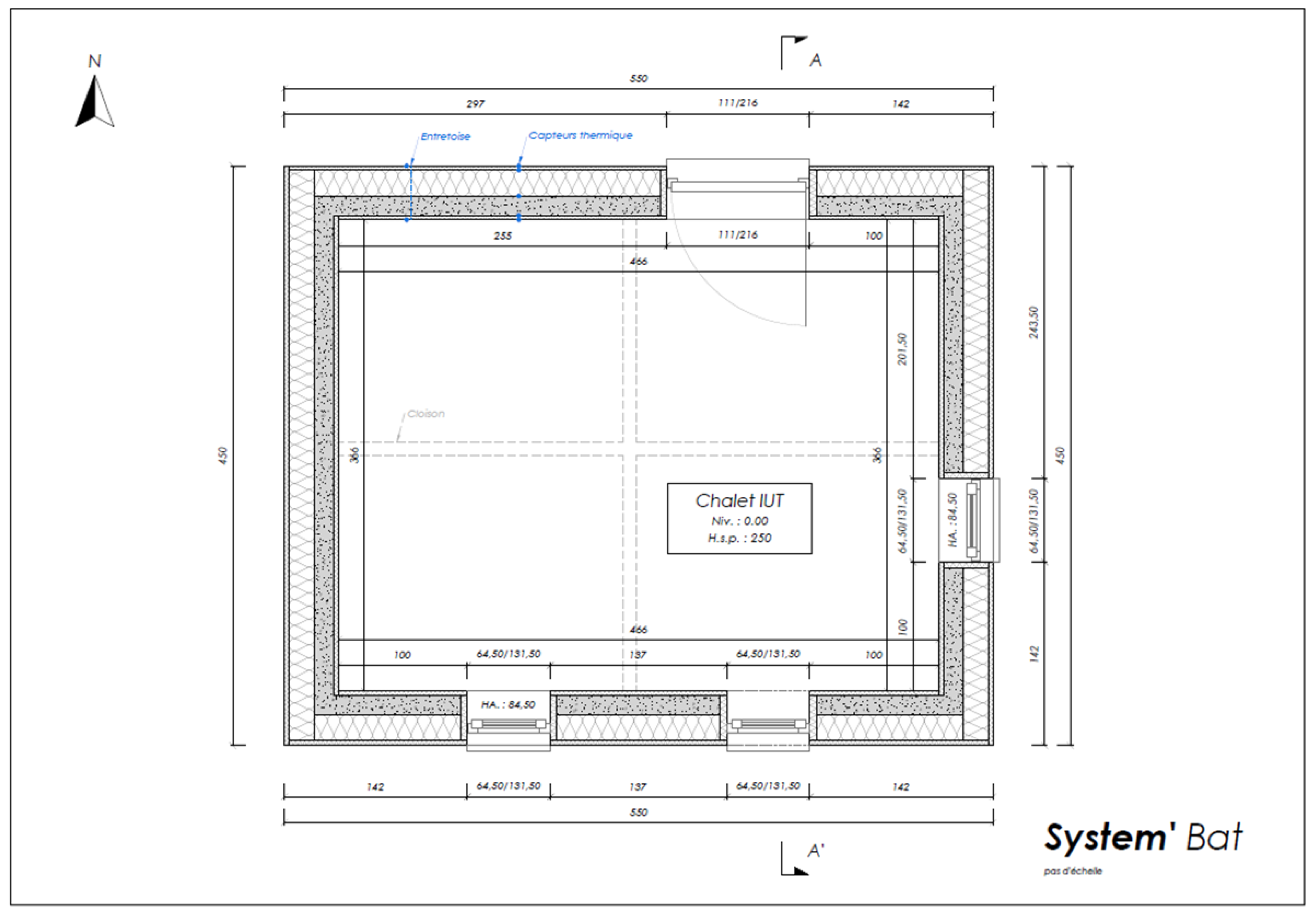
The eco-cottage area is 25 m². It is composed of a single room with a 2.4 m² door on the north side (double glazed) and three 0.84 m² windows; one oriented east and two other south. The roof is slanted by 5° to the south for the evacuation of waters rain (Figure 3).
The algebraic thermal model applied is defined in Equation (13), where   A , B u , B w 1 , and B w 2 are defined in the Nomenclature. The r ( q , p ) parameters are defined for each layer in Table 1. In order to simplify the approach, some physical assumptions are made as:
  • Thermal bridges are neglected,
  • Thermal impedance between the nodes on the same level is neglected,
  • Indoor air temperature is assumed uniform,
  • Indoor air velocity is assumed very low,
  • Contact impedance is neglected,
  • Reference temperature is taken as the external ambient one.
Based on these assumptions, the input term B u ( v ¯ ) θ ( ξ , τ ) is neglected and Equation (13) becomes:
θ ˙ ( τ ) = A ( r ) θ ( τ ) + B u 1 P ¯ ( τ ) + B w 2 ( s ) φ ¯ s ( τ )
The thermal SCN network for the eco-cottage is shown in Figure 4, where the heat flux is permuted between r(q,p) impedances from the heat source represented by inputs, to the “large heat sink” represented by external disturbances. The inertial term that represents the thermal mass is considered useless in the SCN scheme; even though the model is developed in the transient regime.
The eco-cottage described in this part by the thermal SCN scheme can be resolved numerically. In Figure 4, the external disturbances are the discrete climatic conditions applied by the term B w 1 ( r ) θ e ( τ ) + B w 2 ( s ¯ ) φ ¯ s ( τ ) . The known input internal power is introduced by discrete values. Thereafter, a numerical model is used to apply the mathematical model.

4. Numerical Simulation

4.1. Numerical Scheme

In order to simulate the thermal behavior represented by Equation (13), a numerical model based on a simple explicit discretization is proposed by [16] and described by:
θ ( j + 1 ) = ( 𝕝 A ) 1 [ θ ( j ) + ( B u 1 P ¯ ( j ) + B w 2 φ ¯ s ( j ) ) ]
where   j is the time increment, 𝕝 is the identity matrix, and ( 𝕝 A ) 1 is the inverse matrix.

4.2. Model Adjustment

The model adjustment is about determining the relaxation time. In a dimensionless space, it can be seen that the materials have one singular thermal behavior.
The simulation example to adjust the SCN model considers the validation with simple lumped capacitance RC model for a single wall with two interactive ambiances. The thermal balance nodes are presented by Figure 4 and
( T ˙ 1 T ˙ 2 ) = [ ( h 0 ρ c p + k ρ c p L ) k ρ c p L k ρ c p L ( k ρ c p L + h L ρ c p ) ] ( T 1 T 2 ) + [ h 0 ρ c p 0 0 h L ρ c p ] ( T a 1 T a 2 )
The dimensionless formulation that provides the SCN model:
( θ ˙ 1 θ ˙ 2 ) = [ ( p 1 + q 1 ) p 1 p 2 ( p 2 + q 2 ) ] ( θ 1 θ 2 ) + [ q 1 0 0 q 2 ] ( θ a 1 θ a 2 )
Equations (14) and (15) have the same form, but the first one is represented in the physical space, while the second one is represented in the mathematical space. The numerical model can be presented using Equation (13) and by:
{ T ( j + 1 ) = ( 𝕝 Δ t A ) 1 [ T ( j ) + Δ t B w 1 T a ( j ) ] θ ( j + 1 ) = ( 𝕝 A ) 1 [ θ ( j ) + B w 1 θ a ( j ) ]
We notice that time t is related to the M numerical discretization points of the SCN model by:
t = M t c
The simulation is conducted for both lumped capacitance and SCN models, the goal of this part is to determine numerically the right relaxation time, and for this reason an algorithm was developed to check the right parameter. Figure 5 represents a simplified thermal behavior in the physical space as represented by nodes and heat fluxes in red color, while in the dimensionless space, the heat fluxes are represented by one single dimensionless flux and cross the qi and pi impedances.
Figure 6 represents the four simulation cases for different relaxation times. The algorithm is running out the file until the SCN temperatures states fitted with the lumped capacitance model. It is also very useful to use this algorithm with experimental results and to implement it in real cases for optimization and control endeavors. The algorithm is based on a simple loop that changes at every sequence t c until T S C N ( t ) = T L C ( t ) .
The model adjustment is a crucial step to validate numerically or experimentally the model in real-time utilization. However, different methods already exist in the literature relevant to the building field, which can be a better alternative to validate the SCN method. In the ANSI/ASHRAE standards [25,26], the BESTEST code can provide analysis and diagnosis for building energy simulation software, software-to-software, and software-to-quasi-analytical solution comparison. This work can be further extended to a validation case such as the ANSI/ASHRAE 140 [25].

5. Results and Discussion

The dynamic simulation of four typical winter days was carried out in this case study by using the Meteo-norm data as external disturbances such as the global heat radiation density, the wind speed, and the ambient temperature. The simulation code was developed on Matlab script and can be run for at least 1 year based on TMY Meteo-norm data for the first days of January 2016. The case study is limited to simulate, especially some cloudy days. Further, the simulation conditions were imposed by the input which represents the heat power supply density. In this simulation scenario we choose 1700 W continuously.
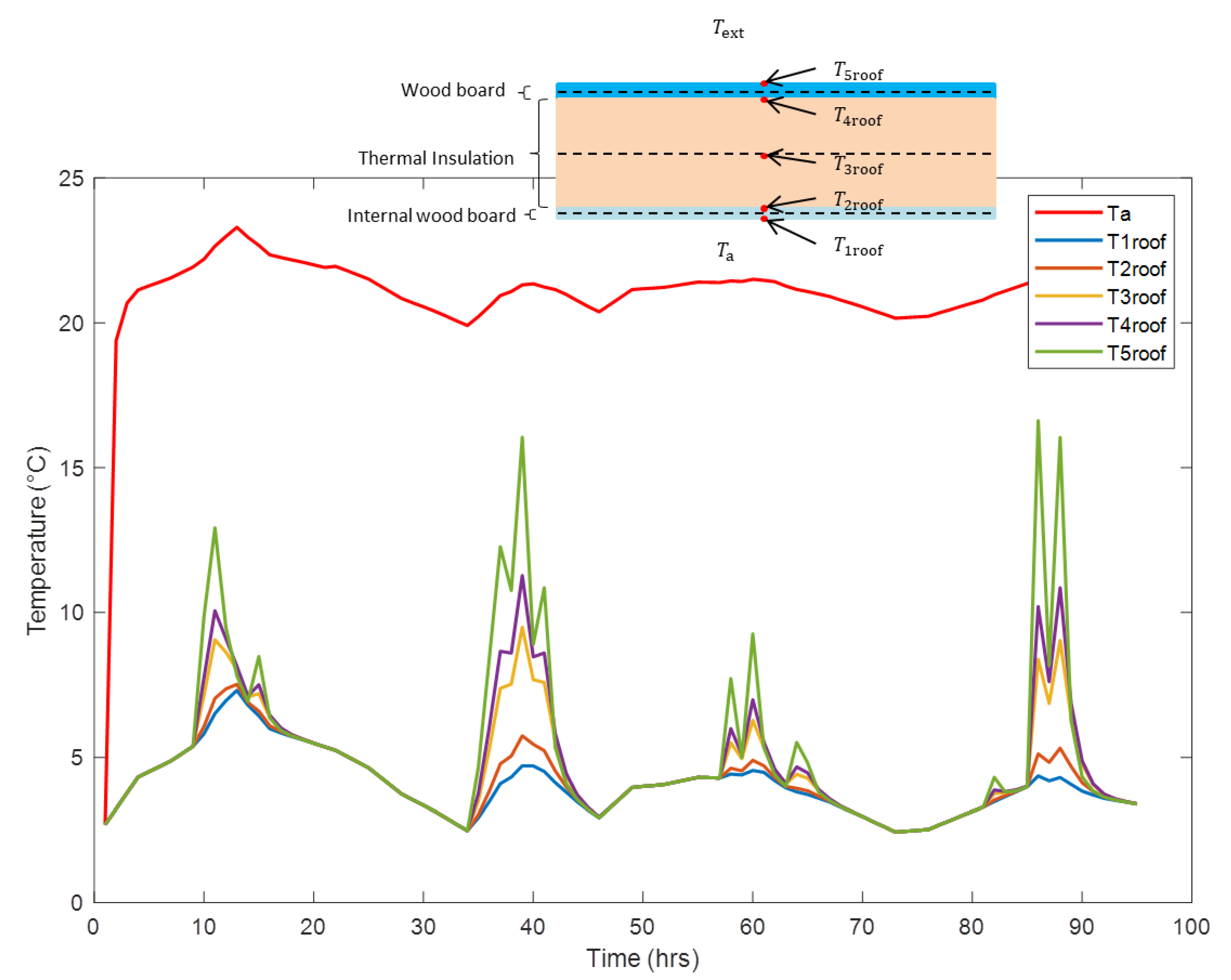
Figure 7 represents the thermal response for the ambient temperature with respect to time as well as the temperature dynamics of the different layers of the roof. It can be seen that the air temperature responds proportionally to the power supply, but it is practically influenced by the external disturbance conditions. While the roof layers temperature dynamics is more influenced by the external temperature and the solar radiation in the daily periods than the internal air temperature that fits its profile during nights, due to the chosen heat convection coefficients, the global parameters design was not subject to optimization in this study.
Figure 8 represents the hourly global solar radiation, the internal air temperature dynamics, the external ambient temperature, and the floor temperature dynamics. The reference temperature is supposed the same as the ambient temperature, the concrete floor layer thicknesses is assumed of 30 cm and subdivided into two sub-layers of 15 cm with thermal conductivity of 0.137 W/m K as well as the insulation part, which is composed of two layers, the first one is considered thermally insulated for 0.142 W/m K and of 10 cm thicknesses while the second, is the floor layer is for 0.318 W/m K and of 3 cm thicknesses. It was seen with these conductance thermal characteristics that the temperature dynamics is in good agreement with the reference temperature, while the ambient internal air temperature still fits with the heat power supply knowing that the heat transfer coefficient is considered for the standard value of 10 W/m²·K.
Figure 9 represents the solar radiation and the internal ambient temperature, the thermal simulation of the door temperature dynamics for both its internal and external sides. As shown in the figure, the temperature differences can be observed clearly between the indoor and the outdoor sides, as well as the daytime temperature evolution which is clearly influenced by the global solar radiation.
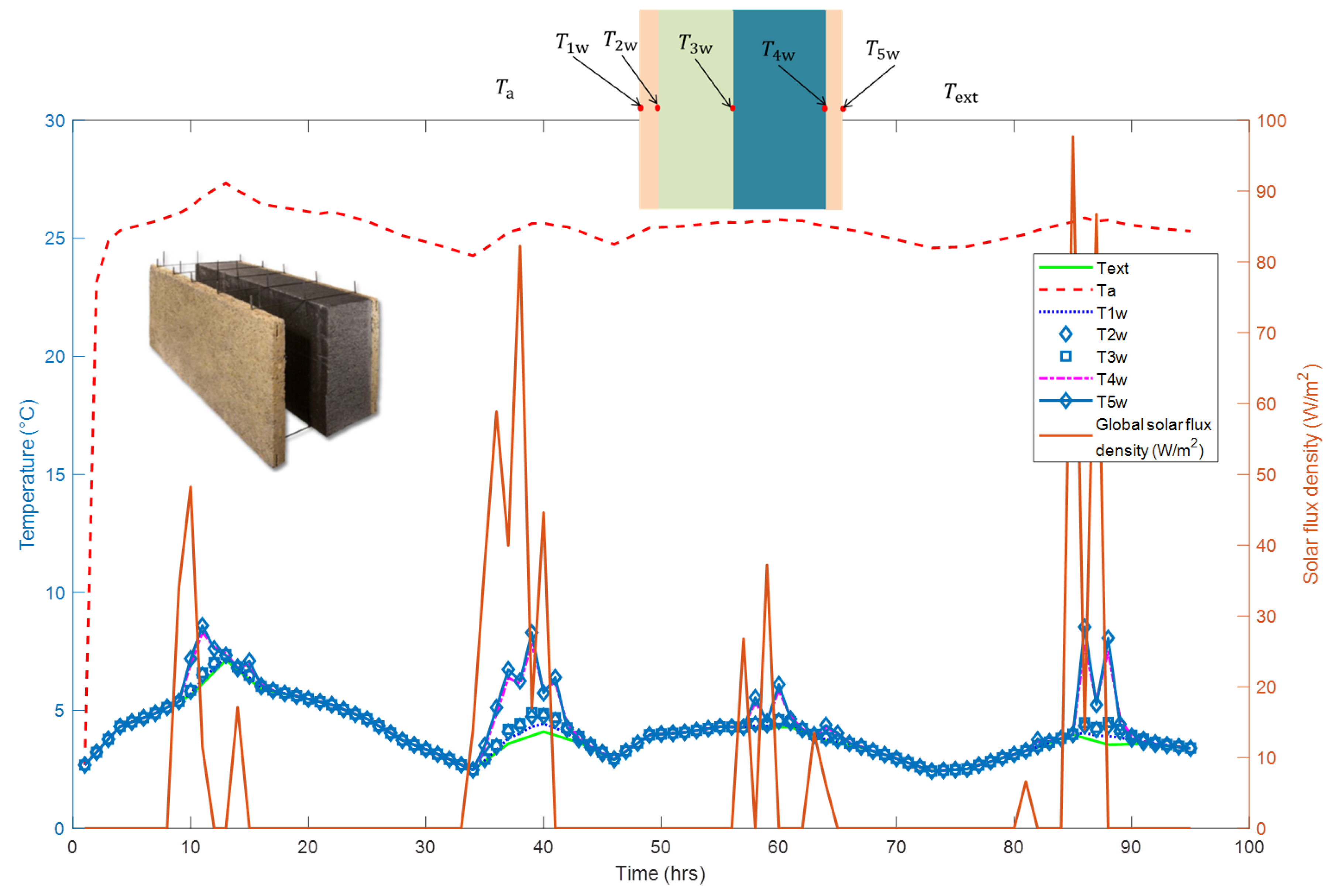
Figure 10 represents further layers of the wall temperature dynamics. As seen in the figure, the external temperature layer is more influenced by the solar radiation than the other sub-layers. That is because the wall is well insulated with 20 cm of polystyrene and 10 cm of concrete.
We clearly observe from the above figures that the behavior of the thermal simulation fits proportionally the external disturbances and the input response from the model. The temperature difference between the indoor air and the other building layers is explained by the heat transfer coefficient which is 10 W/m²·K. The model can also support real experimental data inputs to predict the thermal behavior of the building.

6. Conclusions

This paper introduces an alternative simplified SCN approach to model and simulate the thermal dynamics of an existing mono-zone building. The obtained dynamic results fit equivalently the thermal behavior for classified inputs and external conditions, without requiring the introduction of an inertial term in the model. The developed approach can be expressed into one algebraic equation to model complex thermal systems such as the different components and sub-components of a building. The obtained substitutive coefficients network results provide the general dynamic states of the different sub-components, without limitations on the design of the model parameters. This work also provides an extended version to the complex situation of building simulations involving an active envelop coupled to an adequate energy mix oriented towards passive housing developments. The method permits the integration of an active interaction between the envelop, human occupancy and indoor air quality. Such complex and coupled situation requires more than a simple mathematical verification. Thermal comfort calculations will be conducted in accordance with the ANSI/ASHRAE Standard, to account for the adaptive comfort model which is supposed to vary during the year and to exhibit some singular behavior in particular climates.

Author Contributions

Conceptualization, L.O. methodology, L.O., M.E.G., and J.-M.N.; validation, supervision, A.M. and M.E.G.; investigation, formal analysis, original draft preparation, writing, L.O.; writing, review and editing, funding acquisition, M.E.G. and J.-M.N. All authors have read and agreed to the published version of the manuscript.

Funding

This research was funded by the France-Canada Research Fund under the program: “Smart energy mix for efficient buildings: wood-substrate based solar-panels”.

Institutional Review Board Statement

Not applicable.

Informed Consent Statement

Not applicable.

Data Availability Statement

Not applicable.

Acknowledgments

The authors dedicate the work to their colleague, friend, and coworker A. Moumen Darcherif. The model was developed during the Ph.D thesis of L.O., with support from Institut Français de Rabat and the Programme Hubert Curien Maghreb. J.-M.N. acknowledges visiting professorship support from University of Lorraine. The CPER Region Lorraine Program is also acknowledged.

Conflicts of Interest

The authors declare no conflict of interest. The funders had no role in the design of the study; in the collection, analyses, or interpretation of data; in the writing of the manuscript, or in the decision to publish the results.

Nomenclature

A ( r ) The state matrix
B u 1 The input matrix associated to the power supply
B u 2 The input matrix associated to the advection
B w 1 The disturbance matrix associated to the ambient temperature
B w 2 The disturbance matrix associated to the solar radiation
h L (W/m² K) heat transfer coefficient by convection in x = L.
h 0 (W/m² K) heat transfer coefficient by convection in x = 0.
P ¯ The dimensionless power supply
r ( q , p ) The dimensionless parameters set
q The external state parameter
p The proper state parameter
s ¯ The dimensionless source term
v ¯ The dimensionless velocity
U e i n (W/m² K) The inputted global heat transfer coefficient
U p (W/m² K) The proper global heat transfer coefficient
U e o u t (W/m² K) The outputted global heat transfer coefficient
ε The thermal thin layer coefficient
θ The dimensionless temperature
ξ The dimensionless spatial axis
ο The general Biot criterion coefficient
φ The heat flux density (W/m²)

Appendix A. Sub-Matrices

A a i r ( p ) = [ p a 1 ]
A 12 ( r ) = [ p a 1 w 0 0 0 0 0 ]
A 13 ( r ) = [ p a 1 w i n 0 0 ]
A 14 ( r ) = [ p a 1 D 0 0 ]
A 15 ( r ) = [ p a 1 R 0 0 0 0 0 ]
A 16 ( r ) = [ p a 1 F 0 0 0 0 0 ]
A w a l l s ( r ) = ( q 1 a w ( q 1 a w + p 12 w ) p 12 w 0 0 0 0 q 21 w ( q 21 w + p 23 w ) p 23 w 0 0 0 0 q 32 w ( q 32 w + p 34 w ) p 34 w 0 0 0 0 q 43 w ( q 43 w + p 45 w ) p 45 w 0 0 0 0 q 54 w ( q 54 w + p 5 e w ) )
A w i n ( r ) = ( q 1 a w i n ( q 1 a w i n + p 12 w i n ) p 12 w i n 0 q 21 w i n ( q 21 w i n + p 2 e w i n ) )
A r o o f ( r ) = ( q a 1 R ( q a 1 R + p 12 R ) p 12 R 0 0 0 0 q 21 R ( q 21 R + p 23 R ) p 23 R 0 0 0 0 q 32 R ( q 32 R + p 34 R ) p 34 R 0 0 0 0 q 43 R ( q 43 R + p 45 R ) p 45 R 0 0 0 0 q 54 R ( q 54 R + p 5 e R ) )
A f l o o r ( r ) = ( q a 1 F ( q a 1 F + p 12 F ) p 12 F 0 0 0 0 q 21 F ( q 21 F + p 23 F ) p 23 F 0 0 0 0 q 32 F ( q 32 F + p 34 F ) p 34 F 0 0 0 0 q 43 F ( q 43 F + p 45 F ) p 45 F 0 0 0 0 q 54 F ( q 54 F + p 5 e F ) )

Appendix B. State Matrix

A = ( A a i r ( p ) A 12 ( p ) A 13 ( p ) A 14 ( p ) A 15 ( p ) A 16 ( p ) 0 A w a l l s ( r ) 0 0 0 A w i n ( r ) 0 0 A d o o r ( r ) 0 0 A r o o f ( r ) 0 0 0 A f l o o r ( r ) )

Appendix C. Other State Equation Components

θ = ( θ a θ 1 θ 19 θ s )   is   the   state   vector   B u P ¯ ( τ ) = [ P r e f V Δ T   ( U e i S i ) a i r 0 0 0 0 0 0 0 0 0 0 0 0 0 0 0 0 0 0 0 ] P ¯ ( τ )   is   the   input   of   the   model ;   and B w ( s ) φ ¯ s ( τ ) = [ 0 0 0 0 0 φ r e f Δ T ( U e ) 5 w   0 φ r e f Δ T ( U e ) 2 w i n   0 φ r e f Δ T ( U e ) 2 D   0 0 0 0 φ r e f Δ T ( U e ) 5 R   0 0 0 0 0 ] φ ¯ s ( τ )     is   the   disturbances   term

Appendix D. Dimensionless Sub-Parameters

  • For the wall
    p a 1 w = h ( S w N + S w S + S w E + S w O ) ( k w 1 e w 1 ( S w N + S w S + S w E + S w O ) + k F 1 e F 1 S F + k R 1 e R 1 S R + 2 U D S D + 6 U w i n S w i n )
  • For the roof
    p a 1 R = h S R ( k w 1 e w 1 ( S w N + S w S + S w E + S w O ) + k F 1 e F 1 S F + k R 1 e R 1 S R + 2 U D S D + 6 U w i n S w i n )
  • For the window
    p a 1 w i n = 3 h S w i n ( k w 1 e w 1 ( S w N + S w S + S w E + S w O ) + k F 1 e F 1 S F + k R 1 e R 1 S R + 2 U D S D + 6 U w i n S w i n )
  • For the door
    p a 1 D = h S D ( k w 1 e w 1 ( S w N + S w S + S w E + S w O ) + k F 1 e F 1 S F + k R 1 e R 1 S R + 2 U D S D + 6 U w i n S w i n )
  • For the floor
    p a 1 F = h S F ( k w 1 e w 1 ( S w N + S w S + S w E + S w O ) + k F 1 e F 1 S F + k R 1 e R 1 S R + 2 U D S D + 6 U w i n S w i n ) p a 1 = p a 1 w + p a 1 w i n + p a 1 D + p a 1 R + p a 1 F
    where S leads to the area of the sub-components.

Appendix E. Other Parameters r ( q , p )

  • For the wall
    q 1 a w = h h + k w 2 e w 2   ;   p 12 w = k w 1 e w 1 h + k w 2 e w 2   ;   q 21 w = k w 1 e w 1 k w 1 e w 1 + k w 3 e w 3   ;   p 23 w = k w 2 e w 2 k w 1 e w 1 + k w 3 e w 3   ;     q 32 w = k w 2 e w 2 k w 2 e w 2 + k w 4 e w 4   ;   p 34 w = k w 3 e w 3 k w 2 e w 2 + k w 4 e w 4   ;   q 43 w = k w 3 e w 3 k w 3 e w 3 + k w 5 e w 5   ;   p 45 w = k w 4 e w 4 k w 3 e w 3 + k w 5 e w 5   ;     q 54 w = k w 4 e w 4 k w 4 e w 4 + h e x   ;   p 5 e w = k w 5 e w 5 k w 4 e w 4 + h e x ;
  • For the roof
    q 1 a R = h h + k R 2 e R 2   ;   p 12 R = k R 1 e R 1 h + k R 2 e R 2   ; q 21 R = k R 1 e R 1 k R 1 e R 1 + k R 3 e R 3   ;   p 23 R = k R 2 e R 2 k R 1 e R 1 + k R 3 e R 3   ;   q 32 R = k R 2 e R 2 k R 2 e R 2 + k R 4 e R 4   ;   p 34 R = k R 3 e R 3 k R 2 e R 2 + k R 4 e R 4   ;   q 43 R = k R 3 e R 3 k R 3 e R 3 + k R 5 e R 5   ;   p 45 R = k R 4 e R 4 k R 3 e R 3 + k R 5 e R 5   ;   q 54 R = k R 4 e R 4 k R 4 e R 4 + h e x   ;   p 5 e R = k R 5 e R 5 k R 4 e R 4 + h e x   ;
  • For the window
    q 1 a w i n = h h + 2 U w i n   ;   p 12 w i n = 2 U w i n h + 2 U w i n   ;   q 21 w i n = 2 U w i n h + 2 U w i n   ;   p 2 e w i n = 2 U w i n 2 U w i n + h e x   ;
  • For the door
    q 1 a D = h h + 2 U D   ;   p 12 D = 2 U D h + 2 U D   ;   q 21 D = 2 U D h + 2 U D   ;   p 2 e D = 2 U D 2 U D + h e x   ;
  • For the floor
    q 1 a F = h h + k F 2 e F 2   ;   p 12 F = k F 1 e F 1 h + k F 2 e F 2   ;   q 21 F = k F 1 e F 1 k F 1 e F 1 + k F 3 e F 3   ;   p 23 F = k F 2 e F 2 k F 1 e F 1 + k F 3 e F 3   ; q 32 F = k F 2 e F 2 k F 2 e F 2 + k F 4 e F 4   ; p 34 F = k F 3 e F 3 k F 2 e F 2 + k F 4 e F 4   ;   q 43 F = k F 3 e F 3 k F 3 e F 3 + k F 5 e F 5   ;   p 45 F = k F 4 e F 4 k F 3 e F 3 + k F 5 e F 5   ;   q 54 F = k F 4 e F 4 k F 4 e F 4 + h e x   ;   p 5 e F = k F 5 e F 5 k F 4 e F 4 + h e x .

Appendix F. Supplementary Figures: The Building Plans
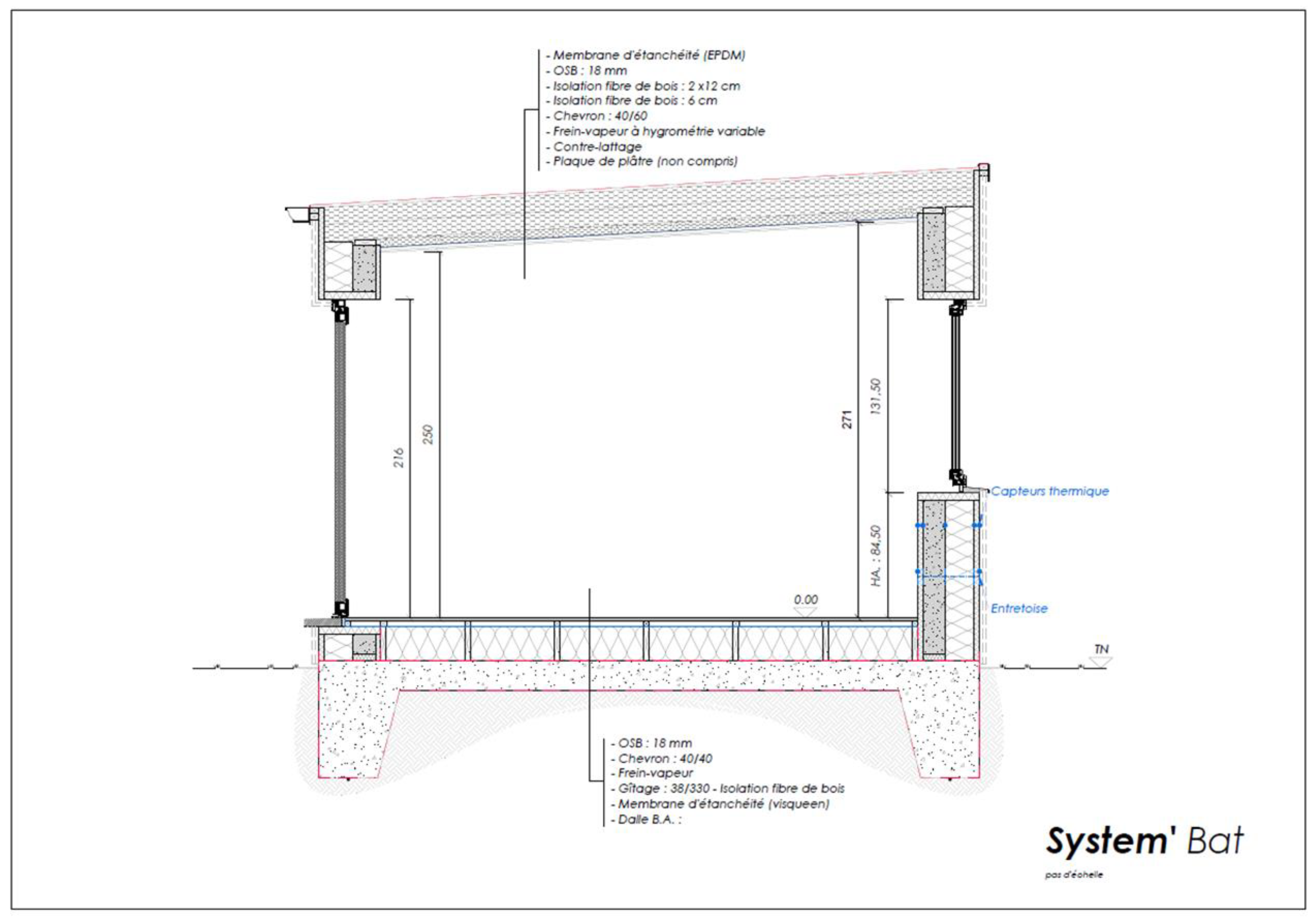
Figure A1. Vertical cut plan of the mono-zone building.
Energies 14 02551 g0a1
Figure A2. Horizontal cut plan of the mono-zone building.
Energies 14 02551 g0a2

References

  1. Zhu, Q.; Xu, X.; Wang, J.; Xiao, F. Development of dynamic simplified thermal models of active pipe-embedded building envelopes using genetic algorithm. Int. J. Therm. Sci. 2014, 76, 258–272. [Google Scholar] [CrossRef]
  2. Soria-Verdugo, A.; Rubio-Rubio, M.; Goos, E.; Riedel, U. Combining the lumped capacitance method and the simplified distributed activation energy model to describe the pyrolysis of thermally small biomass particles. Energy Convers. Manag. 2018, 175, 164–172. [Google Scholar] [CrossRef] [Green Version]
  3. Belmonte, J.F.; Eguía, P.; Molina, A.E.; Almendros-Ibáñez, J.A.; Salgado, R. A simplified method for modeling the thermal performance of storage tanks containing PCMs. Appl. Therm. Eng. 2016, 95, 394–410. [Google Scholar] [CrossRef]
  4. Gao, X.; Liu, J.; Hu, R.; Akashi, Y.; Sumiyoshi, D. A simplified model for dynamic analysis of the indoor thermal environment of rooms with a Chinese kang. Build. Environ. 2017, 111, 265–278. [Google Scholar] [CrossRef]
  5. Al Assaad, D.; Habchi, C.; Ghali, K.; Ghaddar, N. Simplified model for thermal comfort, IAQ and energy savings in rooms conditioned by displacement ventilation aided with transient personalized ventilation. Energy Convers. Manag. 2018, 162, 203–217. [Google Scholar] [CrossRef]
  6. Fine, J.P.; Nguyen, H.V.; Friedman, J.; Leong, W.H.; Dworkin, S.B. A simplified ground thermal response model for analyzing solar-assisted ground source heat pump systems. Energy Convers. Manag. 2018, 165, 276–290. [Google Scholar] [CrossRef]
  7. Gao, J.; Yan, T.; Xu, T.; Ling, Z.; Wei, G.; Xu, X. Development and experiment validation of variable-resistance-variable-capacitance dynamic simplified thermal models for shape-stabilized phase change material slab. Appl. Therm. Eng. 2019, 146, 364–375. [Google Scholar] [CrossRef]
  8. Kharbouch, Y.; Ouhsaine, L.; Mimet, A.; El Ganaoui, M. Thermal performance investigation of a PCM-enhanced wall/roof in northern Morocco. Build. Simul. 2018, 11, 1083–1093. [Google Scholar] [CrossRef]
  9. Wei, T.-W.; Oprins, H.; Cherman, V.; Van der Plas, G.; De Wolf, I.; Beyne, E.; Baelmans, M. Experimental characterization and model validation of liquid jet impingement cooling using a high spatial resolution and programmable thermal test chip. Appl. Therm. Eng. 2019, 152, 308–318. [Google Scholar] [CrossRef]
  10. Habibi Khalaj, A.; Halgamuge, S.K. A Review on efficient thermal management of air- and liquid-cooled data centers: From chip to the cooling system. Appl. Energy 2017, 205, 1165–1188. [Google Scholar] [CrossRef]
  11. Bouguezzi, S.; Ayadi, M.; Ghariani, M. Developing a Simplified Analytical Thermal Model of Multi-chip Power Module. Microelectron. Reliab. 2016, 66, 64–77. [Google Scholar] [CrossRef]
  12. Deb, C.; Schlueter, A. Review of data-driven energy modelling techniques for building retrofit. Renew. Sustain. Energy Rev. 2021, 144, 110990. [Google Scholar] [CrossRef]
  13. Ritzberger, D.; Höflinger, J.; Du, Z.P.; Hametner, C.; Jakubek, S. Data-driven parameterization of polymer electrolyte membrane fuel cell models via simultaneous local linear structured state space identification. Int. J. Hydrogen Energy 2021, 46, 11878–11893. [Google Scholar] [CrossRef]
  14. Chau, T.T.T.; Ailliot, P.; Monbet, V. An algorithm for non-parametric estimation in state–space models. Comput. Stat. Data Anal. 2021, 153, 107062. [Google Scholar] [CrossRef]
  15. Wu, X.; He, H.; Chen, G. A new state-space method for exponentially damped linear systems. Comput. Struct. 2019, 212, 137–144. [Google Scholar] [CrossRef]
  16. Ouhsaine, L.; Ramenah, H.; El Ganaoui, M.; Mimet, A. Dynamic state-space model and performance analysis for solar active walls embedded phase change material. Sustain. Energy Grids Netw. 2020, 24, 100401. [Google Scholar] [CrossRef]
  17. Fateh, A.; Borelli, D.; Spoladore, A.; Devia, F. A State-Space Analysis of a Single Zone Building Considering Solar Radiation, Internal Radiation, and PCM Effects. Appl. Sci. 2019, 9, 832. [Google Scholar] [CrossRef] [Green Version]
  18. Qian, N.; Chang, G. Optimal filtering for state space model with time-integral measurements. Measurement 2021, 176, 109209. [Google Scholar] [CrossRef]
  19. Chen, X.; Wang, Q.; Srebric, J. A data-driven state-space model of indoor thermal sensation using occupant feedback for low-energy buildings. Energy Build. 2015, 91, 187–198. [Google Scholar] [CrossRef]
  20. Yao, Y.; Wang, W.; Huang, M. A state-space dynamic model for vapor compression refrigeration system based on moving-boundary formulation. Int. J. Refrig. 2015, 60, 174–189. [Google Scholar] [CrossRef]
  21. Morsli, S.; Boussoufi, M.; Sabeur, A.; El Ganaoui, M.; Bennacer, R. Small to large scale mixed turbulent convection: Buildings application. Int. J. Numer. Methods Heat Fluid Flow 2018, 28, 188–205. [Google Scholar] [CrossRef]
  22. Kircher, K.J.; Max Zhang, K. On the lumped capacitance approximation accuracy in RC network building models. Energy Build. 2015, 108, 454–462. [Google Scholar] [CrossRef] [Green Version]
  23. Mnasri, F.; Bahria, S.; Slimani, M.E.-A.; Lahoucine, O.; El Ganaoui, M. Building incorporated bio-based materials: Experimental and numerical study. J. Build. Eng. 2020, 28, 101088. [Google Scholar] [CrossRef]
  24. Li, M.; Khelifa, M.; El Ganaoui, M. Mechanical characterization of concrete containing wood shavings as aggregates. Int. J. Sustain. Built Environ. 2017, 6, 587–596. [Google Scholar] [CrossRef]
  25. Ramspeck, C.B.; Jakob, F.E.; Kennedy, S.D.; Knebel, D.E.; Kohloss, F.H.; McBride, M.F.; Modera, M.P.; Nasseri, C.H.; Shavit, G.; Tree, D.R.; et al. ASHRAE STANDARDS COMMITTEE 2003–2004. p. 77. Available online: https://www.google.com.hk/url?sa=t&rct=j&q=&esrc=s&source=web&cd=&ved=2ahUKEwiTqIXstqLwAhVhyYsBHTY-BucQFjAAegQIAxAD&url=http%3A%2F%2Fwww.ditar.cl%2Farchivos%2FNormas_ASHRAE%2FT0080ASHRAE-55-2004-ThermalEnviromCondiHO.pdf&usg=AOvVaw0frR3-OPQO-waPtde0g_w1 (accessed on 21 April 2021).
  26. EnergyPlus Testing with ANSI/ASHRAE Standard 140-2001 (BESTEST). 2004; p. 91. Available online: https://www.google.com.hk/url?sa=t&rct=j&q=&esrc=s&source=web&cd=&ved=2ahUKEwi8_6mtt6LwAhWiIaYKHbOuDXgQFjAAegQIAxAD&url=https%3A%2F%2Fsimulationresearch.lbl.gov%2Fdirpubs%2Fepl_bestest_ash.pdf&usg=AOvVaw3iq8s3M8QeBtRmd0OBbTJo (accessed on 21 April 2021).
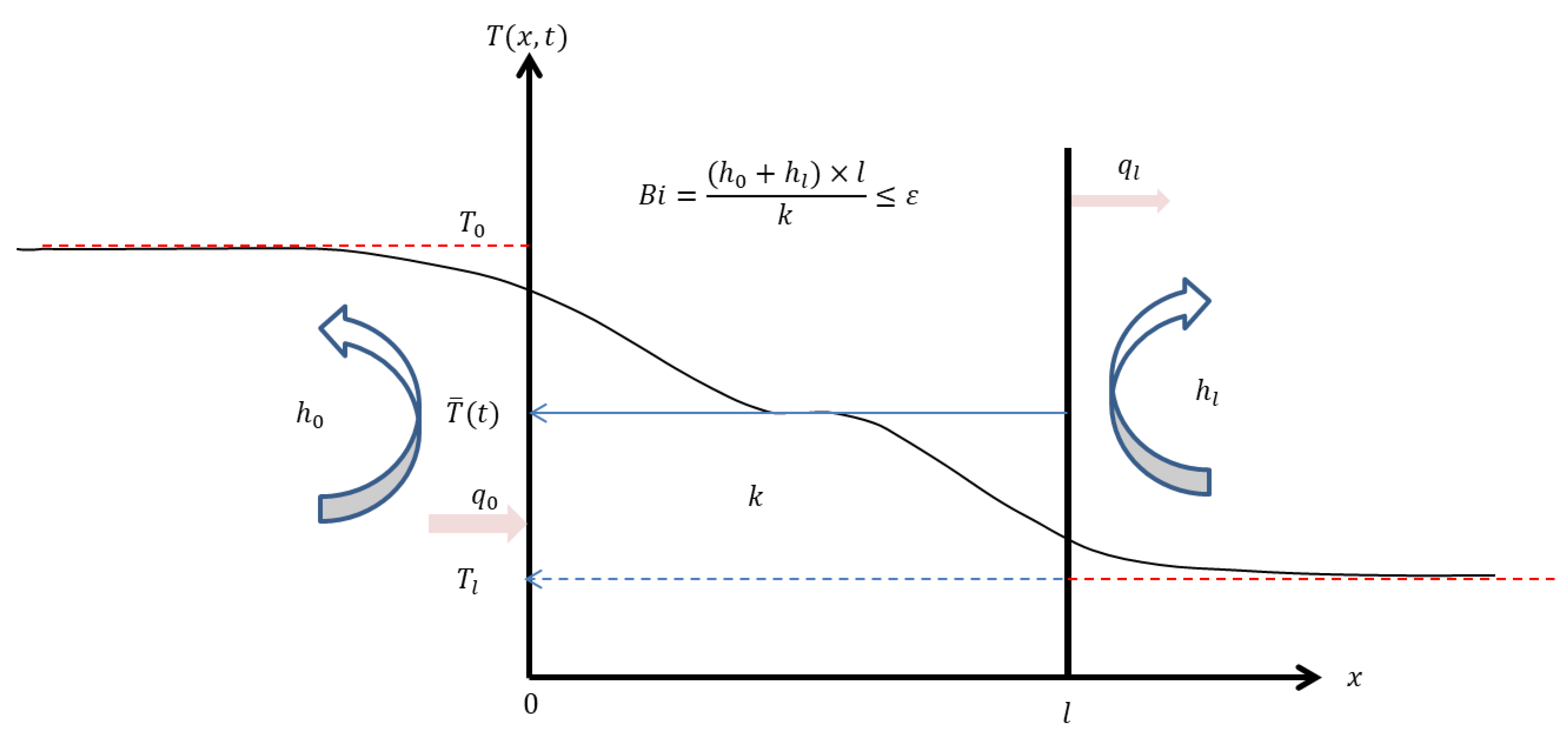
Figure 1. The heat transfer problem presented for a 1D wall.
Energies 14 02551 g001
Figure 2. The substitutive coefficients network scheme.
Energies 14 02551 g002
Figure 3. The eco-cottage building on the Longwy site. (Lorraine University, North East of France, 300 m above the sea level, 49.52° N and 5.769° E). The building plans are given in Appendix F.
Energies 14 02551 g003
Figure 4. The thermal SCN scheme of the mono-zone eco-cottage.
Energies 14 02551 g004
Figure 5. Simplified schematic for the thermal behavior in Physical space vs. Dimensionless space.
Energies 14 02551 g005
Figure 6. Model adjustment by numerical simulation for M = 36.
Energies 14 02551 g006
Figure 7. Temperature dynamics of the internal air and roof layers profiles.
Energies 14 02551 g007
Figure 8. Global solar radiation with internal ambient and floor temperature dynamics profile.
Energies 14 02551 g008
Figure 9. Global solar radiation with ambient and door temperature dynamics profile.
Energies 14 02551 g009
Figure 10. Global solar radiation with ambient and wall layers temperature dynamics profile.
Energies 14 02551 g010
Table 1. The r(q,p) set of state parameters for the model.
Roof LayersWindowsDoorWallsFloor Layers
( q 01 , p 12 ) ( 0.59 ,   1.37 ) ( 0.33 ,   0.66 ) ( 0.56 ,   0.44 ) ( 0.8 ,   2.12 ) ( 0.6 ,   1.23 )
( q 21 , p 23 ) ( 0.59 ,   0.17 ) ( 0.66 ,   0.66 ) ( 0.44 ,   0.44 ) ( 0.2 ,   0.022 ) ( 0.58 ,   0.1 )
( q 32 , p 34 ) ( 0.11 ,   0.25 ) -- ( 0.04 ,   1.5 ) ( 0.02 ,   0.98 )
( q 43 , p 45 ) ( 0.17 ,   0.62 ) -- ( 0.6 ,   0.39 ) ( 0.5 ,   0.5 )
( q 45 , p 56 ) ( 0.85 ,   1.14 ) -- ( 0.84 ,   0.84 ) ( 1 ,   1 )
Publisher’s Note: MDPI stays neutral with regard to jurisdictional claims in published maps and institutional affiliations.