Optimization Method for Operation Schedule of Microgrids Considering Uncertainty in Available Data

Abstract

Operation scheduling in electric power grids is one of the most practical optimization problems as it sets a target for the efficient management of the electric power supply and demand. Advancement of a method to solve this issue is crucially required, especially in microgrids. This is because the operational capability of microgrids is generally lower than that of conventional bulk power grids, and therefore, it is extremely important to develop an appropriate, coordinated operation schedule of the microgrid components. Although various techniques have been developed to solve the problem, there is no established solution. The authors propose a problem framework and a solution method that finds the optimal operation schedule of the microgrid components considering the uncertainty in the available data. In the authors’ proposal, the objective function of the target problem is formulated as the expected cost of the microgrid’s operations. Since the risk of imbalance in the power supply and demand is evaluated as a part of the objective function, the necessary operational reserve power is automatically calculated. The usefulness of the proposed problem framework and its solution method was verified through numerical simulations and the results are discussed.

1. Introduction

Microgrids are a framework of smart power grids that manage a localized group of electrical power sources and loads. They can be operated in both connected and disconnected to the conventional bulk power grid [1,2,3]. Based on the growth in the market penetration of renewable energy sources (RESs), microgrids are now regarded as one of the most practical, sustainable power grids. In fact, many studies and developments in the field of microgrid-related technologies are currently being carried out [4,5], as well as demonstrative field tests [6,7].

There are two types of microgrid components: one is the controllable component, and the other is the uncontrollable one. Controllable power generation systems (CGs), energy storage systems (ESSs), and controllable loads (CLs) are examples of the former. The attributes of the controllable components usually depend on the judgement of whether the power grids accept the reverse power flow from them or not. Electric vehicles (EVs) are a typical example (accepted: ESS, not accepted: CL). In contrast, the latter type consists of electrical appliances on the consumer side and variable renewable energy-based generation systems (VREGs). Since it is difficult for microgrid operators to control electrical appliances, this paper does not include them as a type of CL. In microgrids, the VREGs take a significant portion of the electrical power source, and thus, they create difficulties in the management of the power supply and demand. This is because VREGs, whose outputs are strongly dependent on the weather conditions, introduce additional uncertainty into the readily available data that microgrids must rely on for their operation schedule. If microgrid operators cannot maintain the balance of power supply and demand, the resulting power surplus or shortage leads to significant impacts on activities in our society. Therefore, the surplus or the shortage of the power supply has to be eliminated by extra payments to the bulk power grids. This is an imbalance penalty and it is generally very expensive. For these reasons, the advancement of operation scheduling techniques in microgrids is crucially required.

Focusing on the CGs’ operations, we can formulate operation scheduling problems in microgrids as mixed-integer programming (MIP) problems that combine the optimization problems of the unit commitment (UC) and the economic load dispatch (ELD). These problems are similar to the UC-ELD problems of thermal power generation systems in bulk power grids, and thus, their solution methods are applicable. Historically, branch-and-bound (BB) [8,9] and dynamic programming (DP) [10,11] have been used for the operation scheduling of thermal power generation. Also, there are many studies that have adopted intelligent optimization algorithms as the basis of their solution methods including the application of evolutionary programming (EP) [12], genetic algorithms (GAs) [13], simulated annealing (SA) [14,15], tabu search (TS) [16,17], and particle swarm optimization (PSO) [18,19,20]. Traditional optimization algorithms are difficult to apply to large-scale or complicated problems, while intelligent algorithms cannot guarantee the mathematical optimality of the obtained solution. This is the reason why various algorithms have been applied to the target problems; nevertheless, there is still no established solution method.

Practical operation scheduling problems in microgrids have become more complicated. Since the other controllable components, ESSs and the CLs, have a large influence on the microgrid operations, it is important to examine the state of the charging/discharging operation of the ESSs and the charging (or electricity consumption) of the CLs [21,22,23,24,25]. From the viewpoint of efficient management of the power supply and demand, we must simultaneously treat these states as the optimization variables while considering countermeasures for the influence of the uncertainty [26,27,28].

This paper presents a problem framework and a solution method that finds the optimal coordinated operation schedule for the microgrid components. In the problem formulation, the objective function is represented as the expected cost of the microgrid operations. This feature enables us to deal with the uncertainty in the prediction of the VREG output as a risk of cost increases, and then to automatically secure the necessary operational reserve power. PSO, which is one of the most popular nature-inspired intelligent algorithms, was selected as the basis of the solution method. The trend in the VREG output prediction was treated as a continuous probability density function in the development of the solution method. Finally, the validity of the authors’ proposal was verified through numerical simulations on a microgrid model, and the results are discussed below.

2. Problem Framework

As shown in Figure 1, microgrids generally consist of CGs, ESSs, CLs, electrical loads, and VREGs. Components 1–3 are controllable, and components 4 and 5 are uncontrollable. We can aggregate the latter into one uncontrollable component. This is the net load, and its values are set by the sum of the values of electrical loads and VREG outputs in each time interval. Based on the predicted values of the net load, operation scheduling of the microgrids is represented as the problem of determining a set of start-up/shut-down times and output shares of the CGs, charging/discharging states of the ESSs, and charging states of the CLs.

If the microgrid operators cannot appropriately manage the balance of the power supply and demand, an extra payment is required for additional electricity trading to compensate for the resulting power surplus or shortage; this is the imbalance penalty. The imbalance penalty is normally very expensive, and therefore, microgrid operators secure reserve power to prevent any unexpected payment. On the other hand, the reservation of electrical resources at the operation scheduling stage, e.g., one day ahead, can reduce the difficulties in rescheduling the management of the power supply and demand. In other words, appropriate scheduling of the electricity trade contributes to improving the economic efficiency, reliability, and quality of the power management. Under these circumstances, trading electricity is regarded as an additional controllable factor in this paper, although microgrid operators cannot control components of the bulk power grids.

2.1. Problem Formulation

Microgrid operators design an operation schedule for all controllable components in advance. This problem is formulated as an MIP problem, and its optimization variables are defined as

$$u_{i,t}\in \left\{0, 1\right\},\mathrm{for}\forall i,\forall t,$$

(1)

$$g_{i,t}\in \left[G_i^{\min },G_i^{\max }\right],\mathrm{for}\forall i,\forall t,$$

(2)

$$s_{j,t}\in \left[S_j^{\min },S_j^{\max }\right],\mathrm{for}\forall j,t\in T_j^{\prime },$$

(3)

$$e_t\in ℝ,\mathrm{for}\forall t,$$

(4)

where $t$ is time ($t=1,\cdots ,T$); $i$ is the number assigned to the CGs ($i=1,\cdots ,NG$); $u_{i,t}$ is the ON/OFF state variable of CG $i$ (ON: $1$, OFF: $0$), which is an element of vectors $u_t$ and $u$; $g_{i,t}$ is the output of CG $i$, which is an element of vectors $g_t$ and $g$; $G_i^{\max }$ and $G_i^{\min }$ are the maximum and the minimum outputs of CG $i$; $j$ is the number assigned to the ESSs ($j=1,\cdots ,NS$); $s_{j,t}$ is the output of ESS $j$, which is an element of vectors $s_t$ and $s$; $S_j^{\max }$ and $S_j^{\min }$ are the maximum and the minimum capable outputs of ESS $j$ ($S_j^{\min }\le 0\le S_j^{\max }$); $T_j^{\prime }$ is the set of periods that the ESSs are available; $e_t$ is the trading electricity, which is an element of vector $e$.

In this paper, the CLs are regarded as a type of ESS, and their states are treated by Equation (3) by substituting $S_j^{\max }$ with zero.

The traditional problem frameworks often require accurate data for the uncontrollable components, which is impractical in the actual operation scheduling of the microgrids. The only available data are the predicted values of these components with the uncertainty. Here, we define the net loads as the stochastic variables and set their likely ranges as

$${\tilde{d}}_t\in \left[d_t^{\min },d_t^{\max }\right],\mathrm{for}\forall t,$$

(5)

where ${\tilde{d}}_t$ is the predicted net loads, which is an element of vector $\tilde{d}$; $d_t^{\max }$ and $d_t^{\min }$ are the maximum or the minimum values of the assumed net loads.

The operation scheduling problem is to determine the set of $\left(u,g,s,e\right)$ in terms of minimizing the sum of the operational costs of the microgrid components. Fuel costs of the CGs are usually approximated as quadratic functions by means of their outputs, and these can be reduced by steady control of the CG outputs. As opposed to the CGs, the ESSs do not directly consume fuel, and this brings new challenges to the evaluation of the ESS operations. Based on Equation (5), the objective function is represented as

$$\underset{u,g,s,e}{\min }E\left[f\left(u,g,s,e,\tilde{d}\right)\right],$$

(6)

$$E\left[f\left(u,g,s,e,\tilde{d}\right)\right]={{\displaystyle \sum }}_{t=1}^T\left\{{{\displaystyle \int }}_{d_t^{\min }}^{d_t^{\max }}\left(f_1+f_3\right)·p\left(d_t^{†}\right)\mathrm{d}{d}_t^{†}+f_2\right\},$$

(7)

$$f_1={{\displaystyle \sum }}_{i=1}^{NG}\left\{(A_i+B_i{g}_{i,t}^{†}+C_i·{\left(g_{i,t}^{†}\right)}^2)·u_{i,t}\right\},$$

(8)

$$f_2={{\displaystyle \sum }}_{i=1}^{NG}\left\{D_i·u_{i,t}\left(1-u_{i,t-1}\right)\right\},$$

(9)

$$f_3=M_t{e}_t+VI{O}_t·\left({{\displaystyle \sum }}_{i=1}^{NG}{g}_{i,t}^{†}{u}_{i,t}+{{\displaystyle \sum }}_{j=1}^{NS}{s}_{j,t}+e_t-d_t^{†}\right),$$

(10)

where $d_t^{†}$ is the realization values of net loads; $g_{i,t}^{†}$ is the CG outputs calculated according to $d_t^{†}$; $p( )$ is the probability density function; $A_i$, $B_i$, and $C_i$ are the coefficients of fuel cost of CG $i$; $D_i$ is the start-up cost of CG $i$; $M_t$ is the price of electricity trade in operation scheduling stage; $VI{O}_t$ is the price of the imbalance penalty.

As shown in Equation (10), ESSs contribute to reducing the operational cost of CGs and the payment for trading electricity.

The microgrid components must satisfy the following constraints:

• State of duration of the CGs

  $$\mathrm{If}0<u_{i,t}^{on}<U{T}_i\mathrm{then}{u}_{i,t}=1;\mathrm{If}0<u_{i,t}^{off}<D{T}_i\mathrm{then}{u}_{i,t}=0,\mathrm{for}\forall i,\forall t,$$

  (11)

  where $u_{i,t}^{\mathrm{on}}$ and $u_{i,t}^{\mathrm{off}}$ are the consecutive operating and suspended duration of CG $i$, and $U{T}_i$ and $D{T}_i$ are the minimum operating and suspended duration of CG $i$, respectively.
• Ramp rate of the CGs

  $$\mathsf{\Delta }{G}_i^{\mathrm{down}}\le g_{i,t}-g_{i,t-1}\le \mathsf{\Delta }{G}_i^{\mathrm{up}},\mathrm{for}\forall i,\forall t,$$

  (12)

  where $\mathsf{\Delta }{G}_i^{\mathrm{up}}$ and $\mathsf{\Delta }{G}_i^{\mathrm{down}}$ are the ramp-up and the ramp-down rates of CG $i$.
• Output range of the CGs

  $$\begin{gathered} g_{i,t}^{\min }\le g_{i,t}\le g_{i,t}^{\max },\mathrm{for}\forall i,\forall t. \\ (g_{i,t}^{\max }=\min \left(G_i^{\max },g_{i,t-1}+\mathsf{\Delta }{G}_i^{\mathrm{up}}\right);g_{i,t}^{\min }=\max \left(G_i^{\min },g_{i,t-1}+\mathsf{\Delta }{G}_i^{\mathrm{down}}\right).) \end{gathered}$$

  (13)
• State of charge (SOC) of the ESSs

  $$\begin{gathered} Q_j^{\min }\le q_{j,t}\le Q_j^{\max },\mathrm{for}\forall j,t\in T_j^{\prime }, \\ (\mathrm{If}{s}_{j,t}>0\mathrm{then}{q}_{j,t}=q_{j,t-1}-\frac{1}{{\eta }_j}{s}_{j,t};\mathrm{if}{s}_{j,t}<0\mathrm{then}{q}_{j,t}=q_{j,t-1}-{\eta }_j{s}_{j,t}.) \end{gathered}$$

  (14)

  where $q_{j,t}$ is the SOC level of the ESS $j$;$Q_j^{max}$ and $Q_j^{min}$ are the maximum and the minimum SOC levels of the ESS $j$; ${\eta }_j$ is the overall efficiency of the ESS $j$.
• Output range of the ESSs

  $$\begin{gathered} s_{j,t}^{\min }\le s_{j,t}\le s_{j,t}^{\max },\mathrm{for}\forall j,t\in T_j^{\prime }. \\ (s_{i,t}^{\max }=\max \left(S_j^{\max },{\eta }_j\left(Q_j^{\max }-q_{j,t-1}\right)\right);s_{i,t}^{\min }=\min \left(S_j^{\min },\frac{1}{{\eta }_j}\left(q_{j,t-1}-Q_j^{\min }\right)\right).) \end{gathered}$$

  (15)

If the time interval $\mathsf{\Delta }t$, the ramp-up rate $\mathsf{\Delta }{G}_i^{\mathrm{up}}$, and the ramp-down rate $\mathsf{\Delta }{G}_i^{\mathrm{down}}$ satisfy conditions (16) and (17), the constraints (11) and (12) become inactive [20,25]. Similarly, evaluation of the variables $g_{i,t}^{\max }$ and $g_{i,t}^{\min }$ is unnecessary in Equation (13). In this case, $g_{i,t}^{\max }$ and $g_{i,t}^{\min }$ become equal to $G_i^{\max }$ and $G_i^{\min }$, respectively, and this constraint can be integrated into Equation (2).

$$\mathsf{\Delta }t\ge U{T}_i+D{T}_i,\mathrm{for}\forall i,$$

(16)

$$\mathsf{\Delta }{G}_i^{\mathrm{up}}\ge G_i^{\max }-G_i^{\min };\mathsf{\Delta }{G}_i^{\mathrm{down}}\le G_i^{\min }-G_i^{\max },\mathrm{for}\forall i.$$

(17)

Since these conditions are satisfied in the operation scheduling stage of the microgrids, the authors ignore the constraints (11) and (12) and treat the constraint (13) as the same as Equation (2).

2.2. Characteristics of Proposed Problem Framework

The formulated problem is to determine the optimal operation schedule, that is the set of $\left(u^{*},g^{*},s^{*},e^{*}\right)$. There are two types of optimization variables: $u$ is the set of discrete variables, and the others are sets of continuous variables. Moreover, we cannot omit the influence of the ESSs and the CLs from the microgrid operations because their capacities are large in regard to their share of electrical power sources. These are the reasons why the target problem is complicated as compared to that of the bulk power grids.

As shown in Equations (6)–(10), the objective function is formulated as the expected operational cost of the microgrids. Equations (7) and (10), evaluate the impact of the unexpected imbalance as a potential risk of operational cost increases. In the process, the reserve power is evaluated corresponding to the risk of a cost increase. Hence, we can remove the traditional constraints for the balance of power supply and demand and the operational margin from the problem formulation. These are integrated into the objective function.

3. Solution Method

In conventional approaches [29,30], the calculation of Equation (7) is often replaced with an iterative calculation using discrete probability distributions of the past VREG outputs. The results of this calculation strongly depends on the number and the variety of samples in the past record. Too small a sample number produces inaccuracy in the calculation results, while a larger number increases the costs of the iterative calculation. The authors propose a strategy enabling us to treat $p\left(d_t^{†}\right)$ as a continuous function, and then apply PSO to the target problem framework.

3.1. Approximation of Outputs of Controllable Generation Systems

As shown in Equation (8), shape of the fuel cost function depends on the operating CGs, and economic output share of the operating CGs is determined by the fuel cost coefficients of each CG. In the proposed solution method, first, possible UC candidates are enumerated exactly. As opposed to bulk power grids, the number of CGs in microgrids is sufficiently small, and thus we can identify all possible UC candidates. Next, the optimal output share of the operating CGs is calculated in association with the enumerated UC candidates. Since the ELD problems become a quadratic programming problem by fixing the values of $u_{i,t}$, quadratic programming solvers are applicable in this step. Finally, by nonlinear regression, each set of optimal output shares are approximated as the aggregated fuel cost functions of the UC candidates. Through this process, we can replace Equation (13) with (18), and then Equation (8) with (19).

$$\begin{gathered} h_t^{\min }\le h_t\le h_t^{\max },\mathrm{for}\forall t, \\ (h_t^{\max }={{\displaystyle \sum }}_{i=1}^{NG}{G}_i^{\max }{u}_{i,t};h_t^{\min }={{\displaystyle \sum }}_{i=1}^{NG}{G}_i^{\min }{u}_{i,t}.) \end{gathered}$$

(18)

$$f_1^{\prime }=A_{u_t}^{\prime }+B_{u_t}^{\prime }{h}_t^{†}+C_{u_t}^{\prime }·{\left(h_t^{†}\right)}^2,$$

(19)

where $h_t$ is the sum of outputs of the operating CGs ($={{\displaystyle \sum }}_{i=1}^{NG}{g}_{i,t}{u}_{i,t}$); $h_t^{†}$ is the sum of operating CG outputs calculated according to $d_t^{†}$; $A_{u_t}^{\prime }$, $B_{u_t}^{\prime }$, and $C_{u_t}^{\prime }$ are the coefficients of approximated fuel cost associated with the vector $u_t$.

Table 1. Specifications of CGs (“¥” means “any currency unit is applicable”).

$\mathit{i}$	${\mathit{A}}_{\mathit{i}}(\yen )$	${\mathit{B}}_{\mathit{i}}(\yen /\mathbf{MW})$	${\mathit{C}}_{\mathit{i}}(\yen /{\mathbf{MW}}^2)$	${\mathit{D}}_{\mathit{i}}(\yen )$	${\mathit{G}}_{\mathit{i}}^{\mathbf{max}}\left(\mathbf{MW}\right)$	${\mathit{G}}_{\mathit{i}}^{\mathbf{min}}\left(\mathbf{MW}\right)$
1	14,000	8500	60	3000	20.0	4.0
2	7800	6000	90	1000	16.0	3.2
3	2400	4000	100	500	12.0	2.4

summarizes the specifications of sample CGs, and Figure 2 displays their fuel cost functions. These were formulated by referring to [18,20,25,30]. When we focus on microgrids with three CGs, the possible UC candidates are $\left(0,0,0\right)$, $\left(0,0,1\right)$, $\left(0,1,0\right)$, $\left(1,0,0\right)$, $\left(0,1,1\right)$, $\left(1,0,1\right)$, $\left(1,1,0\right)$, and $\left(1,1,1\right)$. However, we can remove $\left(0,0,0\right)$–$\left(1,0,0\right)$ from the approximation target because their optimal output shares are obvious. Quadratic programming calculates the optimal output shares for each of the UC candidates $\left(0,1,1\right)$–$\left(1,1,1\right)$, and they are independently approximated by the nonlinear regression. Figure 3 illustrates the fuel cost functions of the aggregated operating CGs. As a result, we can obtain the coefficients $A_{u_t}^{\prime }$, $B_{u_t}^{\prime }$, and $C_{u_t}^{\prime }$ as summarized in

Table 2. Calculated coefficients in Figure 3 (“¥” means “any currency unit is applicable”).

${\mathit{u}}_{\mathit{t}}$	${\mathit{A}}_{{\mathit{u}}_{\mathit{t}}}^{\prime }\left(\right)$	${\mathit{B}}_{{\mathit{u}}_{\mathit{t}}}^{\prime }(\yen /\mathbf{MW})$	${\mathit{C}}_{{\mathit{u}}_{\mathit{t}}}^{\prime }(\yen /{\mathbf{MW}}^2)$
(0,1,1)	18,264	3383	101
(1,0,1)	37,381	2558	154
(1,1,0)	30,689	5767	75
(1,1,1)	48,746	3254	85

.

The proposed approximation can be completed as a preprocessing of the operation scheduling problem using readily available information, but it is applicable only when the microgrid does not have so many CGs. For example, with 10 CGs, the number of possible UC candidates is 2¹⁰ (= 1024). In addition, its results are strongly dependent on the specifications of the CGs. However, there was no significant difference in the pre-calculation results of the widely used power grid models, e.g., IEEE 118 bus model [31,32]. Through simple verification, the authors concluded that this approximation is normally applicable to microgrids.

3.2. Reformulation of Objective Function

Before reformulating the objective function, the authors introduced a new variable ${\epsilon }_t$ and replaced the stochastic variables as

$${\epsilon }_t=d_t-\left({{\displaystyle \sum }}_{j=1}^{NS}{s}_{j,t}+e_t\right),$$

(20)

$$\begin{gathered} \widetilde{{\epsilon }_t}\in \left[{\epsilon }_t^{\min },{\epsilon }_t^{\max }\right],\mathrm{for}\forall t. \\ ({\epsilon }_t^{\max }=d_t^{\max }-\left({{\displaystyle \sum }}_{j=1}^{NS}{s}_t+e_t\right);{\epsilon }_t^{\min }=d_t^{\min }-\left({{\displaystyle \sum }}_{j=1}^{NS}{s}_t+e_t\right).) \end{gathered}$$

(21)

Then, based on Equations (18)–(21), function (7) is reformulated as

$$E\left[f\left(u,g,s,e,\tilde{\epsilon }\right)\right]={{\displaystyle \sum }}_{t=1}^T\left\{{{\displaystyle \int }}_{{\epsilon }_t^{\min }}^{{\epsilon }_t^{\max }}\left(f_1^{\prime }+f_3^{\prime }\right)·p\left({\epsilon }_t^{†}\right)\mathrm{d}{\epsilon }_t^{†}+f_2\right\}.$$

(22)

$$\begin{gathered} \mathrm{If}{h}_t^{\max }<{\epsilon }_t^{†}\mathrm{then} \\ {f}_1^{\prime }=A_{u_t}+B_{u_t}{h}_t^{\max }+C_{u_t}·{\left(h_t^{\max }\right)}^2;f_3^{\prime }=M_t{e}_t+VI{O}_t·\left({\epsilon }_t^{†}-h_t^{\max }\right). \end{gathered}$$

(23)

$$\begin{gathered} \mathrm{If}{h}_t^{\min }\le {\epsilon }_t^{†}\le h_t^{\max }\mathrm{then} \\ {f}_1^{\prime }=A_{u_t}+B_{u_t}{\epsilon }_t^{†}+C_{u_t}·{\left({\epsilon }_t^{†}\right)}^2;f_3^{\prime }=M_t{e}_t. \end{gathered}$$

(24)

$$\begin{gathered} \mathrm{If}{\epsilon }_t^{†}<h_t^{\min }\mathrm{then} \\ {f}_1^{\prime }=A_{u_t}+B_{u_t}{h}_t^{\min }+C_{u_t}·{\left(h_t^{\min }\right)}^2;f_3^{\prime }=M_t{e}_t+VI{O}_t·\left(h_t^{\min }-{\epsilon }_t^{†}\right). \end{gathered}$$

(25)

In the case where we set $s_t$ and $e_t$ by any means, the probability density function $p\left({\epsilon }_t^{†}\right)$ in Equation (22) is a horizontally shifted function of $p\left(d_t^{†}\right)$ in (7).

In the original formulation, the function $\left(f_1+f_3\right)$ is determined by the set of $\left(u_{i,t},g_{i,t},s_{j,t},e_t\right)$, and it is impossible to specify its shape in the range of $\left[{\epsilon }_t^{\min },{\epsilon }_t^{\max }\right]$. Therefore, the integral calculus was replaced with an iterative calculation using discrete probability distributions. On the other hand, in Equation (22), the function $\left(f_1^{\prime }+f_3^{\prime }\right)$ becomes a set of continuous function depending on $\left(u_{i,t},s_{j,t},e_t\right)$ once the process of 3.1 is completed. As a result, we can directly treat the calculation of Equation (22) as an integral calculus.

3.3. Application of Particle Swarm Optimization

By applying the process described in Section 3.1 and Section 3.2, the CG outputs $g_{i,t}$ (or $h_t$) are removed from the optimization variables. However, the target problem is still extremely difficult to solve exactly. In this paper, a PSO was selected as the basis of the solution method.

The standard PSO is the typical population-based stochastic algorithm that iteratively searches the solution space while improving a given measure of solution quality [33], which is the fitness function. An initial set of randomly generated solutions, which is the initial swarm, propagates in the search space towards the globally optimal solution until a termination condition is met. During the process, all members of the swarm fit and share the information of the search space. Each particle $k$ ($k=1,2,\dots ,K$) has a position $x_k^n$ and a velocity $v_k^n$ in the iteration $n$ ($n=1,2,\dots ,N$), and these are updated as

$$x_k^n=x_k^{n-1}+v_k^n,$$

(26)

$$v_k^{n+1}=\omega v_k^n+{\theta }_1{r}_1\left[x_k^{*}-x_k^n\right]+{\theta }_2{r}_2\left[\left(\underset{k}{\min }{x}_k^{*}\right)-x_k^n\right],$$

(27)

where $\omega$ is the inertia weight factor that controls the iteration size; ${\theta }_1$ and ${\theta }_2$ are the cognitive factors that represent the trust for each particle and the swarm; $r_1$ and $r_2$ are the random numbers in the range of $\left[0, 1\right]$; $x_k^{*}$ is the personal best for the particle $k$ (pbest); $\underset{k}{\min }{x}_k^{*}$ is the best in the swarm (gbest).

That is, the particles fly through the search space based on Equations (26) and (27) to find the globally best location.

According to the problem formulation, the fitness function is represented by Equation (22), and the position of the particles is defined as

$$x_k^n={\left(u,s,e\right)}_k^n,\mathrm{for}\forall k,\forall n.$$

(28)

The standard PSO is successful in solving many continuous problems; however, there are still difficulties in the treatment of discrete optimization problems [34]. Therefore, a strategy of binary particle swarm optimization (BPSO) was applied to the proposed solution method as shown below:

$$\mathrm{If}0.5<\frac{1}{1+e^{-u_{i,t}}}\mathrm{then}{u}_{i,t}=1,\mathrm{else}{u}_{i,t}=0,\mathrm{for}\forall i,\forall t.$$

(29)

In (29), the CG $i$ becomes ON at time $t$ if the value of the sigmoid limiting transformation function is greater than or equal to 0.5, otherwise it becomes OFF.

4. Numerical Simulations

With a view to verifying the validity of the authors’ proposal, numerical simulations were carried out on the microgrid model illustrated in Figure 1. The microgrid components were set as three CGs, two aggregated ESSs (one aggregated stationary ESS and one aggregated CL), one aggregated electrical load, and one aggregated VREG. In the numerical simulations, photovoltaic generation systems (PVs) were selected as the VREG. As for the probability density function, the authors used a Laplace distribution whose location parameter was set to the predicted net load, and the scale parameter was set to 1 [35]. The specifications of the CGs are already summarized in Table 1 and Figure 2.

Table 3. Specifications of aggregated ESS and aggregated CL.

ESS				CL
$S_1^{\max }$ (MW)	$S_1^{\min }$ (MW)	$Q_1^{\max }$ (MWh)	$Q_1^{\min }$ (MWh)	$S_2^{\max }$ (MW)	$S_2^{\min }$ (MW)	$Q_2^{\max }$ (MWh)	$Q_2^{\min }$ (MWh)
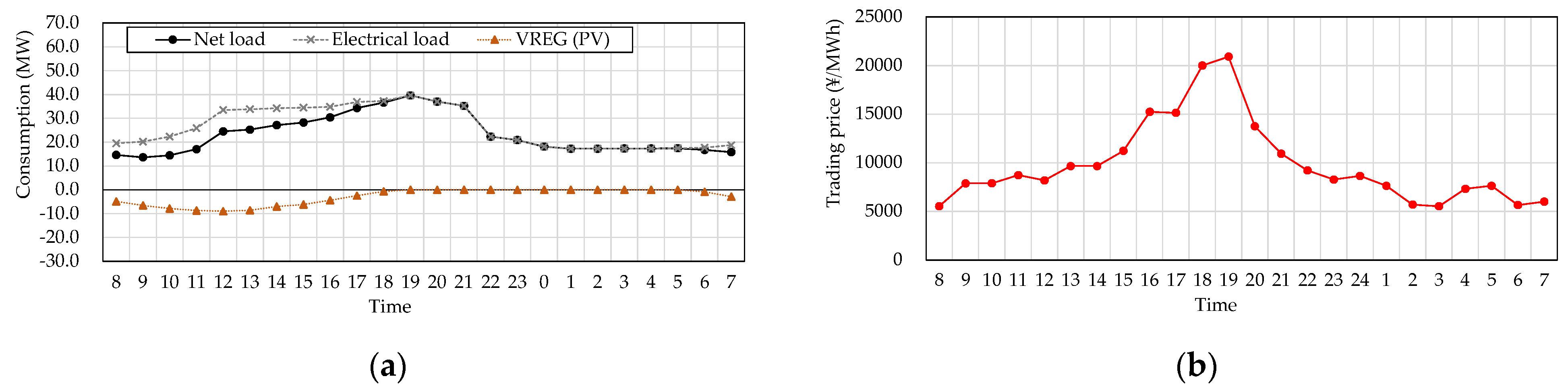
1.8	−1.8	10.4	2.6	0	−1.5	9.6	2.4

shows the specifications of the aggregated ESSs. Profiles of the predicted net load and the price for traded electricity are displayed in Figure 4. These were made with reference to [20,25,30].

The time interval $\mathsf{\Delta }t$ was set to 1 h, and the daily operation schedule ($t=1,2,\dots ,24$) was set as the optimization target. Here, the target period was set from 8:00 ($t=1$) to 7.00 of the next day ($t=24$) considering operation of the CLs. The available duration of the aggregated CL was set from 21:00 ($t=14$) to 7:00 ($t=24$). The initial SOC level of the aggregated ESS was set to 50% of its capacity, and it had to be returned to the original level until the end of the scheduling period. On the other hand, the initial SOC level of the aggregated CL was set to 50%, and it had to be 100% at the end of the scheduling period. In other words, the optimal operation schedule must satisfy the following additional constraints:

$$s_{1,1}=s_{1,24}=0.5Q_1^{\max }.$$

(30)

$$s_{2,1}=0.5Q_2^{\max };s_{2,24}=1.0Q_2^{\max }.$$

(31)

According to the preliminary trial and errors, the parameters of the PSO were set as the following: the total number of particles $K$ was 40; the maximum iteration $N$ was 300; the inertia weight factor was 0.9, and the cognitive factors ${\theta }_1$ and ${\theta }_2$ were 2.0 in both.

Under these conditions, the authors determined the optimal operation schedule of the microgrid. For comparison, the traditional operation schedule was also determined under the assumption that the microgrid operators trusted the predicted data as the basis of the operation scheduling. In the traditional problem framework, the operational cost based on the predicted net load was used as the objective function. Furthermore, the authors assumed that the reserve power must compensate for a deviation within 5% of the predicted net load because the traditional framework requires a constraint for the operational margin.

4.1. Numerical Simulation Results

Figure 5 and Figure 6 illustrate the obtained operation schedules, and their results are summarized in

Table 4. Comparison of numerical simulation results (“¥” means “any currency unit is applicable”).

Problem Framework	Cost using Predicted Net Load (¥)	Expected Cost (¥)
Proposed framework	3,471,260	3,446,339
Traditional framework	3,281,649	3,605,541

.

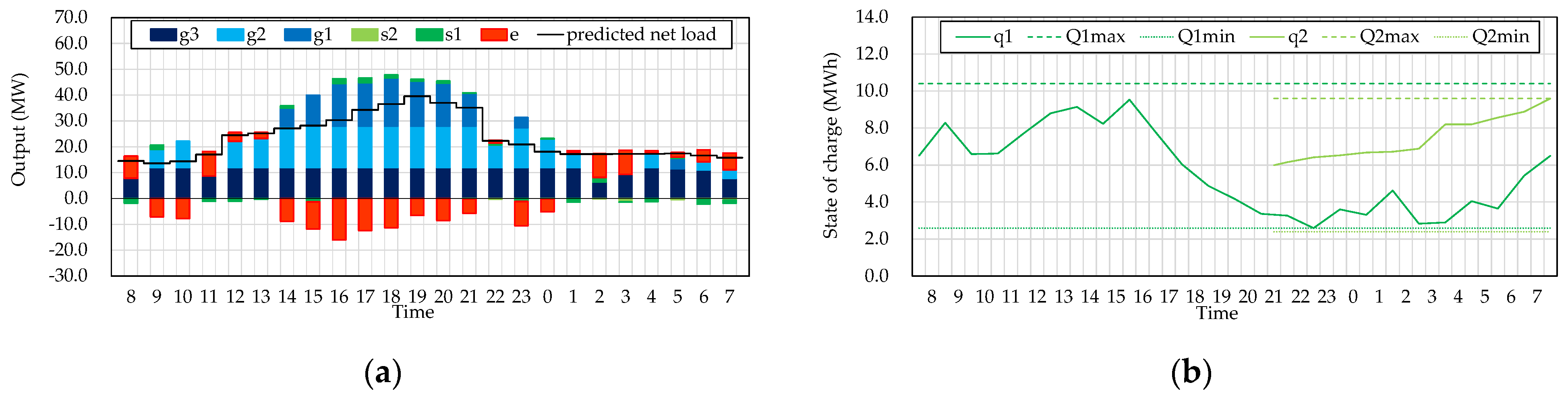
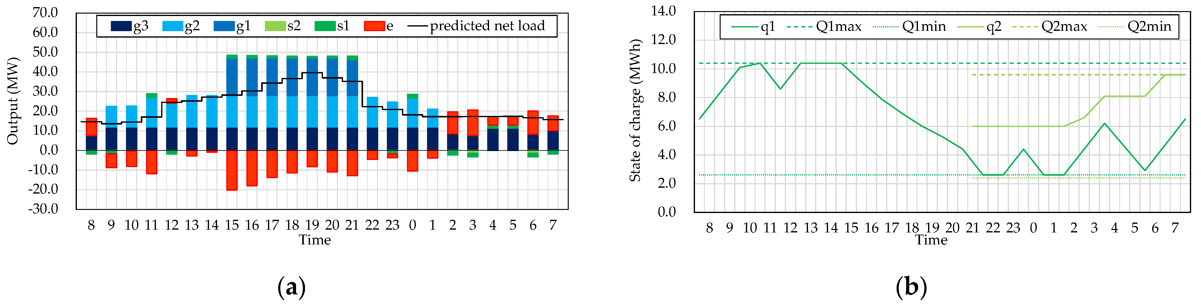
As shown in both Figure 5 and Figure 6, the balance of power supply and demand on the predicted net load was maintained by the coordinated operation of the CGs, the aggregated ESSs, and the electricity trade. As shown in Table 4, if the accuracy of the net load prediction is sufficiently high, the optimal schedule according to the traditional problem framework is better than that of the proposed one. However, this condition is impractical in actual microgrid operations. In contrast, the proposed framework obtained a better solution from the viewpoint of the expected operational cost. Moreover, the difference between the cost using the predicted net load and the expected cost was remarkably small compared to that in the traditional one. This indicates that the optimal operation schedule of the proposed framework generated resilience in the microgrid operations.

These results were obtained within a few minutes on Intel Core i7-8700K @ 3.70 GHz. Therefore, the authors concluded that the proposed solution method is applicable to actual operation scheduling.

4.2. Discussion on Numerical Simulation Results

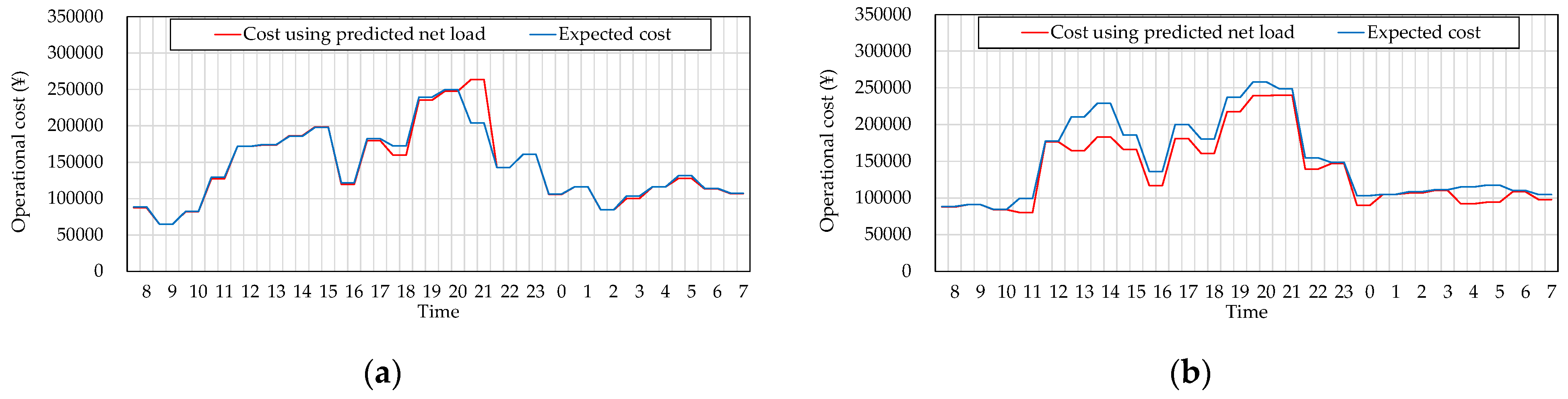
As described in Section 2.2, the necessary reserve power was automatically calculated in the proposed problem framework. Figure 7 shows the differences between the operational margins in Figure 5 and Figure 6. Figure 8 illustrates the transitions of the objective functions.

In Figure 7, the proposed framework enhanced the upper-side margin remarkably from 13:00 to 15:00 and after 22:00. With reference to Figure 7, it can be confirmed that neighboring periods include the peak of the PV output or rapid change in the net load. In general, these conditions lead to difficulty in balancing the operation of power supply and demand. As a result, as shown in Figure 8b, the expected cost was large in comparison with the cost using the predicted net load during the periods. Besides, the cost transitions in Figure 8a were similar, while the transitions in Figure 8b were different. Figure 8b shows that the transition of the expected cost was usually larger than that of the cost using the predicted net load. These results show that the necessary reserve power was automatically secured (in Figure 8), corresponding to the risk of increases in operational costs. Therefore, we can conclude that our proposal functioned well.

5. Conclusions

The authors proposed a problem framework and a solution method that finds the optimal coordinated operation schedule of the microgrid components. In the problem formulation, the objective function was represented as the expected cost of the microgrid operations. Since the operational margin has a large impact on the expected cost, the necessary reserve power is automatically secured in the obtained operation schedule. As a result, we can remove the traditional constraints for the balance of power supply and demand and the operational margin from the problem formulation. In the numerical simulation results, it was confirmed that the proposed objective function made it possible to evaluate the uncertainty in the prediction of the VREG output as the potential risk of cost increases. Meanwhile, the proposed solution method enabled us to treat the trend in VREG output prediction as a continuous probability density function. This indicates that there is no need to be concerned about the number and the variety of samples of the past VREG output in the proposed solution method. Through the numerical simulations and discussion of their results, we were able to conclude that the proposed strategy did not have any significant influence on the process of the solution evaluation and it provided a useful operation schedule.

In future work, the authors will improve the solution method, including a discussion on the appropriate selection of its basis. In addition, the influence ofapproximating the CG outputs will be analyzed in more detail.

References

- Hatziargyriou, N.; Asano, H.; Iravani, R.; Marnay, C. Microgrids. IEEE Power Energy Mag. 2007, 5, 78–94. [Google Scholar] [CrossRef]
- Office of Electricity Delivery and Energy Reliability. DOE Microgrid Workshop Report. Summary Report 2012. Available online: https://www.energy.gov/sites/prod/files/Microgrid%20Workshop%20Report%20August%202011.pdf (accessed on 31 March 2021).
- Ton, D.T.; Smith, M.A. The U.S. Department of Energy’s Microgrid Initiative. Electr. J. 2012, 25, 84–94. [Google Scholar] [CrossRef]
- Liu, C.C.; McAuthur, S.; Lee, S.J. Smart Grid Handbook, 3 Volume Set; John Wiley & Sons: Hoboken, NJ, USA, 2016. [Google Scholar]
- Bevrani, H.; Francois, B.; Ise, T. Microgrid Dynamics and Control; John Wiley & Sons: Hoboken, NJ, USA, 2017. [Google Scholar]
- Investigating R&D Committee on Advanced Power System. Current Status of Advanced Power Systems including Microgrid and Smartgrid. IEEJ Tech. Rep. 2011, 1229. Available online: https://www.bookpark.ne.jp/cm/ieej/detail.asp?content_id=IEEJ-GH1229-PRT (accessed on 31 March 2021). (In Japanese).
- New Energy and Industrial Technology Development Organization. Case Studies of Smart Community Demonstration Project. Available online: http://www.nedo.go.jp/english/reports_20130222.html (accessed on 31 March 2021).
- Cohen, A.I.; Yoshimura, M. A branch-and-Bound Algorithm for Unit Commitment. IEEE Trans. Power Syst. 1983, 102, 444–451. [Google Scholar] [CrossRef]
- Chen, C.L.; Wang, S.C. Branch-and-Bound Scheduling for Thermal Generating Units. IEEE Trans. Energy Convers. 1993, 8, 184–189. [Google Scholar] [CrossRef]
- Snyder, W.L.; Powell, H.D.; Raiburn, J.C. Dynamic Programming Approach to Unit Commitment. IEEE Trans. Power Syst. 1987, 2, 339–348. [Google Scholar] [CrossRef]
- Ouyang, Z.; Shahidehpour, S.M. An Intelligent Dynamic Programming for Unit Commitment Application. IEEE Trans. Power Syst. 1991, 6, 1203–1209. [Google Scholar] [CrossRef]
- Juste, K.A.; Kita, H.; Tanaka, E.; Hasegawa, J. An Evolutionary Programming Solution to the Unit Commitment Problem. IEEE Trans. Power Syst. 1990, 14, 1452–1459. [Google Scholar] [CrossRef]
- Kazarlis, S.A.; Bakirtzis, A.G.; Petridis, V. A Genetic Algorithm Solution to the Unit Commitment Problem. IEEE Trans. Power Syst. 1996, 11, 83–92. [Google Scholar] [CrossRef]
- Mantawy, A.H.; Abdel-Magid, Y.L.; Selim, S.Z. A Simulated Annealing Algorithm for Unit Commitment. IEEE Trans. Power Syst. 1998, 13, 197–204. [Google Scholar] [CrossRef]
- Simopoulos, D.N.; Kavatza, S.D.; Vournas, C.D. Unit Commitment by an Enhanced Simulated Annealing Algorithms. IEEE Trans. Power Syst. 2006, 21, 68–76. [Google Scholar] [CrossRef]
- Rajan, C.C.A.; Mohan, M.R. An Evolutionary Programming-Based Tabu Search Method for Solving the Unit Commitment Problem. IEEE Trans. Power Syst. 2004, 19, 577–585. [Google Scholar] [CrossRef]
- Takano, H.; Zhang, P.; Murata, J.; Hashiguchim, T.; Goda, T.; Iizaka, T.; Nakanishi, Y. A Determination Method for the Optimal Operation of Controllable Generators in Micro Grids that Copes with Unstable Outputs of Renewable Energy Generation. Electr. Eng. Jpn. 2015, 190, 56–65. [Google Scholar] [CrossRef]
- Hayashi, Y.; Miyamoto, H.; Matsuki, J.; Iizuka, T.; Azuma, H. Online Optimization Method for Operation of Generators in Micro Grid. IEEJ Trans. Power and Energy 2008, 128, 388–396. (In Japanese) [Google Scholar] [CrossRef]
- Jeong, Y.W.; Park, J.B. A New Quantum-Inspired Binary PSO: Application to Unit Commitment Problem for Power Systems. IEEE Trans. Power Syst. 2010, 25, 1486–1495. [Google Scholar] [CrossRef]
- Takano, H.; Goto, R.; Soe, T.Z.; Tuyen, N.D.; Asano, H. Operation Scheduling Optimization for Microgrids Considering Coordination of Their Components. Future Internet 2019, 11, 223. [Google Scholar] [CrossRef]
- Lu, B.; Shahidehpour, M. Short-Term Scheduling of Battery in a Grid-Connected PV/Battery System. IEEE Trans. Power Syst. 2005, 20, 1053–1061. [Google Scholar] [CrossRef]
- Palma-Behnke, R.; Benavides, C.; Lanas, F.; Severino, B.; Reyes, L.; Llanos, J.; Saez, D. A Microgrid Energy Management System Based on the Rolling Horizon Strategy. IEEE Trans. Smart Grid 2013, 4, 996–1006. [Google Scholar] [CrossRef]
- Li, N.; Uckun, C.; Constantinescu, E.M.; Birge, J.R.; Hedman, K.W.; Botterud, A. Flexible Operation of Batteries in Power System Scheduling with Renewable Energy. IEEE Trans. Sustain. Energy 2016, 7, 685–696. [Google Scholar] [CrossRef]
- Hammati, R.; Saboori, H. Short-Term Bulk Energy Storage Scheduling for Load Leveling in Unit Commitment: Modeling, Optimization, and Sensitivity Analysis. J. Adv. Res. 2016, 7, 360–372. [Google Scholar] [CrossRef][Green Version]
- Takano, H.; Asano, H.; Gupta, N. Application Example of Particle Swarm Optimization on Operation Scheduling of Microgrids. In Frontier Applications of Nature Inspired Computation; Khosravy, M., Gupta, N., Patel, N., Senju, T., Eds.; Springer: Singapore, 2020; pp. 967–994. [Google Scholar]
- Wang, Z.; Chen, B.; Wang, J.; Begovic, M.M.; Chen, C. Coordinated Energy Management of Networked Microgrids in Distribution Systems. IEEE Trans. Sustain. Energy 2015, 6, 45–53. [Google Scholar] [CrossRef]
- Alipour, M.; Mohammadi-Ivatloo, M.; Zare, K. Stochastic Scheduling of Renewable and CHP-Based Microgrids. IEEE Trans. Ind. Inform. 2015, 11, 1049–1058. [Google Scholar] [CrossRef]
- Olivares, D.E.; Lara, J.D.; Canizares, C.A.; Kazerani, M. Stochastic-Predictive Energy Management System for Isolated Microgrids. IEEE Trans. Smart Grid 2017, 6, 2681–2693. [Google Scholar] [CrossRef]
- Zheng, Q.P.; Wang, J.; Liu, A.L. Stochastic Optimization for Unit Commitment-A Review. IEEE Trans. Power Syst. 2015, 30, 1913–1924. [Google Scholar] [CrossRef]
- Takano, H.; Nagaki, Y.; Murata, J.; Iizaka, T.; Ishibashi, N.; Katsuno, T. A Study on Electric Power Management for Power Producer-Supplies Utilizing Output of Megawatt-Solar Power Plants. J. Int. Counc. Electr. Eng. 2016, 6, 102–109. [Google Scholar] [CrossRef]
- Christie, R. Power Systems Test Case Archive. Available online: http://labs.ece.uw.edu/pstca/pf118/pg_tca118bus.htm (accessed on 31 March 2021).
- Pena, I.; Martinez-Anido, C.B.; Hodge, B.M. An Extended IEEE 118-Bus Test System With High Renewable Penetration. IEEE Trans. Power Syst. 2018, 33, 281–289. [Google Scholar] [CrossRef]
- Clerc, M. Particle Swarm Optimization; John Wiley & Sons: Hoboken, NJ, USA, 2006. [Google Scholar]
- Lee, S.; Soak, S.; Oh, S.; Pedryczm, W.; Jeon, M. Modified binary particle swarm optimization. Prog. Nat. Sci. 2008, 18, 1161–1166. [Google Scholar] [CrossRef]
- Takahashi, M.; Matsuhashi, R. A Cost Reduction Analysis of Introduction of Battery Energy Storage and Controllable Heat Pump Water Heaters by Operation Planning Model of Power Generation System Considering the Uncertainty in Renewable Power Generation. IEEJ Trans. Power Energy 2017, 137, 756–765. (In Japanese) [Google Scholar] [CrossRef]