
Optimal Management of a Microgrid with Radiation and Wind-Speed Forecasting: A Case Study Applied to a Bioclimatic Building

 ,
,  ,
,  and
and
Abstract
1. Introduction
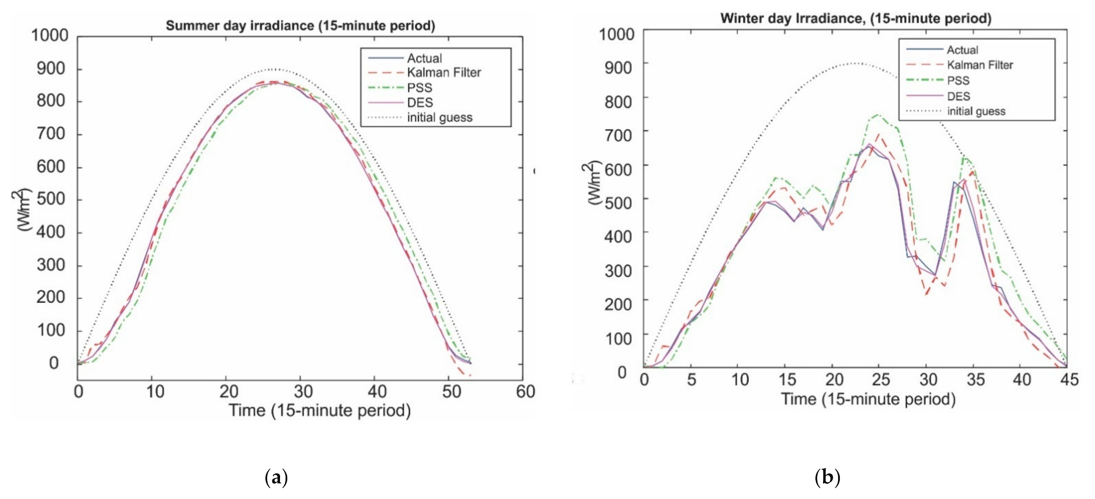
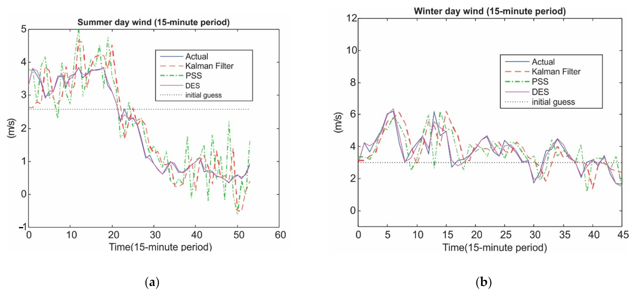
2. Solar Radiation and Wind Speed Forecasting
2.1. Double Exponential Smoothing (DES)
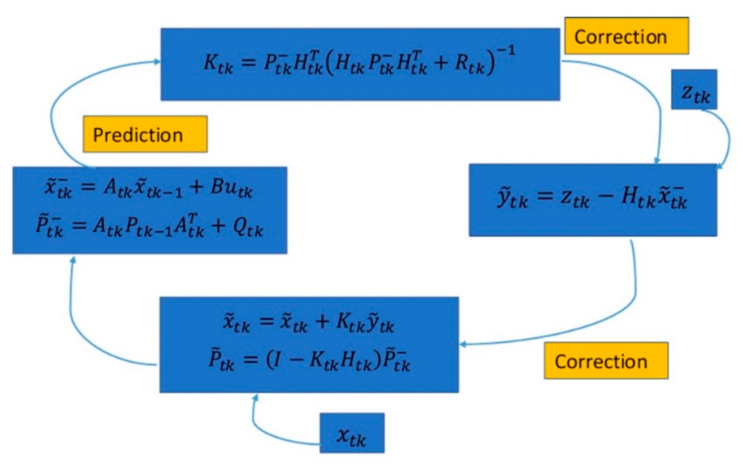
2.2. Kalman Filter
2.3. Persistence Skill Score (PSS)
2.4. Validation Methods
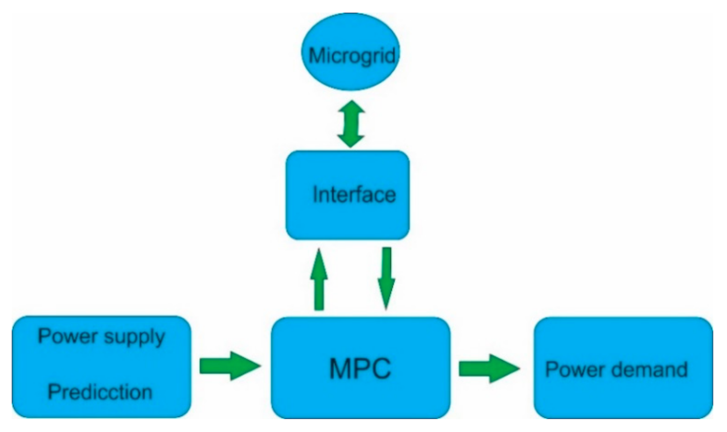
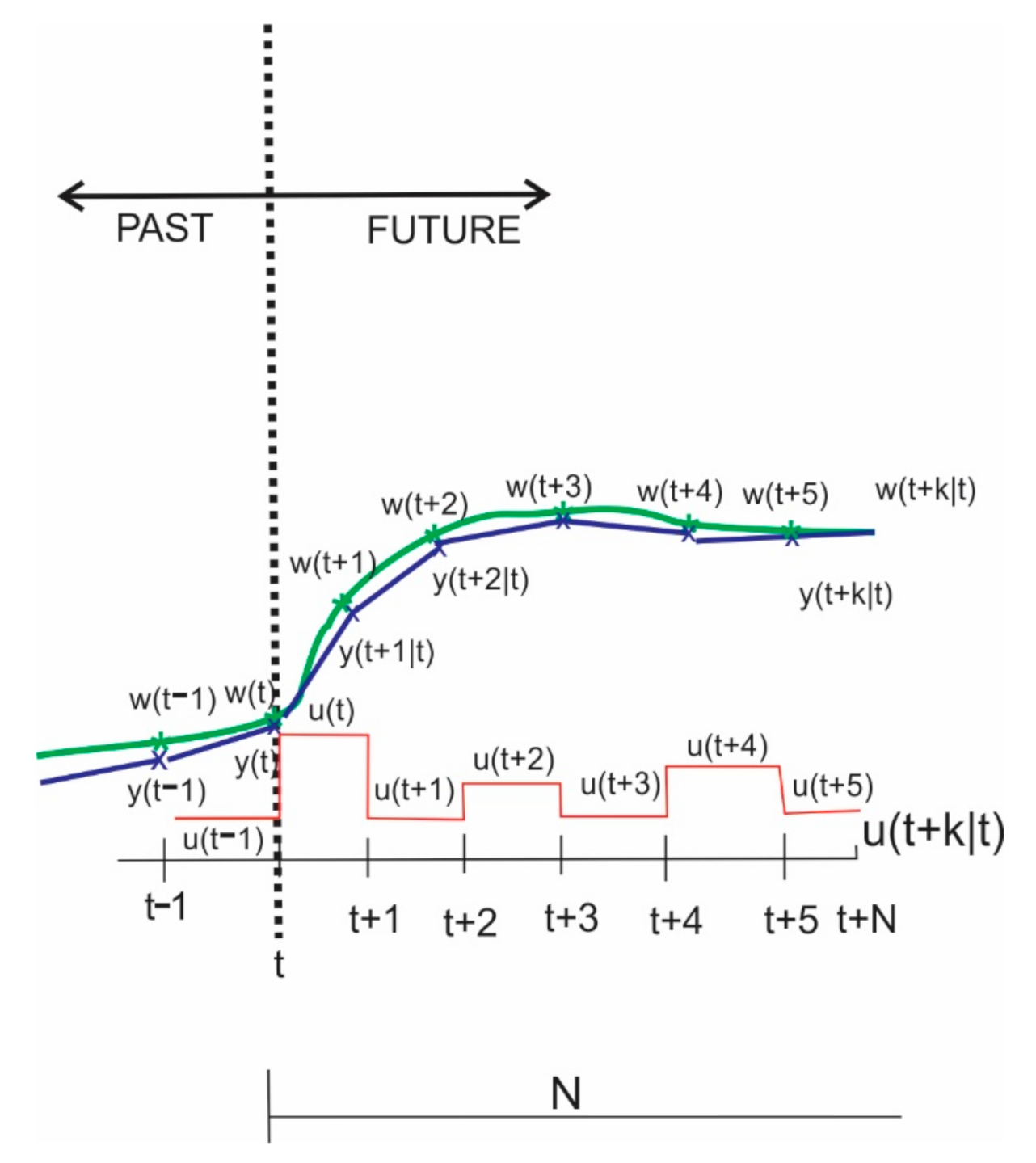
3. Model-Based Predictive Control (MPC)
4. Computational Simulation
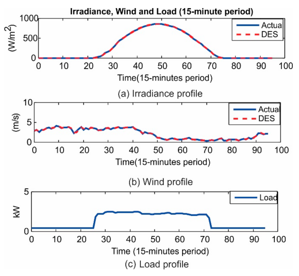
4.1. Simulation Framework
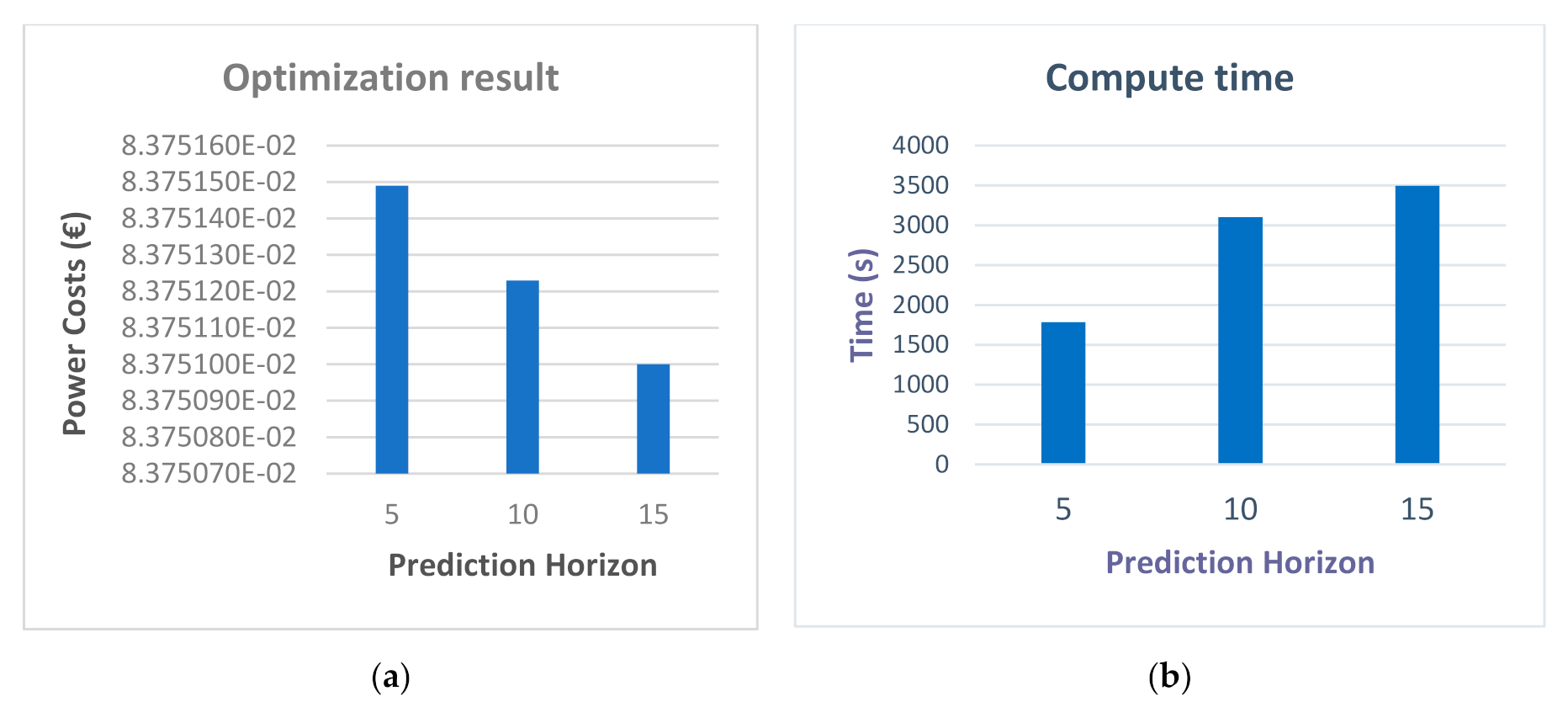
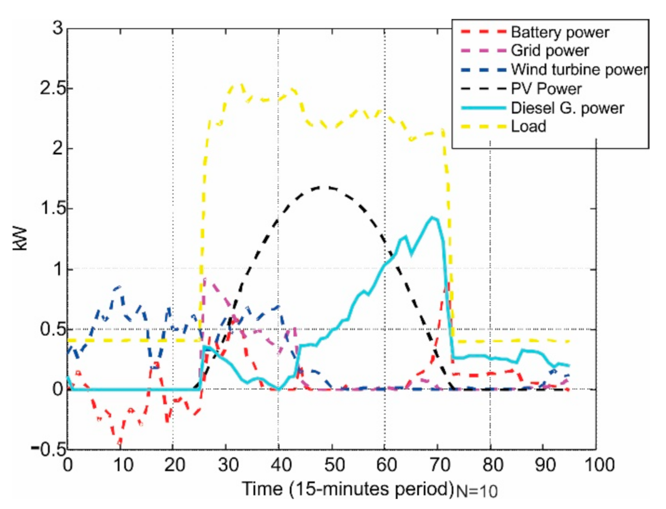
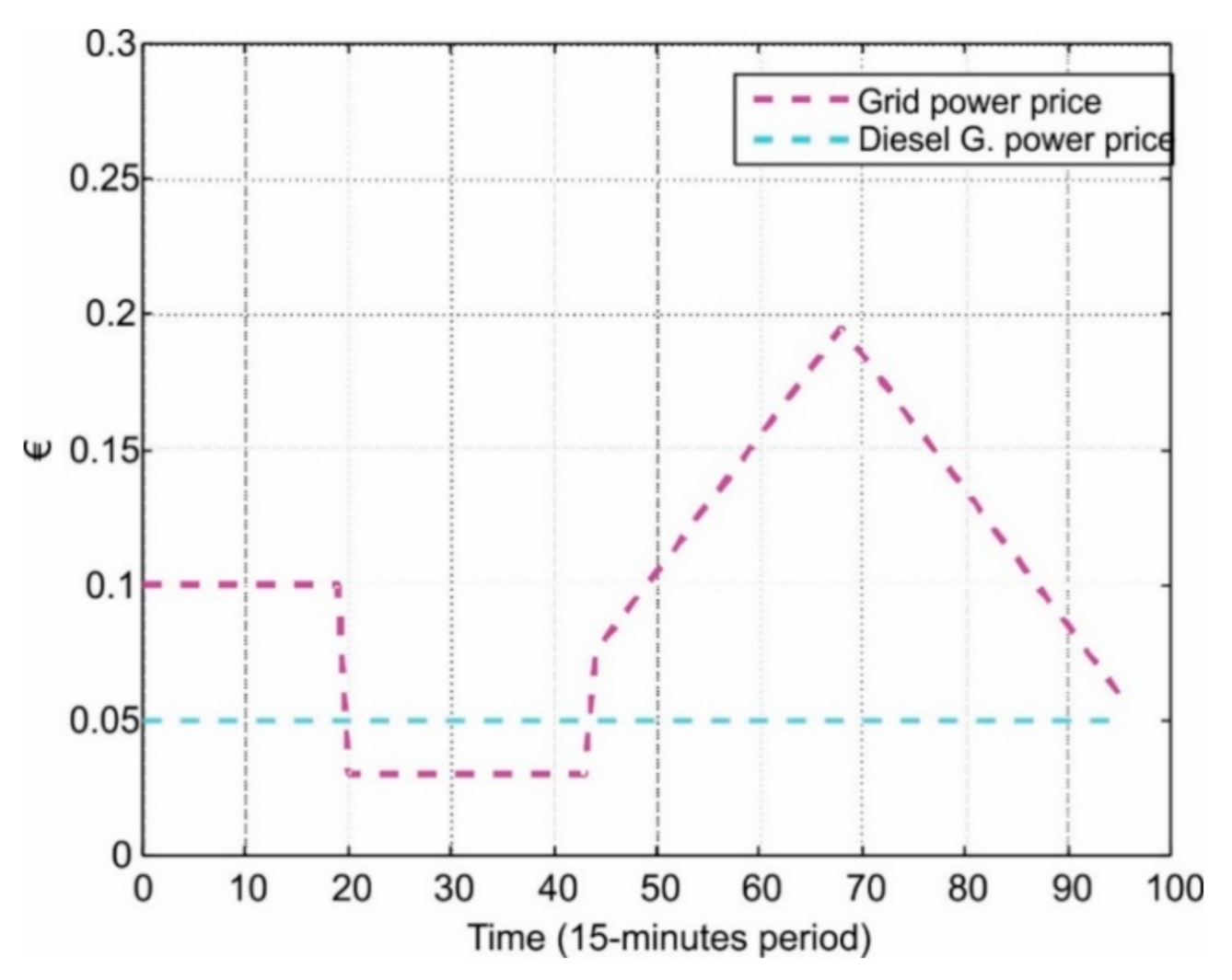
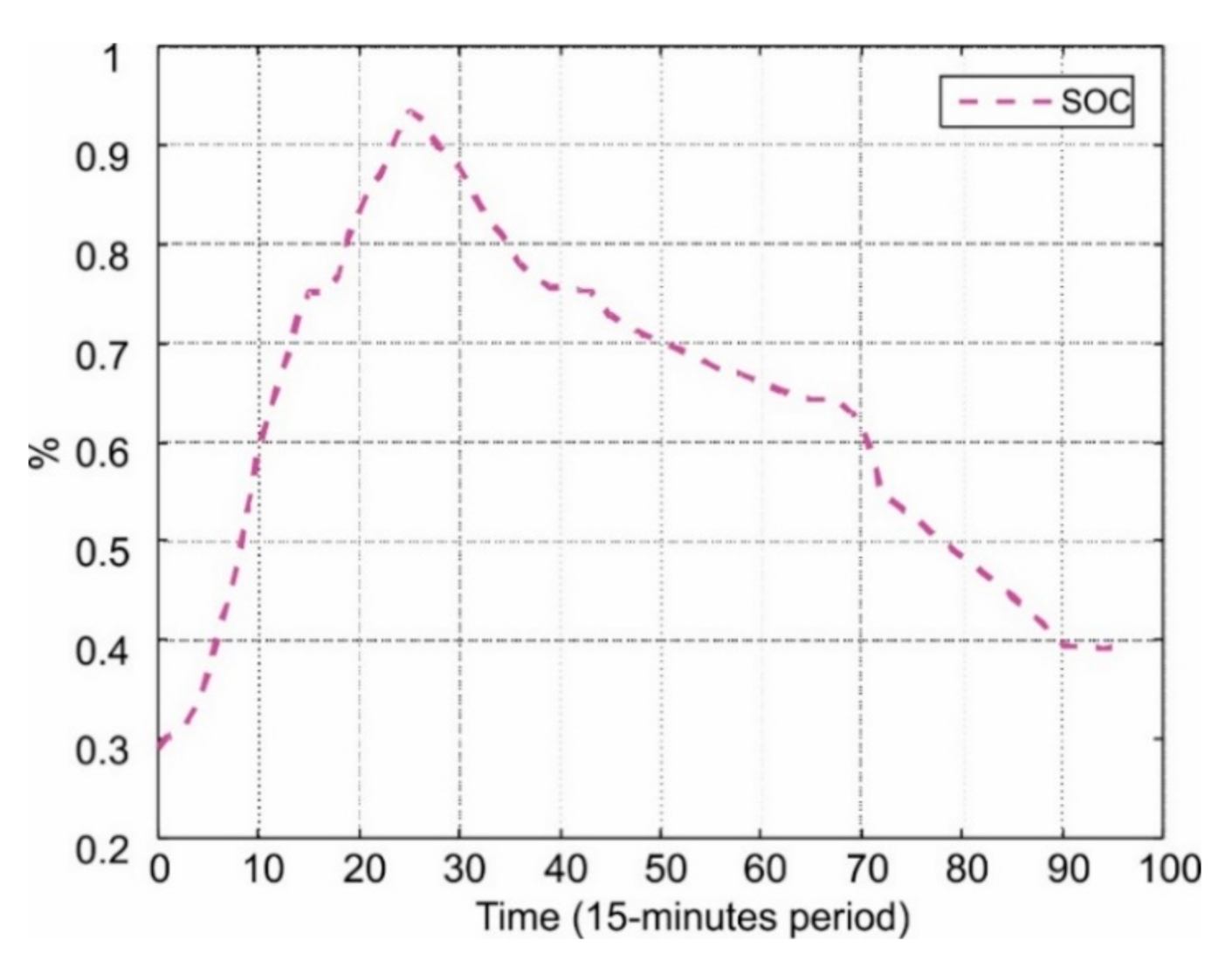
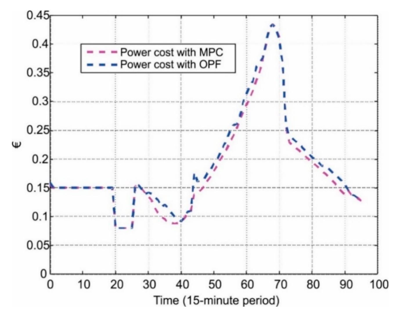
4.2. Results and Discussion
5. Conclusions
Author Contributions
Funding
Institutional Review Board Statement
Informed Consent Statement
Data Availability Statement
Acknowledgments
Conflicts of Interest
Nomenclature
| Objective function | |
| Equality constrains. | |
| Current at PV system terminals | |
| Battery charge power | |
| Battery discharge power | |
| Photovoltaic system power | |
| Panel terminal power | |
| Power at PV system terminals | |
| Active power injected of the microgrid | |
| Active Power of the load | |
| Load power | |
| Main grid power | |
| Wind turbine power | |
| Reactive power injected of the microgrid | |
| Reactive power main grid | |
| Reactive power of the load | |
| Initial state of charge | |
| State of charge | |
| T | Time stages set |
| Time stage | |
| Voltage at PV system terminals | |
| Variable Inequalities constraints | |
| Inequalities constraints |
Appendix A

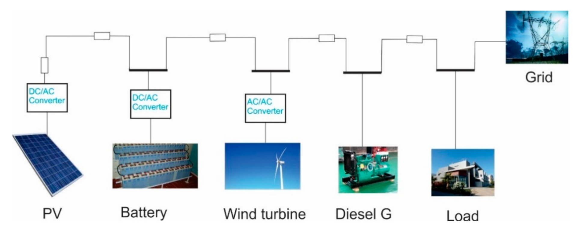
| Battery | Loads | PV | Wind Turbine | G. Disel | |
|---|---|---|---|---|---|
| Unit | 1 | 1 | 1 | 1 | 1 |
| kW | 1 | 3 | 2 | 1 | 2 |
| Volts | 230 ± 5% | 230 ± 5% | 230 ± 5% | 230 ± 5% | 230 ± 5% |
References
- Lee, J.; Zhang, P.; Gan, L.K.; Howey, D.A.; Osborne, M.A.; Tosi, A.; Duncan, S. Optimal Operation of an Energy Management System Using Model Predictive Control and Gaussian Process Time-Series Modeling. IEEE J. Emerg. Sel. Top. Power Electron. 2018, 6, 1783–1795. [Google Scholar] [CrossRef]
- Dkhili, N.; Eynard, J.; Thil, S.; Grieu, S. A survey of modelling and smart management tools for power grids with prolific distributed generation. Sustain. Energy Grids Netw. 2020, 21, 100284. [Google Scholar] [CrossRef]
- Fichera, A.; Marrasso, E.; Sasso, M.; Volpe, R. Energy, Environmental and Economic Performance of an Urban Community Hybrid Distributed Energy System. Energies 2020, 13, 2545. [Google Scholar] [CrossRef]
- Bordons, C.; García-Torres, F.; Valverde, L. Gestión Óptima de la Energía en Microrredes con Generación Renovable. Rev. Iberoam. Automática Informática Ind. RIAI 2015, 12, 117–132. [Google Scholar] [CrossRef]
- Leonori, S.; Martino, A.; Frattale Mascioli, F.M.; Rizzi, A. Microgrid Energy Management Systems Design by Computational Intelligence Techniques. Appl. Energy 2020, 277, 115524. [Google Scholar] [CrossRef]
- Banković, B.; Filipović, F.; Mitrović, N.; Petronijević, M.; Kostić, V. A Building Block Method for Modeling and Small-Signal Stability Analysis of the Autonomous Microgrid Operation. Energies 2020, 13, 1492. [Google Scholar] [CrossRef]
- Olivares, D.E.; Mehrizi-Sani, A.; Etemadi, A.H.; Canizares, C.A.; Iravani, R.; Kazerani, M.; Hajimiragha, A.H.; Gomis-Bellmunt, O.; Saeedifard, M.; Palma-Behnke, R.; et al. Trends in Microgrid Control. IEEE Trans. Smart Grid 2014, 5, 1905–1919. [Google Scholar] [CrossRef]
- Hooshmand, A.; Poursaeidi, M.H.; Mohammadpour, J.; Malki, H.A.; Grigoriads, K. Stochastic model predictive control method for microgrid management. In Proceedings of the 2012 IEEE PES Innovative Smart Grid Technologies (ISGT), Washington, DC, USA, 16–20 January 2012; pp. 1–7. [Google Scholar]
- Cecilia, A.; Carroquino, J.; Roda, V.; Costa-Castelló, R.; Barreras, F. Optimal Energy Management in a Standalone Microgrid, with Photovoltaic Generation, Short-Term Storage, and Hydrogen Production. Energies 2020, 13, 1454. [Google Scholar] [CrossRef]
- K/bidi, F.; Damour, C.; Grondin, D.; Hilairet, M.; Benne, M. Power Management of a Hybrid Micro-Grid with Photovoltaic Production and Hydrogen Storage. Energies 2021, 14, 1628. [Google Scholar] [CrossRef]
- Morstyn, T.; Hredzak, B.; Agelidis, V.G. Dynamic optimal power flow for DC microgrids with distributed battery energy storage systems. In Proceedings of the 2016 IEEE Energy Conversion Congress and Exposition (ECCE), Milwaukee, WI, USA, 18–22 September 2016; pp. 1–6. [Google Scholar]
- Dini, A.; Pirouzi, S.; Norouzi, M.; Lehtonen, M. Hybrid stochastic/robust scheduling of the grid-connected microgrid based on the linear coordinated power management strategy. Sustain. Energy Grids Netw. 2020, 24, 100400. [Google Scholar] [CrossRef]
- Grüne, L. Approximation Properties of Receding Horizon Optimal Control. Jahresbericht Dtsch. Math. 2016, 118, 3–37. [Google Scholar] [CrossRef]
- Numata, M.; Sugiyama, M.; Mogi, G. Barrier Analysis for the Deployment of Renewable-Based Mini-Grids in Myanmar Using the Analytic Hierarchy Process (AHP). Energies 2020, 13, 1400. [Google Scholar] [CrossRef]
- Incremona, G.P.; Cucuzzella, M.; Magni, L.; Ferrara, A. MPC with Sliding Mode Control for the Energy Management System of Microgrids. IFAC-PapersOnLine 2017, 50, 7397–7402. [Google Scholar] [CrossRef]
- Pawlowski, A.; Guzmán, J.L.; Rodríguez, F.; Berenguel, M.; Sánchez, J. Application of time-series methods to disturbance estimation in predictive control problems. In Proceedings of the 2010 IEEE International Symposium on Industrial Electronics, Bari, Italy, 4–7 July 2010; pp. 409–414. [Google Scholar]
- Reikard, G. Predicting solar radiation at high resolutions: A comparison of time series forecasts. Sol. Energy 2009, 83, 342–349. [Google Scholar] [CrossRef]
- Dev, S.; AlSkaif, T.; Hossari, M.; Godina, R.; Louwen, A.; van Sark, W. Solar Irradiance Forecasting Using Triple Exponential Smoothing. In Proceedings of the 2018 International Conference on Smart Energy Systems and Technologies (SEST), Seville, Spain, 10–12 September 2018; pp. 1–6. [Google Scholar]
- Dong, Z.; Yang, D.; Reindl, T.; Walsh, W.M. Short-term solar irradiance forecasting using exponential smoothing state space model. Energy 2013, 55, 1104–1113. [Google Scholar] [CrossRef]
- Soubdhan, T.; Ndong, J.; Ould-Baba, H.; Do, M.-T. A robust forecasting framework based on the Kalman filtering approach with a twofold parameter tuning procedure: Application to solar and photovoltaic prediction. Sol. Energy 2016, 131, 246–259. [Google Scholar] [CrossRef]
- Zheng, Z.; Chen, H.; Luo, X. A Kalman filter-based bottom-up approach for household short-term load forecast. Appl. Energy 2019, 250, 882–894. [Google Scholar] [CrossRef]
- Luan, H. Tran Application of Kalman Filtering for PV Power Prediction in Short-Term Economic Dispatch. Master’s Thesis, College of Engineering and Mineral Resources, West Virginia University, Morgantownm, WV, USA, 2017. [Google Scholar]
- Mayer, M.J.; Gróf, G. Extensive comparison of physical models for photovoltaic power forecasting. Appl. Energy 2021, 283, 116239. [Google Scholar] [CrossRef]
- Ryan, A.G.; Regnier, C.; Divakaran, P.; Spindler, T.; Mehra, A.; Smith, G.C.; Davidson, F.; Hernandez, F.; Maksymczuk, J.; Liu, Y. GODAE OceanView Class 4 forecast verification framework: Global ocean inter-comparison. J. Oper. Oceanogr. 2015, 8, s98–s111. [Google Scholar] [CrossRef]
- Premalatha, N.; Valan Arasu, A. Prediction of solar radiation for solar systems by using ANN models with different back propagation algorithms. J. Appl. Res. Technol. 2016, 14, 206–214. [Google Scholar] [CrossRef]
- Arias-Rosales, A.; LeDuc, P.R. Modeling the transmittance of anisotropic diffuse radiation towards estimating energy losses in solar panel coverings. Appl. Energy 2020, 268, 114872. [Google Scholar] [CrossRef]
- Vermuyten, E.; Meert, P.; Wolfs, V.; Willems, P. Combining Model Predictive Control with a Reduced Genetic Algorithm for Real-Time Flood Control. J. Water Resour. Plan. Manag. 2018, 144. [Google Scholar] [CrossRef]
- Reynolds, J.; Rezgui, Y.; Kwan, A.; Piriou, S. A zone-level, building energy optimisation combining an artificial neural network, a genetic algorithm, and model predictive control. Energy 2018, 151, 729–739. [Google Scholar] [CrossRef]
- Sarimveis, H.; Bafas, G. Fuzzy model predictive control of non-linear processes using genetic algorithms. Fuzzy Sets Syst. 2003, 139, 59–80. [Google Scholar] [CrossRef]
- Clarke, W.C.; Manzie, C.; Brear, M.J. An economic MPC approach to microgrid control. In Proceedings of the 2016 Australian Control Conference (AuCC), Newcastle, NSW, Australia, 3–4 November 2016; pp. 276–281. [Google Scholar]
- Batiyah, S.; Zohrabi, N.; Abdelwahed, S.; Sharma, R. An MPC-Based Power Management of a PV/Battery System in an Islanded DC Microgrid. In Proceedings of the 2018 IEEE Transportation Electrification Conference and Expo (ITEC), Long Beach, CA, USA, 13–15 June 2018; pp. 231–236. [Google Scholar]
- Romero-Quete, D.; Garcia, J.R. An affine arithmetic-model predictive control approach for optimal economic dispatch of combined heat and power microgrids. Appl. Energy 2019, 242, 1436–1447. [Google Scholar] [CrossRef]
- Camacho, E.F.; Bordons, C. Model Predictive Control, 2nd ed.; Advanced Textbooks in Control and Signal Processing; Michael, J., Grimble, M.A.J., Eds.; Springer: London, UK, 2007; ISBN 978-1-85233-694-3. [Google Scholar]
- Mayne, D.Q.; Rawlings, J.B.; Rao, C.V.; Scokaert, P.O.M. Constrained model predictive control: Stability and optimality. Automatica 2000, 36, 789–814. [Google Scholar] [CrossRef]
- Delfino, F.; Ferro, G.; Minciardi, R.; Robba, M.; Rossi, M.; Rossi, M. Identification and optimal control of an electrical storage system for microgrids with renewables. Sustain. Energy Grids Netw. 2019, 17, 100183. [Google Scholar] [CrossRef]
- Petrollese, M.; Valverde, L.; Cocco, D.; Cau, G.; Guerra, J. Real-time integration of optimal generation scheduling with MPC for the energy management of a renewable hydrogen-based microgrid. Appl. Energy 2016, 166, 96–106. [Google Scholar] [CrossRef]
- e Silva, D.P.; Félix Salles, J.L.; Fardin, J.F.; Rocha Pereira, M.M. Management of an island and grid-connected microgrid using hybrid economic model predictive control with weather data. Appl. Energy 2020, 278, 115581. [Google Scholar] [CrossRef]
- Yassuda Yamashita, D.; Vechiu, I.; Gaubert, J.-P. Two-level hierarchical model predictive control with an optimised cost function for energy management in building microgrids. Appl. Energy 2021, 285, 116420. [Google Scholar] [CrossRef]
- Ahmadi, S.E.; Rezaei, N.; Khayyam, H. Energy management system of networked microgrids through optimal reliability-oriented day-ahead self-healing scheduling. Sustain. Energy Grids Netw. 2020, 23, 100387. [Google Scholar] [CrossRef]
- Nelson, J.R.; Johnson, N.G. Model predictive control of microgrids for real-time ancillary service market participation. Appl. Energy 2020, 269, 114963. [Google Scholar] [CrossRef]
- Polanco Vasquez, L.O.; Carreño Meneses, C.A.; Pizano Martínez, A.; López Redondo, J.; Pérez García, M.; Álvarez Hervás, J.D. Optimal Energy Management within a Microgrid: A Comparative Study. Energies 2018, 11, 2167. [Google Scholar] [CrossRef]
- OMIE. Available online: https://www.omie.es/es/sobre-nosotros (accessed on 22 December 2020).
- Pérez-García, M.; Castilla, M.M.; Álvarez, J.D.; Ruano, A.E.; Pérez-García, M. Characterization of an Energy Consumption Model for a Net Zero Energy Building Laboratory. In Proceedings of the EuroSun2016, Palma de Mallorca, Spain, 11–14 October 2016; International Solar Energy Society: Freiburg, Germany, 2016; pp. 1–11. [Google Scholar]


| DES | Kalman Filter | PSS | |||
|---|---|---|---|---|---|
| Solar Irradiation | Summer day | MSE | 3.4866 | 181.7 | 1318.5 |
| RMSE | 1.8673 | 13.479 | 36.311 | ||
| nRMSE | 0.0032877 | 0.023734 | 0.063933 | ||
| Winter day | MSE | 160.68 | 4441.2 | 7408.8 | |
| RMSE | 12.676 | 66.642 | 86.074 | ||
| nRMSE | 0.033513 | 0.17619 | 0.22756 | ||
| Wind | Summer day | MSE | 0.0036451 | 0.38061 | 0.48657 |
| RMSE | 0.060375 | 0.61694 | 0.69755 | ||
| nRMSE | 0.025121 | 0.25669 | 0.29023 | ||
| Winter day | MSE | 0.055068 | 1.034 | 1.2691 | |
| RMSE | 0.23467 | 1.0168 | 1.1265 | ||
| nRMSE | 0.061423 | 0.26615 | 0.29487 |
Publisher’s Note: MDPI stays neutral with regard to jurisdictional claims in published maps and institutional affiliations. |
© 2021 by the authors. Licensee MDPI, Basel, Switzerland. This article is an open access article distributed under the terms and conditions of the Creative Commons Attribution (CC BY) license (https://creativecommons.org/licenses/by/4.0/).
Share and Cite
Vásquez, L.O.P.; Ramírez, V.M.; Langarica Córdova, D.; Redondo, J.L.; Álvarez, J.D.; Torres-Moreno, J.L. Optimal Management of a Microgrid with Radiation and Wind-Speed Forecasting: A Case Study Applied to a Bioclimatic Building. Energies 2021, 14, 2398. https://doi.org/10.3390/en14092398
Vásquez LOP, Ramírez VM, Langarica Córdova D, Redondo JL, Álvarez JD, Torres-Moreno JL. Optimal Management of a Microgrid with Radiation and Wind-Speed Forecasting: A Case Study Applied to a Bioclimatic Building. Energies. 2021; 14(9):2398. https://doi.org/10.3390/en14092398
Chicago/Turabian StyleVásquez, Luis O. Polanco, Víctor M. Ramírez, Diego Langarica Córdova, Juana López Redondo, José Domingo Álvarez, and José Luis Torres-Moreno. 2021. "Optimal Management of a Microgrid with Radiation and Wind-Speed Forecasting: A Case Study Applied to a Bioclimatic Building" Energies 14, no. 9: 2398. https://doi.org/10.3390/en14092398
APA StyleVásquez, L. O. P., Ramírez, V. M., Langarica Córdova, D., Redondo, J. L., Álvarez, J. D., & Torres-Moreno, J. L. (2021). Optimal Management of a Microgrid with Radiation and Wind-Speed Forecasting: A Case Study Applied to a Bioclimatic Building. Energies, 14(9), 2398. https://doi.org/10.3390/en14092398