Abstract
This work proposes an automated reconfiguration system to manage two types of faults in any position inside the solar arrays. The faults studied are the short-circuit to ground and the open wires in the string. These faults were selected because they severely affect power production. By identifying the affected panels and isolating the faulty one, it is possible to recover part of the power loss. Among other types of faults that the system can detect and locate are: diode short-circuit, internal open-circuit, and the degradation of the internal parasitic serial resistance. The reconfiguration system can detect, locate the above faults, and switch the distributed commutators to recover most of the power loss. Moreover, the system can return automatically to the previous state when the fault has been repaired. A SIMULINK model has been built to prove this automatic system, and a simulated numerical experiment has been executed to test the system response to the faults mentioned. The results show that the recovery of power is more than 90%, and the diagnosis accuracy and sensitivity are both 100% for this numerical experiment.
1. Introduction
Several investigations about dynamic reconfiguration systems (DRSs) in photovoltaic (PV) arrays focus on reducing the electrical incompatibilities or mismatches among the solar panels. Studies such as [1,2,3] aim to compensate the losses in the delivered power by the solar installation as fast as possible when mismatching or partial shading occurs. Typically, these mismatches are caused by nonuniform irradiation over the solar array due to temporal events, such as partial shadows over the modules, and other reasons as stated in [4,5].
The cost of adding a dynamic reconfiguration system can negatively affect the return of investment of the PV plant if the power gain obtained with the DRS is not large enough. As mentioned in [6], the aforementioned situation is most probable in the cases in which the DRSs focus solely on solving irradiance mismatches. Nevertheless, a reconfiguration system can be easily justified if it addresses and solves severe faults that affects the PV plant production and/or can generate a security risk [7].
A DRS that mitigates severe faults in a PV installation requires a fault detection subsystem. In this regards, several authors have developed fault detection methods, e.g., [8,9,10,11,12,13,14]. Fault detection methods may use images such as the ones taken by unmanned aerial systems (UASs) that have been proved useful for large PV plants given that the visual data about the site can be taken in relatively short time and does not require additional measurement circuitry [15,16]. Nevertheless, image-based fault detection techniques are not suitable for real-time reconfiguration given that it requires a complex data communication network with a relatively large bandwidth. Fault detection techniques based on measurement of electrical variables such as [17,18] are most suitable for a mitigating faults with DRS.
In this work, we propose a system that reconfigures the PV generators to minimize the power losses when a short-circuit to the ground or a wire open-circuit fault occurs in series-parallel photovoltaic arrays. These two faults cause the disconnection of the entire PV string generating an significant decrease of the yield plant. Other faults such as diode short-circuit, internal open-circuit inside PV modules, and parasitic serial resistance degradation are only located and classified because the power losses caused by each one of these three faults are minimal, affecting mainly the faulty panel.
A similar approach to this paper can be found in [7] where the DRS is proved in a total cross-tied PV array to reconfigure the array when electrical faults happen. Nevertheless, there are substantial differences between our work and others. Our contribution focuses on the following aspects:
- The presented switch matrix is built in a modular and distributed way as close as possible to the PV panel. This approach is opposite to the centralize switching matrix presented in the literature, e.g., [7,19].
- Our work focuses on detecting, locating, and isolating the electrical faults in the PV array. Almost all the DRSs are oriented to reduce mismatching or partial shading problems, except for [7]. When our system isolates the faulty panel, is easy to observe the increment of output power.
- Our systems reconfigure the PV array in simulation time when a critical electrical fault occurs, and when the electrical faults are repaired. This means that the Diagnosis Algorithm has to detect the faults, the position, and classify them, also when the fault is fixed. Then a second algorithm made the reconfiguration of the faulty panel or repaired panel. Our reconfiguration solution is based on a multiple finite state machine and is far different from other solutions reported in the literature as is shown later, because it receives the diagnosis information to take a control action.
- Our diagnostic algorithm is computationally lightweight when compared to other approaches from artificial intelligence, such as neural networks or metaheuristic solutions.
- Our simulated PV array has panel string with commercial size reaching voltages close to 600 volts; this shows the applicability of the solution for actual commercial installations.
- Our numerical experiment is quite different because we simulate an operative point of the PV array, and then we apply 19 fault events in simulation time, one at a time, to see the behavior of the produced power. This way, we prove our solution is more realistic to study current–voltage () curves characteristics.
Automated Fault Management System Approach
The traditional dynamic reconfiguration systems can be transformed into an automated fault management system when capabilities are added to detect and diagnose faults inside the array. This concept is presented in Figure 1, where the block diagram has three main subsystems: the data acquisition system, the control unit, and the switching matrix. In the context of reconfigurable solar arrays, each part has its particular complexity.
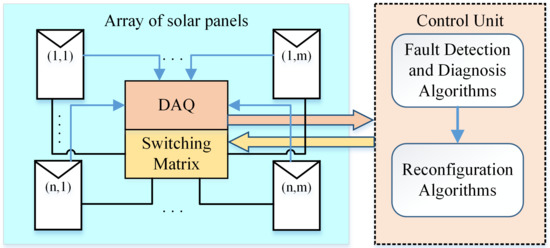
Figure 1.
Block diagram for the automated fault management system.
The data acquisition system (DAQ) captures signals such as currents, voltages, irradiances, and temperatures to estimate the array’s performance. The proposed reconfiguration system’s approach acquires each panel’s differential voltage, the string currents, and the array’s operative voltage. The differential voltage could be measured by simple methods as is proposed in [20,21].
The control unit is responsible for finding whether the solar array has an abnormal issue and for controlling the switches. These tasks are achieved with the following submodules:
- The first submodule aims to determine the condition and fault severity of each panel within the array. In order to do this, signal processing and mathematical modeling techniques are used. An overview of the online, offline techniques for fault detection in solar panels is presented in [22]. Another approach is given by Mellit in [23], where detection and classification techniques are divided in (1) image analysis and (2) electrical characterization. Imaging methods are currently expensive and time consuming, whereas electrical characterization is cheaper and more flexible [24]. The latter methods also can be further split into several branches: signal processing and statistical methods (e.g., [8,25,26]), curve characteristics analysis (e.g., [27,28]), power losses analysis or efficiency analysis (e.g., [17,29,30]), current and/or voltage measurements (e.g., [31,32]), and artificial intelligent methods (e.g., [9,33,34]). The diagnosis algorithm implemented in this work is based on the IF-THEN rules presented by the authors in [35] and follows the diagnosis branch based on current–voltage measurements.
- Once the fault has been determined and located, a second algorithm establishes the configuration that produces an improvement of the output power for the given conditions. In this regard, there are plenty of proposals trying to maximize the output power in the array. For instance, there are approaches based on electric measurements using sorting algorithms [4,36], or based on the equalization of the irradiance [37]. Moreover, there are more elaborated solutions using branches of artificial intelligence, such as algorithms based on metaheuristics techniques [38,39,40,41], algorithms based on diffuse logic [42], procedures based on neural networks [43], algorithms based on rough set [44], or based on the study of the inflection points of the curve I-V [45]. This work uses a simple approach based on a multiple finite state machine that has not been reported in previous articles.
Finally, the switching matrix performs the electrical re-connection according to the results of the reconfiguration algorithm. This matrix is usually implemented with relays, and according to [1] the selected topology defines the complexity of the switching matrix. The proposed reconfiguration system focuses on series-parallel (SP) topologies, however this is not the only array topology but is indeed the most used from the commercial viewpoint [46].
In summary, this article proposes an automated fault management (AFM) system capable of dealing with electrical faults in the solar array. The primary objective is recovering part of the energy loss caused by severe faults. Hence, the modeling process for the photovoltaic generators, fault types description, the switching matrix logic, and the diagnosis/reconfiguration algorithms are presented in Section 2. The planned numerical experiment is shown in Section 2.5, while the results and analysis are given in Section 3. The primary conclusions of this study are pointed out in the last section.
2. Materials and Methods
2.1. Modeling the PV Array
The electrical behavior of the crystalline-silicon solar modules is modeled with the single-diode model (SDM) presented in [47], and according to [48] the errors generated by this model are equivalent to errors produced by the double-diode model at standard test conditions. Specifically, we are using SDM because we are not working under low irradiance conditions in which the carrier-recombination losses in the depletion region are important to consider. Therefore, SDM is accurate enough and is as follows,
where is the photo-generated current, I and V are the current and voltage of the module, and are the parasitic series and parallel resistance, is the dark current saturation of the diode, is the number of cells in series that are in the module, and is the thermal voltage. The is equal to , where k is the Boltzman constant approximately , and q is the electronic charge equal to . Finally, T is the module temperature expressed in Kelvin. Inside Equation (1), the saturation current is affected by the semiconductor material used and by the fabrication process; in order to model this, an ideality constant is introduced. The bypass diode is also presented in the model as , and represent the forward current, the saturation current, and the thermal voltage of the bypass diode, respectively.
The parameter translation models in the function of the irradiance G and temperature T are taken from [49], i.e.,
where is the photo-generated current at standard test conditions (STC), is the irradiance at 1000 W/m, is the module temperature at 298.15 K, is the open-circuit voltage at STC, is the thermal coefficient for open-circuit voltage, and is the thermal coefficient for short-circuit current. The above equations were implemented in SIMULINK ® using the SimPowerSystems Specialized Technology library following the model presented in [18].
The series-parallel PV array is built by three strings of 16 solar modules; each one of the solar modules is identical to that presented in Figure 2, and all of them are fed with identical ambient stimuli, which are irradiance and module temperature at standard test conditions. In addition, a controlled voltage source is used to select the voltage operation point of the array. The voltage is chosen according to the constant voltage method [50] to define the maximum power point as,
where m is the number of modules in the string and and its typical value is given by . Here, the term is the maximum power point voltage of the module reported in the data-sheet.
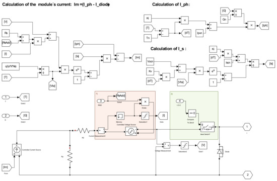
Figure 2.
Model of the photovoltaic module implemented in Simulink.
We use the mathematical matrix notation for locating modules and measurements in the solar array. This means that the physical location or the electrical measurements could be treated with the matrix form. In a PV array which has a size of panels and n strings, the logic position p of each module could be easily defined using an ordered pair of variables such as for elements in the string, and for strings in the array. In this way, the location is defined by ; for instance in the Figure 3, the measured voltage at panel 19 could be expressed as .
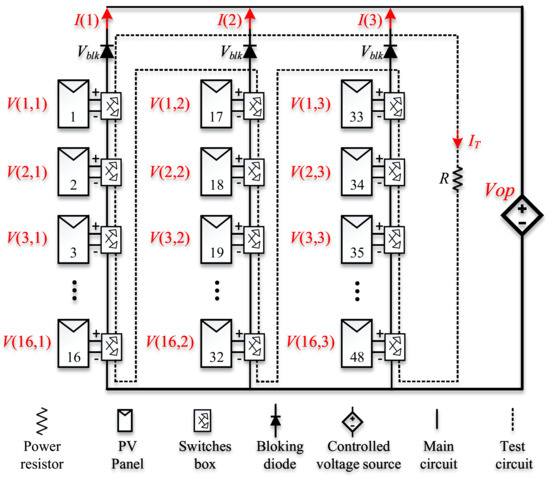
Figure 3.
Photovoltaic array schematic. The electrical measurements are indicated in red color, and the distributed switch boxes for fault reconfiguration are next to the PV panels.
2.2. Modeling the Electrical Faults
The diagnosis and reconfiguration algorithms focus mainly on two faults types that severely affect the power production: the string open-circuit and short-circuit to ground. The string open-circuit occurs when the string fuses burn-out or when module connectors lost conductivity between the PV module and the switching boxes. This fault type is simulated with a controllable normally-close (NC) single-pole single-throw (SPST) switch. On the other hand, the short-circuit to ground occurs when the solar module’s insulation materials, wires, or connectors allow an electrical path to the grounded holding structure. This fault type is simulated with a controllable normally-open (NO) SPST switch that connects the PV module’s positive terminal to the ground.
Assuming that all the modules in a PV array are working close to the maximum power point (MPP), these two faults could generate power losses of around each one per fault. Hence, if simultaneous faults occur in different strings, the power losses should be multiplied by the number of parallel events. This is the reason why we focus on these two faults.
Additionally, other electrical faults such as internal degradation of the PV module, open-circuit inside the PV module, and module’s short-circuit are considered in this study. These faults have less impact on the output power; however, they are no less important because they could conflict with the diagnosis or reconfiguration algorithms. A brief description of each of them is given next:
- Internal degradation: the PV module degradation causes an increase in the internal series resistance [28]. This effect is modeled using a controlled voltage source in series with the PV module internal resistance as shown in the light orange box of Figure 2. The additional resistance value can be modified during the simulation using port three, called RND, shown in Figure 2, when this fault is applied to a specific PV module, the series resistance increases to twice its average value.
- Module’s short circuit: This condition is emulated similarly to the open-circuit fault. A controllable NO SPST switch is included at the PV module’s output parallel with the bypass diode.
Again, assuming that all PV modules are working at MPP, if just one panel presents one of the above three faults, the general power loss could be approximated for severe cases to .
2.3. Modeling the Switching Matrix
The switching matrix was designed to work in a modular and distributed way based on the work of Storey in [51]. As shown in Figure 3, the switching boxes commutate the PV modules between the principal circuit and the alternative test circuit. However, the design can be easily expanded to more strings, as is presented later. In Figure 4, the sub-figures (a), (b) show the single-pole double-throw (SPDT) relay connection to construct a circuit that allows reconnection between two different electrical paths, while (c), (d) show how to connect the panel in short-circuit or open-circuit.
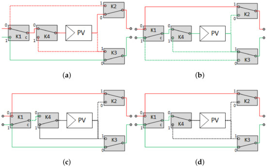
Figure 4.
Safe states for the switching box. (a) State A, panel in the main circuit; (b) State B, panel in the testing circuit; (c) State C, short-circuited panel; (d) State D, panel with open connection.
In the sub-figures, the continuous lines represent electrical connections, and dotted lines represent opening wires. The red color represents the primary circuit, while the green color the alternative circuit. The control signals for the relays are shown in Table 1, where the symbols {1,0,x} represent the logic signals of HIGH, LOW, and “HIGH OR LOW”, respectively.

Table 1.
Control vector for reachable safe states.
The above switching design can be scaled to larger PV systems; for example, the Figure 5 shows the proposed schematic for a array. The designed switching schematic allows not only working with the testing circuit but also allows the PV panel to move among strings. The number of required SPST switches is given by (5), where n represents the number of strings, is the number of panels in the array, and m is the amount of the panels in each string.
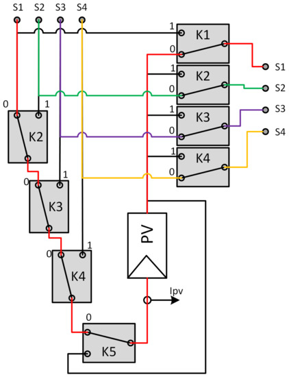
Figure 5.
Modular design of the switching box.
2.4. Modeling the Control Unit
2.4.1. Diagnosis Algorithm
The diagnosis algorithm is based on the logic rules published in [35]. The algorithm requires the following input variables to work; one of them is a matrix voltage V where each cell contains the differential voltage of a module in the PV array. In addition, a vector I where each cell contains the string’s current. Other inputs are the array’s operative voltage , the open-circuit voltage of one reference module , and the current of one particular circuit made to test faulty modules.
The algorithm outputs a matrix O of size where each cell is filled with a number indicating a specific characteristic as shown in Table 2. The algorithm also requires four values: the acceptance level of power loss , a voltage threshold , the blocking diode voltage , and the quantization interval introduced by the analog to digital converter. The diagnosis algorithm based on IF-THEN rules is presented in Algorithm 1.
Table 2.
Tags for fault classification.
2.4.2. Reconfiguration Algorithm
For this work, the reconfiguration algorithm is based on a multiple finite state machine, which means that many identical state machines are running simultaneously. In this way, each switch box has its finite state machine that controls the relay combinations. We only use two combinations of relays for this job: States A and B in Figure 4. The other states are used for testing or isolation procedures not shown here to reduce the complexity.
| Algorithm 1: Diagnosis algorithm based on electrical characterization |
 |
A multiple finite state machine is formed by several identical state machines running in parallel, as shown in the Figure 6. Each state machine controls a specific switch box in the figure. Furthermore, the assignation is represented with the sub-index number in the transition-conditions and states. As it was mentioned before, every state machine has two states and two transitions; the logic for the kth switch box, which is located in the position of the array, is described next:
- At the beginning, the kth PV module is connected to the main circuit, which means that it is in state .
- If the kth PV panel has an open wire, or if the module is the first one with a short-circuit to the ground, the panel will be moved to the testing circuit (State ). The transition-condition expressed as in Equation (6) changes between the two states.
- Now the faulty panel is in state connected in the testing circuit, but if it is repaired, the AFM system will identify the PV module’s working conditions. Hence, the kth PV panel is returned to the main circuit, and this is done with transition-condition as in Equation (7).
In the transition equations, the variable contains the result of the diagnosis algorithm for the module position .

Figure 6.
Multiple finite sate machine which describes the control of the distributed switch boxes.
2.5. Numerical Experiments
To prove the AFM system, a numerical experiment was implemented and executed over Matlab 2015a, running Simulink version 8.5, and the toolbox SimPowerSystems Specialized Technology 2015. The simulated experiment has all the subsystems presented in Figure 1 which are: the PV array of modules, analog to digital converters, the distributed switching boxes, and the control unit, which is composed of the diagnosis algorithm and the reconfiguration algorithm. The PV array has been sized in such a way that it is compatible with the most common commercially available grid-tied inverters, e.g., a 600 V 6 kW inverter.
The PV array operates under the non-fault condition in an operating point close to the maximum power, specifically at a voltage of . During the experiment time, several fault events are applied to the PV array to look at the power behavior and analyze the algorithm results.
Every module is characterized by the well-known model of five parameters presented in Section 2.1, and its parameters are taken from [49] and shown in Table 3 and Table 4. The cell temperature is considered constant in all the modules (K) as well as the global irradiance of (1000 W/m). Furthermore, the electrical cables were modeled as AWG # 10 with a resistance of 3.27 /Km, and assuming a photovoltaic string length of 30 m. The resistance in the testing circuit was calculated as . Regarding the DAQ implementation, a zero order hold was programmed with a sampling time of 0.1 s, and the quantizer discretizes the signals in 0.05 intervals.
Table 3.
Values of the five-parameter model of the KC200GR [49].
Table 4.
Electrical performance at standard test conditions (STC).
Additionally, each of the 19 simulated events has a duration of 0.5 s and the entire experiment lasts 22 s. It is clear that radiation changes across the day, however in tropical countries, with sunshine skies, we could consider the temperature and irradiance constants for a small-time span of less than 36 s in the range hours of , and according to [18] the irradiance variations, for a specific day and location are around for that time span.
The proposed experiment is presented in the Table 5; the second column describes the fault types, and the third column, the duration of the event. The fourth column indicates the PV numeric label, and the fifth column indicates the expected result of the diagnosis algorithm when it works in an open-loop. Here, open-loop means without feeding the reconfiguration algorithm. Figure 7 shows the fault locations in the array, and the Figure A1 in the Appendix A shows the implemented test bench.
Table 5.
Programmed events applied to the PV plant and the expected diagnosis results.
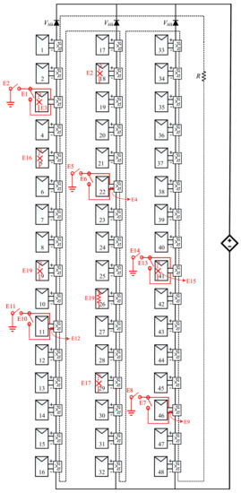
Figure 7.
Location of the fault events inside the PV array.
3. Results
The results of the AFM system are presented graphically. Firstly, the ribbon chart in Figure 8 shows the automatic fault classification made in simulation time (real-time for us) by the diagnosis algorithm. Secondly, Figure 9 shows two power curves; one curve representing the output power behavior when we execute the whole experiment without the AFM system, and the other one when we execute the experiment again but with the AFM system working.
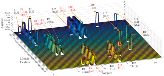
Figure 8.
Plotted results of the diagnosis algorithm.
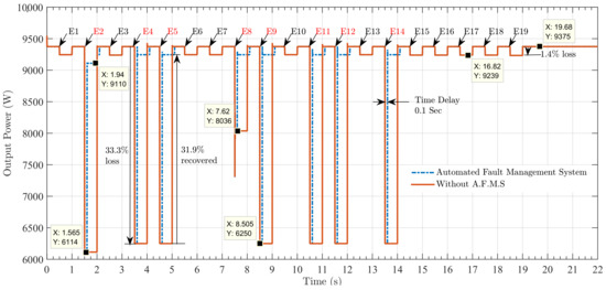
Figure 9.
The behavior of the output power with different electrical faults in the PV array.
The axes in the Figure 8 describe the PV location of the module, the sample time and the fault classification. The results are presented in a ribbon chart where discrete levels of height range from 0 to 7 values according to the Table 2. In the figure, every ribbon represents a PV module, and the working and faultless PV modules are represented with the number zero. For a specific ribbon, if the number is higher than one, it means that a fault condition is occurring in that precise sample time. The fault events are pointed in the figure, and below them, the PV tag and diagnosis result is shown, i.e., . It is easy to observe from the figure that the experiment sequence was correctly decoded as it is presented in (8),
The planned sequence of fault events mixes faults with different severity levels; for instance, the short-circuit to the ground or an open-wire fault causes much more power losses in the PV array than minor faults such as a short-circuiting diode, internal degradation, or internal open-circuit. In this sense, the presented AFM system locates and diagnoses the PV modules with a slight time delay of just one sample.
Additionally, notice in Figure 8 that events {E2, E4, E5, E8, E9, E11, E12, E14} are the ones which affect several modules in one string. This event list is associated only with short-circuit-to-ground faults or open wire in the string. When these two fault types happen, they generate one faulty module and affected modules. For example, the event E4 over module 22 is an open wire between the module and the switching box; the figure shows that PV modules are affected and are classified as modules with open-circuit voltage, and the faulty panel 22 is the one with the defect. Moreover, other events like E11, which is the short-circuit to ground over module 11, generate affected modules. In this case, modules located above module 11 are in open-circuit voltage (this means a tag number less than eleven). In contrast, modules below module 11 are classified as short-circuited to the ground (this means a tag number higher than eleven).
4. Discussion
The AFM system’s results are entirely satisfactory for several reasons, among them: real-time diagnosis without false positives or false negatives, real-time reconfiguration sensible to critical faults, and high recovery of power loss after reconfiguration.
In Figure 8, it is easy to observe that the number of false positive (FP) or false negative (FN) detections are zero. For example, capturing the FP could be understood when there is no AFM system detection while the programmed fault occurs. On the other hand, capturing the FN could be appreciated when detection results appear in time periods without programmed faults. In both cases, the counting of FP and FN indicates that the accuracy and sensitivity are 100% for this experiment. This means that the diagnosis algorithm detects only the positive cases and detects only the negative ones.
As mentioned before, the Figure 9 shows the output power behavior with and without the AFM system. When the AFM system is not working and the fault sequence is applied to the array, the produced power drops depending on the fault type. Minor faults events like module short-circuit, internal open-circuit, or internal degradation, generate small losses around of the total produced power, i.e., less than 2.1%. However, when the fault type is a short-circuit to the ground or an open-wire in one string, the harm in the production power is notorious. For instance, when the events E2, E4, E5, E8, E9, E11, E12, and E14 happen, the power production drops, as it is shown in the third column on Table 6. Although, when the AFM system works properly, the power loss recovery is more than 90% for all the severe cases; therefore, the effect in the total power is minimum, as shown in the fifth column in the Table 6.
Table 6.
Power loss and recovered power with the system.
In addition, a positive aspect of this diagnosis and reconfiguration system is the automatic detection of the recovered panels; this means that the system can return to the original array configuration when the fault is repaired. This can be observed in Figure 9.
An important characteristic of the diagnosis algorithm is the low number of operations required to classify the elements in the PV array. Moreover, the algorithm complexity is , where the logarithmic term comes from the ordering required in line 9 in Algorithm 1. Notice that in other research papers such as [7,32] or specialize reviews such as [8,23], the computational complexity of the solutions are not addressed.
As a future work, the impact of the variability of the PV array irradiances and temperatures in the algorithm will be analyzed. It is of special interest to tune the proposed algorithm in such a way that fast changing irradiances do not produce false positive or false negatives. In addition, the effect of external faults outside the PV array has to considered; for instance, faults in the inverters or power transformer are topics interesting to incorporate for future work.
5. Conclusions
We have presented an automated fault management system composed of three main parts: the diagnosis algorithm, the reconfiguration algorithm, and the distributed switching matrix. The AFM system was tested using a solar array composed of PV modules and 19 events that use 5 electrical faults. The simulated faults have different severity levels, and for the short-circuit to the ground or an open-wire, the AFM system recovers more than 90% of the power loss with a diagnosis accuracy and sensitivity of 100% for the planned experiments.
The diagnosis algorithm is lightweight because it is based on IF-THEN rules derived from circuit analysis theory applied to the PV array. This is a vital aspect against other classification techniques like artificial neural networks, support vector machines, k-nearest neighbor, etc., because our diagnosis method based on behavioral rules processes the data with only a sample delay. No data training is required, which is suitable to be implemented using micro-controllers or IoT devices.
Author Contributions
Conceptualization, C.M. and L.D.M.-S.; methodology, L.D.M.-S.; software, L.D.M.-S.; validation, L.D.M.-S. and C.M.; formal analysis, L.D.M.-S.; investigation, L.D.M.-S. and C.M.; resources C.M.; data curation, L.D.M.-S.; writing—original draft preparation, L.D.M.-S.; writing—review and editing, C.M.; visualization, L.D.M.-S.; supervision, C.M.; project administration, C.M.; funding acquisition, C.M. All authors have read and agreed to the published version of the manuscript.
Funding
This work was supported by scholarship program of the Costa Rica Institute of Technology and the VIE project 5402-1341-1701.
Institutional Review Board Statement
Not applicable.
Informed Consent Statement
Not applicable.
Acknowledgments
Special thanks to all SESLab members for apportioning support and ideas http://www.ie.tec.ac.cr/seslab/pmwiki/pmwiki.php/Main/Team accessed on 16 April 2021.
Conflicts of Interest
The authors declare no conflict of interest.
Abbreviations
The following abbreviations are used in this manuscript:
| MDPI | Multidisciplinary Digital Publishing Institute |
| DOAJ | Directory of open access journals |
| PV | Photo-voltaic |
| SDM | Single-Diode Model |
| STC | Standard Test Conditions |
| DRS | Dynamic Reconfiguration Systems |
| AFM | Automated Fault Management |
| SC | Short Circuit |
| OC | Open Circuit |
| NC | Normally-close |
| NO | Normally-open |
| DAQ | Data acquisition system |
| SPST | Single-Pole Single-Throw |
| SPDT | Single-Pole Double-Throw |
| FP | False Positive |
| FN | False Negative |
Appendix A

Figure A1.
Test bench for the numerical experiment.
References
- La Manna, D.; Li Vigni, V.; Riva Sanseverino, E.; Di Dio, V.; Romano, P. Reconfigurable electrical interconnection strategies for photovoltaic arrays: A review. Renew. Sustain. Energy Rev. 2014, 33, 412–426. [Google Scholar] [CrossRef]
- Spagnuolo, G.; Petrone, G.; Lehman, B.; Ramos Paja, C.A.; Zhao, Y.; Orozco Gutierrez, M.L. Control of photovoltaic arrays: Dynamical reconfiguration for fighting mismatched conditions and meeting load requests. IEEE Ind. Electron. Mag. 2015, 9, 62–76. [Google Scholar] [CrossRef]
- Malathy, S.; Ramaprabha, R. Reconfiguration strategies to extract maximum power from photovoltaic array under partially shaded conditions. Renew. Sustain. Energy Rev. 2018, 81, 2922–2934. [Google Scholar] [CrossRef]
- Parlak, K. PV array reconfiguration method under partial shading conditions. Int. J. Electr. Power Energy Syst. 2014, 63, 713–721. [Google Scholar] [CrossRef]
- Dhimish, M.; Holmes, V.; Mehrdadi, B.; Dales, M.; Chong, B.; Zhang, L. Seven indicators variations for multiple PV array configurations under partial shading and faulty PV conditions. Renew. Energy 2017, 113, 438–460. [Google Scholar] [CrossRef]
- Schettino, G.; Pellitteri, F.; Ala, G.; Miceli, R.; Romano, P.; Viola, F. Dynamic Reconfiguration Systems for PV Plant: Technical and Economic Analysis. Energies 2020, 13, 2004. [Google Scholar] [CrossRef]
- Ji, D.; Zhang, C.; Lv, M.; Ma, Y.; Guan, N. Photovoltaic Array Fault Detection by Automatic Reconfiguration. Energies 2017, 10, 699. [Google Scholar] [CrossRef]
- Garoudja, E.; Harrou, F.; Sun, Y.; Kara, K.; Chouder, A.; Silvestre, S. Statistical fault detection in photovoltaic systems. Sol. Energy 2017, 150, 485–499. [Google Scholar] [CrossRef]
- Liu, G.; Yu, W.; Zhu, L. Condition classification and performance of mismatched photovoltaic arrays via a pre-filtered Elman neural network decision making tool. Sol. Energy 2018, 173, 1011–1024. [Google Scholar] [CrossRef]
- Appiah, A.Y.; Zhang, X.; Ayawli, B.B.K.; Kyeremeh, F. Review and Performance Evaluation of Photovoltaic Array Fault Detection and Diagnosis Techniques. Int. J. Photoenergy 2019, 2019, 1–19. [Google Scholar] [CrossRef]
- Jadidi, S.; Badihi, H.; Zhang, Y. Passive Fault-Tolerant Control Strategies for Power Converter in a Hybrid Microgrid. Energies 2020, 13, 5625. [Google Scholar] [CrossRef]
- Chaudhary, A.S.; Chaturvedi, D. Thermal Image Analysis and Segmentation to Study Temperature Effects of Cement and Bird Deposition on Surface of Solar Panels. Int. J. Image Graph. Signal Process. 2017, 9, 12–22. [Google Scholar] [CrossRef]
- Leva, S.; Aghaei, M.; Grimaccia, F. PV power plant inspection by UAS: Correlation between altitude and detection of defects on PV modules. In Proceedings of the 2015 IEEE 15th International Conference on Environment and Electrical Engineering (EEEIC), Rome, Italy, 10–13 June 2015; IEEE: New York, NY, USA, 2015. [Google Scholar]
- Cardinale-Villalobos, L.; Rimolo-Donadio, R.; Meza, C. Solar Panel Failure Detection by Infrared UAS Digital Photogrammetry: A Case Study. Int. J. Renew. Energy Res. (IJRER) 2020, 10, 1154–1164. [Google Scholar]
- Cardinale-Villalobos, L.; Meza, C.; Murillo-Soto, L. Experimental Comparison of Visual Inspection and Infrared Thermography for the Detection of Soling and Partial Shading in Photovoltaic Arrays. In ICSC-CITIES 2020. Communications in Computer and Information Science; Springer: Cham, Switzerland, 2021; Volume 1359. [Google Scholar]
- Tyutyundzhiev, N.; Lovchinov, K.; Martínez-Moreno, F.; Leloux, J.; Narvarte, L. Advanced PV modules inspection using multirotor UAV. In Proceedings of the 31st European Photovoltaic Solar Energy Conference and Exhibition, Hamburg, Germany, 14–18 September 2015. [Google Scholar]
- Murillo-Soto, L.D.; Meza, C. Fault detection in solar arrays based on an efficiency threshold. In Proceedings of the 2020 IEEE 11th Latin American Symposium on Circuits & Systems (LASCAS), San Jose, Costa Rica, 25–28 February 2020; IEEE: New York, NY, USA, 2020; pp. 1–4. [Google Scholar]
- Murillo-Soto, L.D.; Meza, C. Photovoltaic Array Fault Detection Algorithm Based on Least Significant Difference Test. In Applied Computer Sciences in Engineering; Figueroa-García, J.C., Garay-Rairán, F.S., Hernández-Pérez, G.J., Díaz-Gutierrez, Y., Eds.; Springer International Publishing: Cham, Switzerland, 2020; pp. 501–515. [Google Scholar]
- Serna-Garcés, S.; Bastidas-Rodríguez, J.; Ramos-Paja, C. Reconfiguration of Urban Photovoltaic Arrays Using Commercial Devices. Energies 2016, 9, 2. [Google Scholar] [CrossRef]
- Murillo-Soto, L.D.; Meza, C. Voltage measurement in a reconfigurable solar array with series-parallel topology. In Proceedings of the 2017 IEEE 37th CONCAPAN, Managua, Nicaragua, 15–17 November 2017; IEEE: Managua, Nicaragua, 2017; pp. 1–5. [Google Scholar] [CrossRef]
- Kabalci, Y.; Kabalci, E. The low cost voltage and current measurement device design for power converters. In Proceedings of the 2016 8th International Conference on Electronics, Computers and Artificial Intelligence (ECAI), Ploiesti, Romania, 30 June–2 July 2016; IEEE: New York, NY, USA, 2016; pp. 1–6. [Google Scholar] [CrossRef]
- Bastidas-Rodriguez, J.; Petrone, G.; Ramos-Paja, C.; Spagnuolo, G. Photovoltaic modules diagnostic: An overview. In Proceedings of the IECON 2013—39th Annual Conference of the IEEE Industrial Electronics Society, Vienna, Austria, 10–13 November 2013; IEEE: New York, NY, USA, 2013; pp. 96–101. [Google Scholar] [CrossRef]
- Mellit, A.; Tina, G.; Kalogirou, S. Fault detection and diagnosis methods for photovoltaic systems: A review. Renew. Sustain. Energy Rev. 2018, 91, 1–17. [Google Scholar] [CrossRef]
- Chen, H.; Yi, H.; Jiang, B.; Zhang, K.; Chen, Z. Data-Driven Detection of Hot Spots in Photovoltaic Energy Systems. IEEE Trans. Syst. Man Cybern. Syst. 2019, 49, 1731–1738. [Google Scholar] [CrossRef]
- Zhao, Y.; Lehman, B.; Ball, R.; Mosesian, J.; de Palma, J.F. Outlier detection rules for fault detection in solar photovoltaic arrays. In Proceedings of the 2013 Twenty-Eighth Annual IEEE Applied Power Electronics Conference and Exposition (APEC), Long Beach, CA, USA, 17–21 March 2013; pp. 2913–2920. [Google Scholar] [CrossRef]
- Chen, G.; Lin, P.; Lai, Y.; Chen, Z.; Wu, L.; Cheng, S. Location for fault string of photovoltaic array based on current time series change detection. Energy Procedia 2018, 145, 406–412. [Google Scholar] [CrossRef]
- Chine, W.; Mellit, A.; Pavan, A.M.; Lughi, V. Fault diagnosis in photovoltaic arrays. In Proceedings of the 2015 International Conference on Clean Electrical Power (ICCEP), Taormina, Italy, 16–18 June 2015; IEEE: New York, NY, USA, 2015; pp. 67–72. [Google Scholar] [CrossRef]
- Bastidas-Rodriguez, J.D.; Franco, E.; Petrone, G.; Ramos-Paja, C.A.; Spagnuolo, G. Model-Based Degradation Analysis of Photovoltaic Modules Through Series Resistance Estimation. IEEE Trans. Ind. Electron. 2015, 62, 7256–7265. [Google Scholar] [CrossRef]
- Chouder, A.; Silvestre, S. Automatic supervision and fault detection of PV systems based on power losses analysis. Energy Convers. Manag. 2010, 51, 1929–1937. [Google Scholar] [CrossRef]
- Huang, C.; Wang, L. Simulation study on the degradation process of photovoltaic modules. Energy Convers. Manag. 2018, 165, 236–243. [Google Scholar] [CrossRef]
- Banavar, M.; Braun, H.; Buddha, S.T.; Krishnan, V.; Spanias, A.; Takada, S.; Takehara, T.; Tepedelenlioglu, C.; Yeider, T. Signal processing for solar array monitoring, fault detection, and optimization. Synth. Lect. Power Electron. 2012, 7, 1–95. [Google Scholar] [CrossRef]
- Pei, T.; Zhang, J.; Li, L.; Hao, X. A fault locating method for PV arrays based on improved voltage sensor placement. Sol. Energy 2020, 201, 279–297. [Google Scholar] [CrossRef]
- Chine, W.; Mellit, A.; Lughi, V.; Malek, A.; Sulligoi, G.; Massi Pavan, A. A novel fault diagnosis technique for photovoltaic systems based on artificial neural networks. Renew. Energy 2016, 90, 501–512. [Google Scholar] [CrossRef]
- Dhimish, M.; Holmes, V.; Mehrdadi, B.; Dales, M. Diagnostic method for photovoltaic systems based on six layer detection algorithm. Electr. Power Syst. Res. 2017, 151, 26–39. [Google Scholar] [CrossRef]
- Murillo-Soto, L.D.; Meza, C. Diagnose Algorithm and Fault Characterization for Photovoltaic Arrays: A Simulation Study. In ELECTRIMACS 2019; Zamboni, W., Petrone, G., Eds.; Springer International Publishing: Cham, Switzerland, 2020; pp. 567–582. [Google Scholar]
- Nguyen, D.; Lehman, B. An Adaptive Solar Photovoltaic Array Using Model-Based Reconfiguration Algorithm. IEEE Trans. Ind. Electron. 2008, 55, 2644–2654. [Google Scholar] [CrossRef]
- Velasco-Quesada, G.; Guinjoan-Gispert, F.; Pique-Lopez, R.; Roman-Lumbreras, M.; Conesa-Roca, A. Electrical PV Array Reconfiguration Strategy for Energy Extraction Improvement in Grid-Connected PV Systems. IEEE Trans. Ind. Electron. 2009, 56, 4319–4331. [Google Scholar] [CrossRef]
- Deshkar, S.N.; Dhale, S.B.; Mukherjee, J.S.; Babu, T.S.; Rajasekar, N. Solar PV array reconfiguration under partial shading conditions for maximum power extraction using genetic algorithm. Renew. Sustain. Energy Rev. 2015, 43, 102–110. [Google Scholar] [CrossRef]
- Camarillo-Peñaranda, J.R.; Ramírez-Quiroz, F.A.; González-Montoya, D.; Bolaños-Martínez, F.; Ramos-Paja, C.A. Reconfiguration of photovoltaic arrays based on genetic algorithm. Rev. Fac. Ing. Univ. Antioq. 2015, 75, 95–107. [Google Scholar] [CrossRef]
- Carotenuto, P.; Della Cioppa, A.; Marcelli, A.; Spagnuolo, G. An evolutionary approach to the dynamical reconfiguration of photovoltaic fields. Neurocomputing 2015, 170, 393–405. [Google Scholar] [CrossRef]
- Balato, M.; Costanzo, L.; Vitelli, M. Reconfiguration of PV modules: A tool to get the best compromise between maximization of the extracted power and minimization of localized heating phenomena. Sol. Energy 2016, 138, 105–118. [Google Scholar] [CrossRef]
- Karakose, M.; Baygin, M.; Baygin, N.; Murat, K.; Akin, E. An intelligent reconfiguration approach based on fuzzy partitioning in PV arrays. In Proceedings of the INISTA 2014—IEEE International Symposium on Innovations in Intelligent Systems and Applications, Proceedings, Alberobello, Italy, 23–25 June 2014; pp. 356–360. [Google Scholar] [CrossRef]
- Karakose, M.; Baygin, M.; Parlak, K.S. A new real-time reconfiguration approach based on neural network in partial shading for PV arrays. In Proceedings of the 2014 International Conference on Renewable Energy Research and Application (ICRERA), Milwaukee, WI, USA, 19–22 October 2014; IEEE: New York, NY, USA, 2014; pp. 633–637. [Google Scholar] [CrossRef]
- Dos Santos Vicente, P.; Pimenta, T.C.; Ribeiro, E.R. Photovoltaic Array Reconfiguration Strategy for Maximization of Energy Production. Int. J. Photoenergy 2015, 2015, 1–11. [Google Scholar] [CrossRef]
- Orozco-Gutierrez, M.L.; Spagnuolo, G.; Ramirez-Scarpetta, J.M.; Petrone, G.; Ramos-Paja, C.A. Optimized Configuration of Mismatched Photovoltaic Arrays. IEEE J. Photovolt. 2016, 6, 1210–1220. [Google Scholar] [CrossRef]
- Belhaouas, N.; Ait Cheikh, M.-S.; Agathoklis, P.; Oularbi, M.R.; Amrouche, B.; Sedraoui, K.; Djilali, N. PV array power output maximization under partial shading using new shifted PV array arrangements. Appl. Energy 2017, 187, 326–337. [Google Scholar] [CrossRef]
- Petrone, G.; Ramos-Paja, C.A.; Spagnuolo, G.; Xiao, W. Photovoltaic Sources Modeling; Wiley Online Library: Hoboken, NJ, USA, 2017. [Google Scholar]
- Shannan, N.M.A.A.; Yahaya, N.Z.; Singh, B. Single-diode model and two-diode model of PV modules: A comparison. In Proceedings of the 2013 IEEE International Conference on Control System, Computing and Engineering, Penang, Malaysia, 29 November–1 December 2013; IEEE: New York, NY, USA, 2013; pp. 210–214. [Google Scholar]
- Villalva, M.G.; Gazoli, J.R.; Ruppert, E.F. Modeling and Circuit-Based Simulation of Photovoltaic Arrays. In Proceedings of the 2009 Brazilian Power Electronics Conference, Bonito-Mato Grosso do Sul, Brazil, 27 September–1 October 2009; Volume 14. [Google Scholar]
- De Brito, M.A.; Sampaio, L.P.; Luigi, G.; e Melo, G.A.; Canesin, C.A. Comparative analysis of MPPT techniques for PV applications. In Proceedings of the 2011 International Conference on Clean Electrical Power (ICCEP), Ischia, Italy, 14–16 June 2011; IEEE: New York, NY, USA, 2011; pp. 99–104. [Google Scholar]
- Storey, J.; Wilson, P.R.; Bagnall, D. The Optimized-String Dynamic Photovoltaic Array. IEEE Trans. Power Electron. 2014, 29, 1768–1776. [Google Scholar] [CrossRef]
Publisher’s Note: MDPI stays neutral with regard to jurisdictional claims in published maps and institutional affiliations. |
© 2021 by the authors. Licensee MDPI, Basel, Switzerland. This article is an open access article distributed under the terms and conditions of the Creative Commons Attribution (CC BY) license (https://creativecommons.org/licenses/by/4.0/).