Article

On-Line Optimization of Energy Consumption in Electromagnetic Mill Installation

Department of Measurements and Control, Silesian University of Technology, Akademicka 16, 44-100 Gliwice, Poland
Energies 2021, 14(9), 2380; https://doi.org/10.3390/en14092380
Submission received: 17 March 2021 / Revised: 16 April 2021 / Accepted: 19 April 2021 / Published: 22 April 2021
(This article belongs to the Special Issue Electromagnetic Modeling in Power Electronics)

Abstract

:
Milling is one of the most energy consuming stages of the value production chain in many industries. To minimize the specific energy required, new and more efficient devices and circuits are designed and dedicated optimizing control strategies are applied. This research presents the results of innovative electromagnetic mill energy consumption reduction with dedicated supervisory on-line optimizing control algorithm. The paper describes an algorithm that uses the active power measurement and searches for the minimum on the active constraints of the optimization problem. The constraints follow from the product quality, mill supply voltage and magnetic induction requirements. Algorithm performance was tested in simulations, but the main validation was performed on a semi-industrial dry grinding and classification circuit equipped with an electromagnetic mill. The results of the experiments presented in this paper show that the application of the on-line optimization algorithm allows for even a 40% reduction in the electromagnetic mill energy consumption when compared to the nominal operating point.

Graphical Abstract

1. Introduction

Comminution is one of the most commonly used processing stages in almost every type of industry, including the mining, mineral processing, chemical, construction, pharmaceutical cosmetics and food industries, among others [1]. It is a process where coarse particles of the feed stream are subjected to various mechanical operations e.g., smashing, breaking, attrition, pealing, cutting or crushing to reduce their average size [2]. In many applications, it also serves as a preparation stage for the following operations. In mineral processing, grinding is a part of the production circuit which aim is to concentrate the valuable minerals contained in raw ores. Minerals are initially liberated from the ore matrix by comminution and particle size separation processes. In the next stage, they are separated from the gangue using processes that select particles based on their physical or chemical properties, such as surface hydrophobicity, specific gravity, magnetic susceptibility, chemical reactivity or color [3,4]. Efficiency of the following operations requires strictly defined features of the comminution product, so the size reduction process is subjected to important technological constraints.
Industry has used comminution for years; however, it is still the most energy consuming operation in the whole value production chain [5]. It is responsible for over 50% of mining companies’ total power consumption [6,7], reaching even higher values of 70% for grains’ size reduction from 30–50 mm to 20–50 microns [8,9]. Required energy input (often called specific energy) varies depending not only on the size reduction ratio but mostly on the final average size of the product particles. Specific energies observed in the industry can vary significantly: e.g., only 1 kWh/t is required to produce 10 mm particles, while 200 kWh/t is required for 1 µm particles [5]. Such important differences result from longer duration of material processing, less energy-efficient mechanical operations and different machinery required for finer products. Another important issue follows from deteriorating ore grades. To meet the market requirements, the mineral industry is often forced to process low-grade ores with fine-graded valuable minerals, which in turn requires finer milling before further processing is possible [10].
Economic and environmental aspects indicate the relevance of the higher efficiency of the comminution process that can be obtained by applying novel and more effective processing technologies, devices and circuits [11]. It can also be achieved with the operation optimization using dedicated measurements, modeling and control techniques [12,13], or even with new, more environmentally friendly thermoelectric materials [14]. In this research, the energy consumption of electromagnetic mills (EMM) is discussed. The device was designed and patented [15] by the ELTRAF company (Lubliniec, Poland) for fast and efficient ultra-fine milling in batch and continuous processes. One can find only one other commercial solution on the market with a similar design, from GlobeCore [16]; however, it is dedicated only to batch milling. There are several studies reported on EMM application with other inductor designs as well [17,18]. While EMM studies are becoming more popular, one can find discussion on the efficiency of the existing EMM design [19,20]. The authors stress the need to improve the design of existing EMM constructions based on the modeling and simulation results. While such actions are of the high importance, the research reported in this paper is focused on the improvement of the energy efficiency of the existing EMM’s operation using control techniques. When dynamic and static requirements for the measurements and actuators are met it is possible to design multilayered control system to optimize the whole system performance according to the chosen criterion [12]. In this approach, the key issue is to stabilize the process using direct control system and then to optimize the chosen criterion for the given operating point. For the dry grinding and classification circuit with EMM used in this research the most important issue is to stabilize the EMM working chamber load by controlling the amount of the material being processed in the mill [21]. Then it is possible to introduce other objectives to the multilayered control system [22] based on technological and economical requirements.
This paper presents research results on reduction of the electromagnetic mill energy consumption with dedicated on-line optimizing control algorithm that takes into account constraints resulting from process technological requirements and EMM construction limitations. Section 2 describes principles of the electromagnetic mill operation and presents the semi-industrial grinding and classification circuit used in the research. Section 3 describes the optimization process: problem formulation, objective function and constraints definition as well as the optimization algorithm design. Simulation results and algorithm validation are also presented in this section. Section 4 describes the experimental verification of the algorithm using semi-industrial circuit with EMM. Practical implementation aspects are discussed, and experimental results are presented and commented on.

2. Electromagnetic Mill

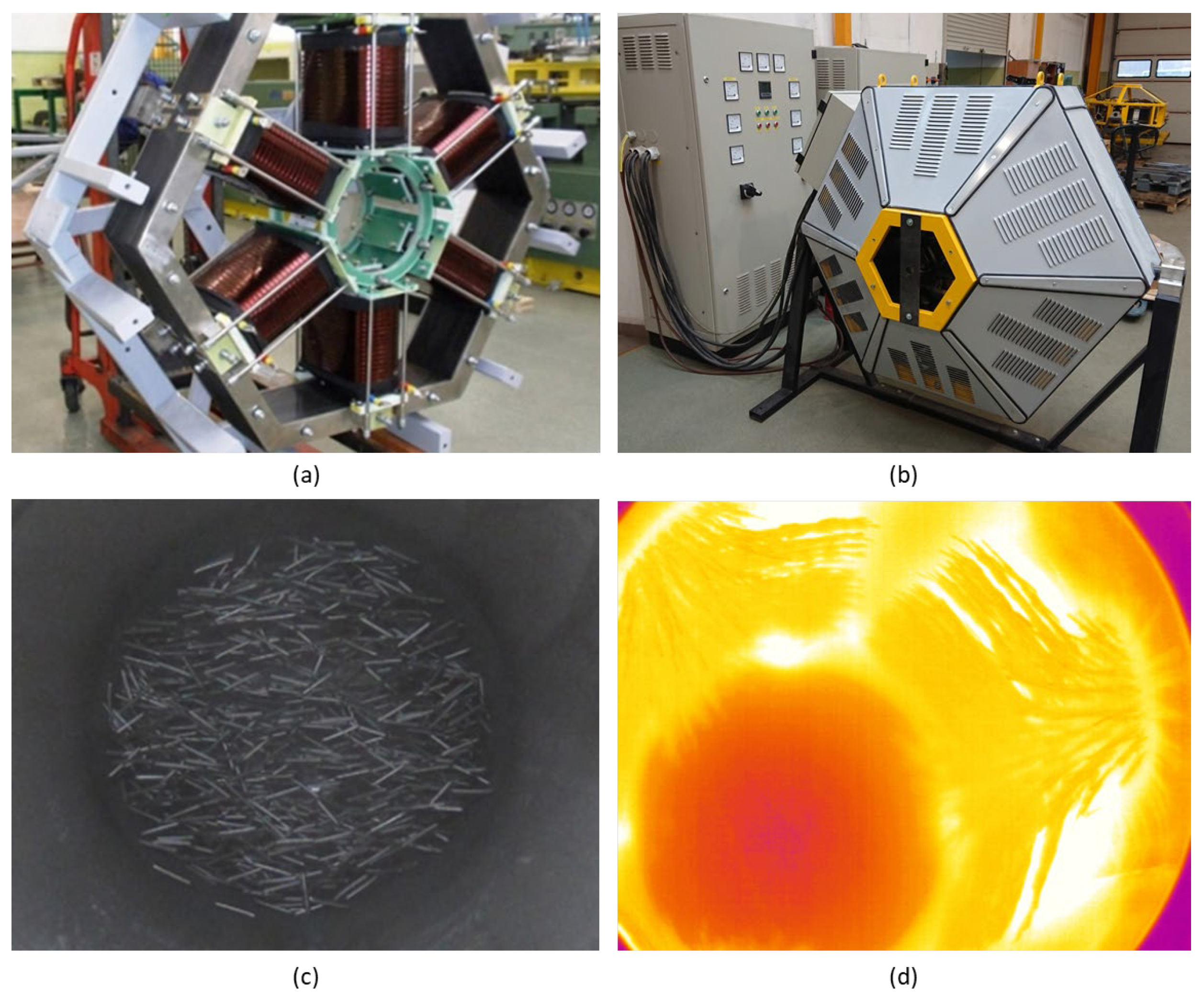
2.1. Construction and Operating Principles of EMM

The electromagnetic mill developed by ELTRAF is a novel grinding device in which a rotating magnetic field directly causes movement of ferromagnetic grinding medium in the working chamber [23]. Figure 1 presents an exemplary D200 EMM with a working chamber diameter equal to 200 mm. The milling process is performed in the working chamber of the mill, which is a non-ferromagnetic tube placed inside the electromagnetic (EM) field inductor. The inductor is composed with three pairs of salient poles placed radially around the working chamber and shifted to each other by an angle of 120° (Figure 1a). After being powered by three-phase grid, they create a rotating magnetic field inside the working chamber, transverse to the chamber length and the direction of the processed material flow. The working chamber is filled with small ferromagnetic rods serving as grinding medium. The size parameters of the rods depend on the mill diameter and the average grain size of the milled material, and are usually 1–3 mm in diameter and 10–15 mm in length. When the rotating magnetic field is inducted in the working chamber, the grinding medium start to move. The processed material is directed to the working chamber, transverse to the grinding medium movement. Material particles collide with the grinding medium when passing through the working chamber what is the main action causing that size reducing of the particles. The rotating magnetic field keeps the grinding medium inside the working chamber, preventing its movement with the processed material stream. Collisions between the rods themselves and with the processed material cause chaotic movements inside the chamber (Figure 1c) and increase the milling effect. At the same time, friction between the rods, material and working chamber walls produces an important amount of heat, further increased by the induced eddy currents. Excessive heat is removed from the system by the air cooling system installed inside the mill’s chassis (Figure 1b) and by the stream of processed material with the transport medium (gas or liquid).
The physical parameters of the mill, including working chamber dimensions, distance between the chamber and inductor, number of inductor cores, etc., were optimized to maximize the force exerted by the electromagnetic field and to minimize the electric energy consumption [23]. It makes the electromagnetic mill highly competitive for other milling solutions.
In this research, EMM is a part of the dry grinding and classification circuit, described in more detail in Section 2.2, equipped with dedicated control system based on PLC and SCADA systems. The EM field inductor of the mill is powered by the Mitsubishi Electric FR—F700 frequency inverter with scalar control [24]. Additionally, the user can change the base frequency fb, which is one of the inverter parameters and corresponds to the rated operating frequency of the motor, if the inverter powers such a motor. Thanks to this, knowing the rated supply voltage, the inverter is able to determine the ratio and change the output voltage in such a way as to maintain its value when the output frequency changes (according to the principle of operation of the scalar control of the inverter) [25].
The frequency inverter allows continuous control and modification of the mill’s operating frequency without any technological breaks, and in turn fast reaction, for processing disturbances (milled material parameters variation, flowrate changes, product quality requirements, etc.). It is one of the most important advantage of EMM when compared to the classic milling solutions, where rotation speed of the drum mills is constant, and its change requires technological downtime and mechanical modifications in the mill’s installation [26].

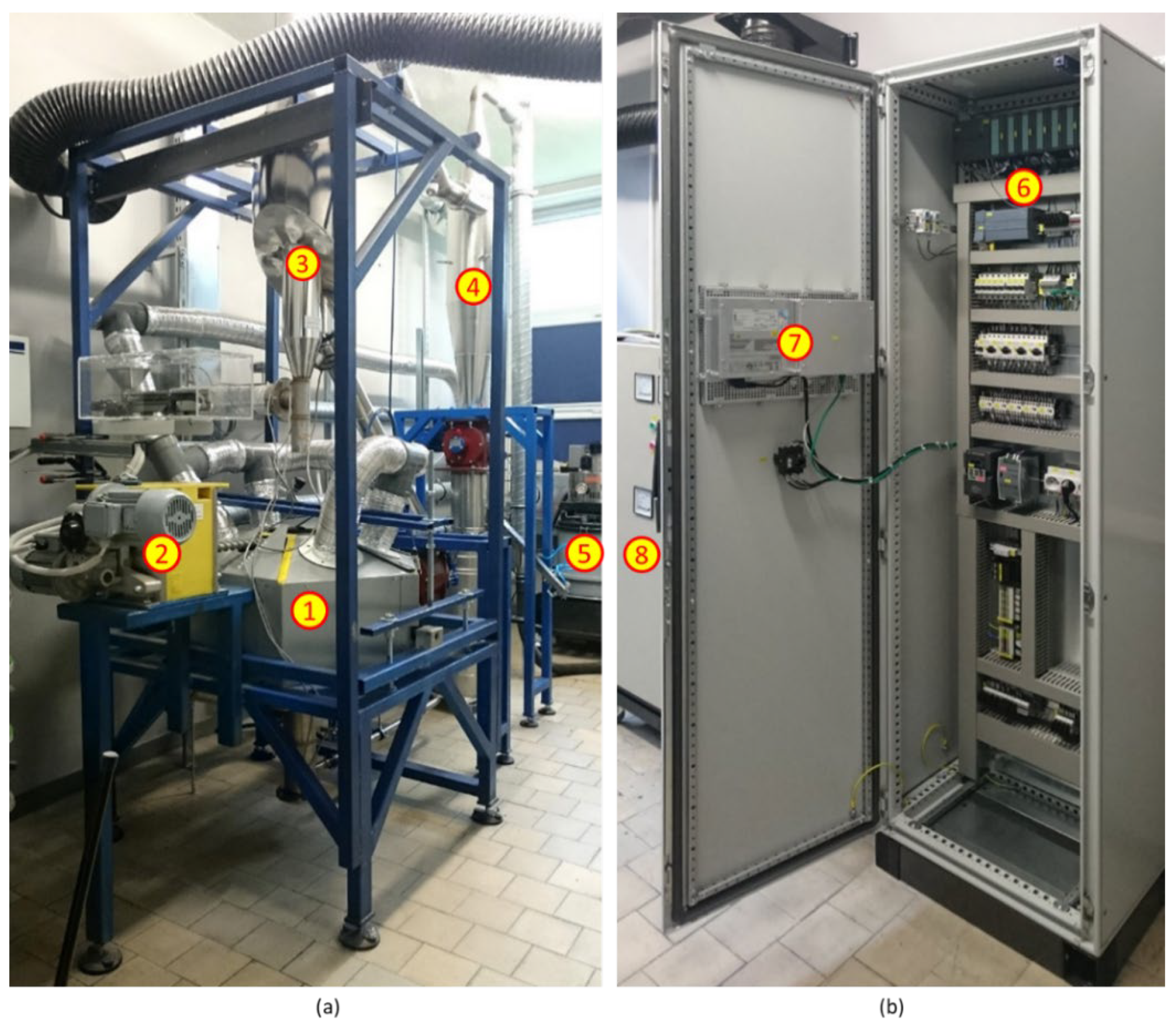
2.2. Semi-Industrial Grinding and Classification Circuit

ELTRAF’s electromagnetic mill is designed to operate in dry and wet batch and continuous milling process. While initial tests for new materials are usually performed in controlled batch experiments, industrial solutions uses dedicated circuits for continuous processes. In this research D100 EMM with 100 mm working chamber diameter is used in the dry grinding and classification circuit located in the Laboratory of Comminution Processes Control at Silesian University of Technology in Gliwice, Poland (see Figure 2). The circuit is designed according to the patented methodology [27] which assumes vertical positioning of the mill and forced air transported movement of the processed material.
In the circuit presented in Figure 2a, the mill (no. 1) is placed horizontally, and the feeding system (no. 2) directs the processed material to the mill from the top of the working chamber. Particles of the material falls by gravity into the working chamber and are kept inside by the transport air stream produced by the negative pressure fan (no. 5), directed from the bottom of the working chamber. The amount of material inside the working chamber (load of the mill) is controlled by dedicated algorithm using indirect acoustic measurement [21]. During milling process the material particles are becoming smaller in size and lighter, and in turn, they start to be moved upwards outside the working chamber into the main classifier (no. 3), which creates two material streams: the product stream (particles with diameter ≤50 µm) and the recycle stream (particles with diameter ≥50 µm) [28]. The product stream is then separated from the air stream in the cyclone (no. 4) and the recycle stream is fed back to the mill from its bottom to ensure additional passing of the particles through the working chamber for the further size reduction.
The whole process is controlled by dedicated power supply and control system presented in Figure 2b. The measurement and control cabinet (no. 6) is equipped with two PLC systems based on SIMATIC S7-300 [29] and SIMATIC S7-1200 [30] controllers with digital and analog I/O modules for communication with sensors and actuators. The system measures transporting air flows, pressures, temperatures and humidities in each supply line of the installation, feed flowrate, electric parameters (voltage, current, active power, etc.), mill load, and mass of the grinding medium inside the working chamber. Research has been performed to improve the system with on-line feed humidity measurements and product quality [31,32]. The system controls the position of damping flaps for the transporting air flow management, process material flowrate and most important—the frequency of the mill operation. S7-1200 controller is connected via MODBUS-RTU communication with Mitsubishi Electric F700 frequency inverter and Lumel ND20 3-phase power network meter [33] installed in the supply cabinet (no. 8). For the purpose of the interaction with the process operator SIMATIC Panel PC [34] was installed and equipped with SCADA system based on GE iFIX platform [35].
The above configuration made it possible to design and implement the multilayered hierarchical control system with dedicated direct control, supervisory control, optimization and production planning layers [36]. Each layer is responsible for specific control tasks, split according to the specific plant sub-systems’ dynamics (control horizons), frequency of disturbances to be attenuated and physical range of the control actions in the plant. The research reported in this paper focus only on the optimization layer actions, so for further discussion it is enough to state that other control layers stabilize the process in the chosen operating point. Control set-points for each sub-system are calculated and distributed by the production planning layer based on the technological requirements.

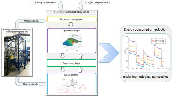
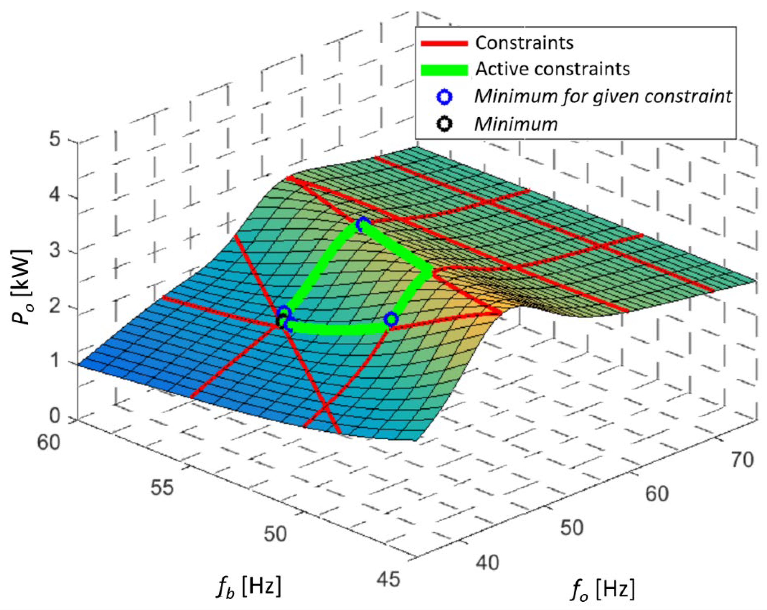
3. Power Optimization Problem

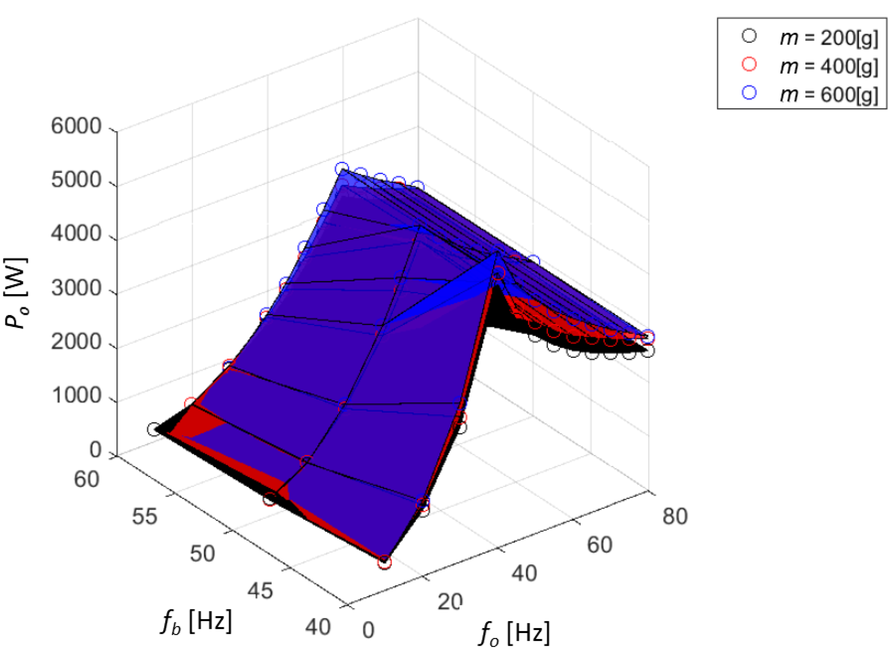
3.1. Objective Function

To maximize profits, one may improve the operation of the distinguished sub-systems of the technological installation. Such division of the global optimization task into separated sub-problems reduces the complexity of the optimization problem; however, the performance of each optimization algorithm should be supervised by an upper-level system that combines all optimization sub-problems into one, and in turn leads to the minimization of the global objective function. This approach is a well-known decomposition of complex optimization tasks, where the coordination of partial optimization tasks takes place by changing the parameters (objective functions and/or constraints) of the partial tasks [37].
In the installation described in Section 3.2, the electromagnetic mill consumes the largest amount of the electrical energy in the system [38]. Thus, it is reasonable to formulate the optimization task as the minimization of the electromagnetic mill active power taking into account quality of the final product and production efficiency.
To formulate the objective function of the optimization problem, a series of tests were required to determine the static active power characteristics of the electromagnetic mill. The dependence of the static characteristic on the mill parameters allows to define decision variables. The mill is supplied by a frequency converter, which output frequency fo and the base frequency fb can be changed. Additionally, the mass of the grinding medium m inside the working chamber may be different as well. To create a static active power characteristic of the mill Po, experiments were carried out in which the output frequency fo and the base frequency fb were changed. Additionally, the experiments were carried out for three different values of the grinding medium mass inside the mill’s working chamber, within the permissible range of grinding medium mass: mi = [200,400,600] g. The experiments were conducted for three values of the base frequency fbj = [40,50,60] Hz, and for changes of the output frequency fo according to the schedule presented in Figure 3. Indices i and j represent the succeeding sample numbers. The active power was measured after reaching steady sate, i.e., 20 s after each change of the frequency set-point.
The results of the experiments are presented in Figure 4. Note that the maximum active power is achieved for the output frequency fo equal to the base frequency fb. Figure 4 also shows obvious dependence on the mass of the grinding medium in the working chamber: power Po rises with mass m. The control system has the ability to change these quantities, which means that they can become decision variables of the optimization problem. Mass m depends, however, on the required product quality and is controlled by a separate system; thus, it can be excluded from the set of decision variables and may be treated as a disturbance that affects the operation of the optimization algorithm. Finally, the following optimization problem is formulated:
m i n f o , f b J f o , f b ,
where the objective function J(fo, fb) is the static characteristic of the mill’s active power (Po). As is further explained, due to the form of the constraints and convexity of J, the analytical model of J is not necessary to be known. For simulation purposes, it is enough to approximate J with non-parametric model, e.g., using Artificial Neural Network (ANN) [39]. There are several ANN models used in this research for approximation of the active power measurements in different working conditions or for approximation of the mill’s supply current measurements. In every instance two-layered neural network was used with one hidden layer. Such structure approximates non-linear characteristic more precisely than one-layered structure [39]. The number of neurons in the hidden layer was determined with the mean square error (MSE) value for measurements approximation. Approximation results were always verified with respect to the expected outcome, consistent with the observed behavior of the device, to avoid over-parametrization of the model. In most cases, seven to ten neurons in the hidden layer were used as a result of the ANN structure design.

3.2. Constraints

In industry, the technological process is always subject to constrains following from product quality requirements, safety condition of the process management, and ensuring failure-free operation. Thus, the allowed area of the J minimum search is always limited by technological constraints.

3.2.1. Product Quality Constraints

The main goal of the control system is to achieve the required production efficiency, expressed by the volume flow of the processed material Ff, and to maintain the assumed quality of the final product. The grinding process product quality is usually assessed by distribution of grain classes, represented by pp vector of percentage content of grain classes in the product, which is obtained for a given set of grain sizes d expressed in mm [28], as for example in (2).
d = 0.05 ,   0.25 ,   0.5 ,   0.57 ,   1 ,   1.5 T   ,
p p = 25 ,   31 ,   31 ,   33 ,   38 ,   48 ,   100 T   ,
Many factors determine the quality of the final product (e.g., feed stream, physical parameters of the ground material, etc.) [40], which means that the vector pp depends on the parameters characterizing the process:
p p = p p Ω ,   F ,   A ,   R ,   M ,
where Ω is a vector containing the output and base frequencies; F is a vector containing parameters of the processed material, such as volumetric flow, density, humidity, temperature, and a vector characterizing the granulation; A is a vector containing the parameters of the transport air flowing through the working chamber, such as volumetric flow, temperature and humidity; R is a vector containing the parameters of the air-material stream flowing through the recycle, i.e., air volume flow, material mass flow and the material grain size vector in recycling; M is a vector containing parameters of the grinding medium such as weight, size and material. It is assumed that the final product quality requirements will be met if the following inequality is met:
p p l p p p p h .
From a multi-level control system point of view, most of the above-mentioned variables cannot be changed by the optimization layer but they are changed by the direct control layer or serves as a technological parameter (treated in the control system as a disturbance). Additionally, only the output and base frequencies (vector Ω) have an impact on both the product quality and the active power, and therefore they become decision variables of the optimization problem. Other values that affect the quality of the product (F, A, R, M) that are not the decision variables should be treated as constant values, depending on the type of material processed or following from the operating point of the plant. The production management layer imposes restrictions on the output frequency fo and the base frequency fb (6) and (7), which make it possible to maintain the desired quality of the final product:
f o l f o f o h ,
f b l f b f b h ,
Constraints (6) and (7) are determined for the certain operating point which is defined by the following set of equations:
F = F O , A = A O , R = R O , M = M O .
If constraints (6) and (7) are met at the system operating point defined by the independent variables (8), then the required quality of the final product is reached. The limit values in (6) and (7) depend on the type of material processed and limit values of (5). In practice, all these limits are determined in laboratory tests and analyzes made by technologists. It is assumed that they are known a priori and are given as the constant parameters of the optimization task.

3.2.2. EMM Voltage Constraint

The electromagnetic mill is equipped with six poles. The pole’s windings have a limited resistance to electric breakdown. This means that they can be supplied with effective voltage Uo not higher than the breakdown voltage Ubrk:
U o U b r k .
The electromagnetic mill is supplied by a scalar-controlled inverter. The inverter changes the output frequency fo, but it changes the mill winding voltage Uo as well. The principle of the scalar control in the case of electric motor power supply is to maintain a constant value of the magnetic flux amplitude in the stator, equal to its value in the nominal operating conditions. The maintenance of the nominal magnetic flux causes the motor to operate under nominal conditions [25]. For this reason, in the inverters with scalar control, the output voltage is changed according to the following equation:
U o = U s u p f o f b ,
where Usup is the supply voltage. Considering the mill supply voltage limitation (9) and Equation (10), it is possible to derive the frequency limitation of the inverter:
f o U b r k U s u p f b .
By introducing the limitation (11) to the optimization problem, the maximum value of the voltage supplying the electromagnetic mill is limited to the level of the breakdown voltage Ubrk.

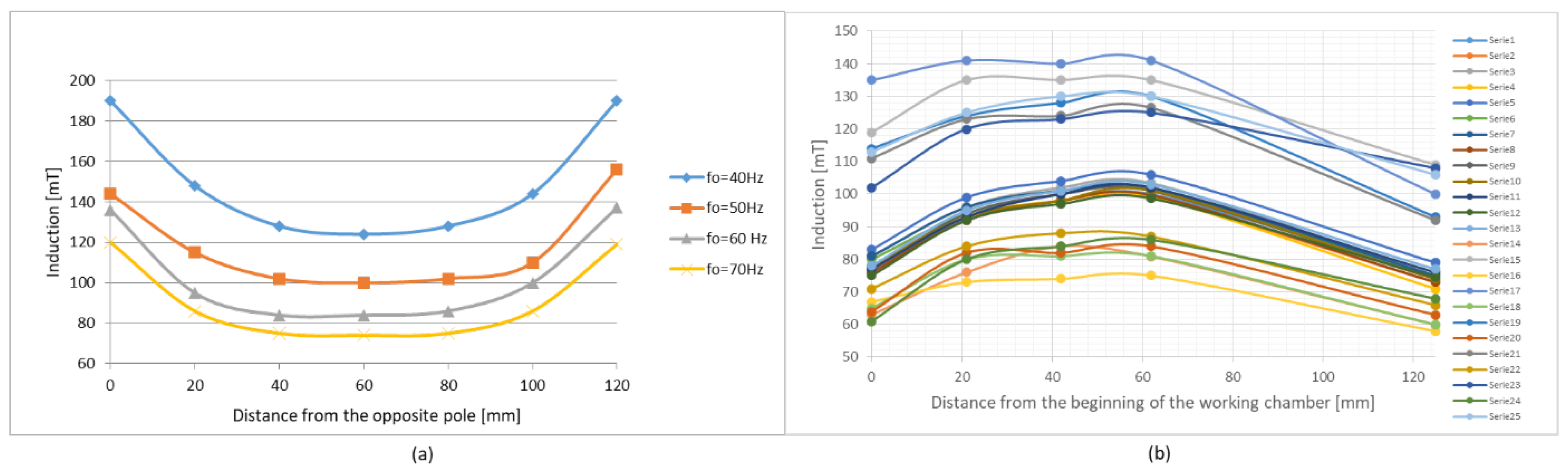
3.2.3. Magnetic Field Induction Constraints

The basic parameter of the electromagnetic mill, which makes it possible to determine the value of the forces acting on the grinding medium in different areas of the working chamber, is the magnetic field induction B [23]. The induction directly impacts the grinding medium movement, and determines its energy to grind a feed. Also, the induction keeps grinding medium vertically in the working chamber. As field quantity, the induction is characterized by its distribution in space, and in particular determines the grinding medium movement [23].
To evaluate the quality of the electromagnetic mill inductor performance, a set of measurements of magnetic induction is carried out at selected points in the mill’s working chamber, not filled with grinding medium or material. Thus, it is possible to measure and model the distribution of induction values in the working chamber space. The measurements are made for different values of the output frequency fo. Figure 5 shows the spatial distribution of the results obtained for the frequency fo = 50 Hz. In Figure 5, the x and y axes define the plane of the cross section of the working chamber, while the z axis is parallel to the side of the working chamber and the induced electromagnetic field rotates around it.
To better illustrate the uniform distribution of induction, it can be presented along a line between opposite poles at an equal distance from the bottom and top of the working chamber (for Dx = 0) (Figure 6a) or along a line parallel to the z axis (or the side edge of the working chamber) (Figure 6b). Figure 6a shows the induction values for fb = 50 Hz and fo = [40,50,60,70] Hz. Figure 6b shows the measurement results for fb = fo = 50 Hz and the respective curves correspond to the points on the cross-section of the working chamber. Exemplary values of the measured induction and respective current Io, as in Figure 6a, are presented in Table 1.
The measurements show that the induction decreases with the distance from the pole front and reaches the minimum Bcentr in the center of the working chamber independently on the frequency fo. For technological reasons, in order to enable the proper movement of the grinding medium to ensure an effective grinding process, it is important to keep the induction over minimum value, therefore it is enough to require:
B c e n t r B m i n ,
where Bmin is the smallest value of magnetic induction for which the grinding medium has sufficient energy to effectively grind the material and keep the grinding medium inside the working chamber. Bmin depends on the physical properties of the processed material. It is important to note that Bmin depends as well on the quantity of grinding medium inside the working chamber and it decreases if this quantity grows [23]. In practice, the Bmin is determined by laboratory experiments or results from the analysis of measurements.
It can be observed in Figure 6 that the induction distribution changes with the change of the output frequency fo. The value of Bcentr is also changing and is smaller, the more the output frequency fo exceeds the value of the base frequency fb, and inversely, if fo is smaller than fb. Table 1 shows that Bcentr increases with the increase of the windings current, which is also shown in Figure 7. Proportional increase of Bcentr in relation to Io is valid only in the range of linear operation of the magnetic circuit. This occurs if the Io does not saturate the magnetic core [23]. Therefore, to limit the magnetic induction Bcentr (12), there is no need to introduce an upper limit on Io of the mill winding. Additionally, the maximum speed of the grinding medium caused by the electromagnetic field is not greater than the frequency of the voltage supplied to the mill [23]. Thus, it is not necessary to introduce an upper limit on the magnetic induction value to keep the upper speed limit of grinding medium (6).
Due to lack of an upper limit on the induction, only the lower limit (12) is valid. Maintaining the limitation (12) requires the determination of the magnetic induction inside the working chamber during the grinding process. It is, howeverr, impossible, because while working, the chamber is filled with grinding medium and material (see Figure 1c). An indirect method should then be used based on the linear relation of induction B and the current Io (see Figure 7). Experimental static characteristic of the current was made depending on the output frequency fo and the base frequency fb for empty working chamber. For the approximation purposes, a two-layer neural network with one hidden layer was used. The two-layer network allows for a more precise approximation of non-linear characteristic [39] then a single-layer variant. To ensure a sufficiently accurate and smooth approximation, a structure with seven neurons in the hidden layer was finally used. The neural network approximator allows to determine the segment where current Io reaches a given value. The experiments with several different materials showed that if the current is greater than 55 A, the limitation of the lower value of the magnetic induction Bmin (12) is kept. The current measurements, as well as the result of the characteristic approximation using ANN and the current limitation, are shown in Figure 8a. The approximation result using linear function of the lower current limitation is shown in Figure 8b.
Finally, the constraints were determined (13) that would make it possible to meet the requirements regarding the minimum value of the magnetic induction in the working chamber (12).
f o a l f b b l f o a p f b b p .
The parameters al, bl, ap, bp in (13) are determined and are constant for a certain type of processed material and can act as guidelines for the fineness and the type of grinding medium used. The parameter values are based on the linear approximation of Io lower limit with the least-squares method [41].

3.3. Optimization Algorithm

Apart from the specification of constraints, the minimization of the mill’s active power requires determination of the objective function J for a given value of the decision variables at a given operating point. This may be the phenomenological model or any form of numerical approximation. Depending on the type of model, appropriate, dedicated methods of searching for the optimal solution are used [37]. The use of complex process models, however, can lead to high computational complexity, which in turn may cause unrealizable algorithms in the context of PLC capabilities. In such a situation, on-line algorithms are often used, where after the decision variables change the value of objective function is directly measured. Such an on-line optimization usually employs directional searching which requires some special analysis of the constraints and assumption of unimodality of the objective function [37].
To illustrate the variability of the objective function J(fo, fb), a family of static characteristics of the active power was created for different mass of grinding medium inside the working chamber. Figure 9 shows the measurement results and approximations of the objective function J(fo, fb). In the discussed case, the objective function is equal to the mill’s active power Po(fo, fb).
Figure 9 shows the measured values of active power Po (represented by the empty circles on the chart), registered by the SCADA system for different set points of base and output frequencies, fb and fo, respectively, and for different mass of grinding medium inside the working chamber m. Based on the measurements models approximating the active power Po were identified for each value of the grinding medium mass m separately. The models were designed as a two-layered ANN with 10 neurons in the hidden layer. Each surface in Figure 9 represents the simulation results for each model separately (e.g., the surface indicating the lowest values of active power is the result of simulation for the model identified for m = 0 g, while the surface indicating the highest values of active power is the result of simulations for model obtained for m = 600 g). Figure 9 shows that for a fixed value of the base frequency fb, there is only one extremum (maximum) of active power for the output frequency fo equal to the base frequency fb. Additionally, in the direction parallel to the base frequency axis fb, the static characteristic is monotonic and decreases with increasing value of the base frequency fb. Therefore, the assumption about unimodality of the static active power characteristic, which is also the objective function of the optimization task J(fo, fb) is met.
Summarizing the conclusions from Section 3.1 and Section 3.2, in particular taking into account (6), (7), (10) and (13), the minimization of the active power of the electromagnetic mill described in Section 2.2 can be achieved by solving the optimization problem written as (1) with respect to the constraints:
45 f o 70 50 f b 55 f o f b f o 1.6 f b 42.4 f o 0.02 f b 60.8 .
The coefficients in (14) are parameters of the optimization problem determined by the supervisory control layer for a given operating point of the technological system. The example presented in (14) concerns the D100 mill, product quality (expressed with 80% of product grains with a size <50 µm) and the process efficiency of 150 kg/h of the processed copper ore. Constraints (14) are graphically presented on the active power static characteristic in Figure 10 to indicate the area where optimum solution will satisfy the constraints. Figure 10 combines the active power measurements (dots) and measurements approximation using the ANN model (surface) with graphical representation of constraints (14). Contrary to Figure 9, it presents only one case of the grinding medium mass (m = 200 g) for clarity. Each line in Figure 10 represents the borders of the allowed area indicated by each constraint, e.g., the area between two red lines (including the lines) represents the region where technological constraints on fo are respected, while the area between two green lines concerns lower limit on Bcentr. Supply voltage requirements, described by only one constraint in (14) are respected in the region on the right side of the black line, representing this constraint. The intersection of all such regions in Figure 10 represents the search area for the optimization task.
The analysis of the objective function J(fo, fb) allows for the choice of the algorithm of searching for the minimum active power of the mill, which ensures the smallest possible effort needed to determine the optimal point. The convexity of the objective function shows that the active power minimum will be located on one of the active constraints that are presented in Figure 10. It is then enough to search only for the active constraints of the optimization problem.
The constraints imposed on the decision variables (fo, fb) are linear (14), which means that a simple one-direction search on the given active constraint may be used to determine the global minimum. There is no need to determine gradient of the objective function, what is the biggest advantage of this approach. Actual value of the objective function can be achieved by changing the output frequency fo and the base frequency fb in the frequency converter supplying the electromagnetic mill, and then measuring the value of the mill’s active power after reaching steady state.
The general outline of the optimization algorithm is presented in the diagram below (Figure 11). The algorithm starts with determining the active constraints (segments A B ¯ ) of the optimization problem. Then, the minimum active power is searched for each segment A B ¯ . The minimum value is stored together with the value of decision variables for which it was obtained. After minimization for each active constraint, the lowest value is selected.
In procedure 1: Determination of active constraints (Figure 11), the active constraints for the i-th step (segments ( A B ¯ i ) are determined by taking the constraint coefficients from the supervisory layer, determining the intersection points of all constraints, selecting points that meet the constraints and creating segments   A B ¯ i .
In procedure 2: Minimizing along the i-th constraint for each of the active constraints, the active power minimum is determined using the golden section method [42]. At the beginning of each iteration of the golden section method, the internal points F1(fo, fb) and F2(fo, fb) are determined at a specific distance from the edge of the segment A B ¯ i obtained from the previous block (No. 1 in Figure 11) according to the golden section rule. The decision variables of point F1 are then set in the inverter. After the active power reaches the steady state, its real value is measured. The whole process is repeated for the point F2. The active power values obtained for both points F1 and F2 are compared and depending on the result of the comparison, one of the constraints of the section A B ¯ i (point A or B) changes and the searching interval is shortened. Each iteration is completed by checking the stop condition (15):
A B i ¯ < ε .
The maximum number of iterations of Iter [37] is also limited according to Equation (16):
Iter Int ln ε ln A 1 B 1 i ¯ ln 0.618 + 1 ,
where A 1 B 1 i ¯ is the initial length of the interval A B ¯ i . Meeting the stop condition (15) or exceeding the maximum number of iterations (16) causes the termination of the golden section method.
Each execution of the optimization algorithm results in a new minimum of the objective function that satisfies all constraints of the optimization problem. The proposed optimization algorithm is insensitive to the change of the operating point due to the measurement of the actual value of active power instead of calculation of the value indirectly through a model. However, in order to verify the algorithm in simulations an approximation of the active power was used by means of an ANN as described in Section 3.1 (Figure 10). The simulated process of searching for the minimum is presented in the diagram in Figure 12.
It can be seen that with each iteration of the golden section method, the decision variables tend to the minimum value of each constraint, narrowing the segment A B ¯ i . Finally, a minimum is determined for each constraint (Figure 13) and the lowest value is selected. The starting point for the simulated optimization task is the set of nominal frequencies fo = fb = 50 Hz resulting in the active power Po value over 3.6 kW. As Figure 13 shows, the optimization algorithms is calculating the lowest values of the objective function (equal to active power) for each of the active constraints (blue circles). Then, the overall minimum is chosen from all solution candidates (black circle) resulting in the active power reduction to almost 2.1 kW that stands for almost 42% of the power reduction. As follows from the analysis of the objective function model in Figure 13, further reduction of active power is possible, e.g., for lower values of fo. It would, however, lead to the violation of the imposed technological and quality constraints, hence only the allowed area inside the constrained region can be considered.

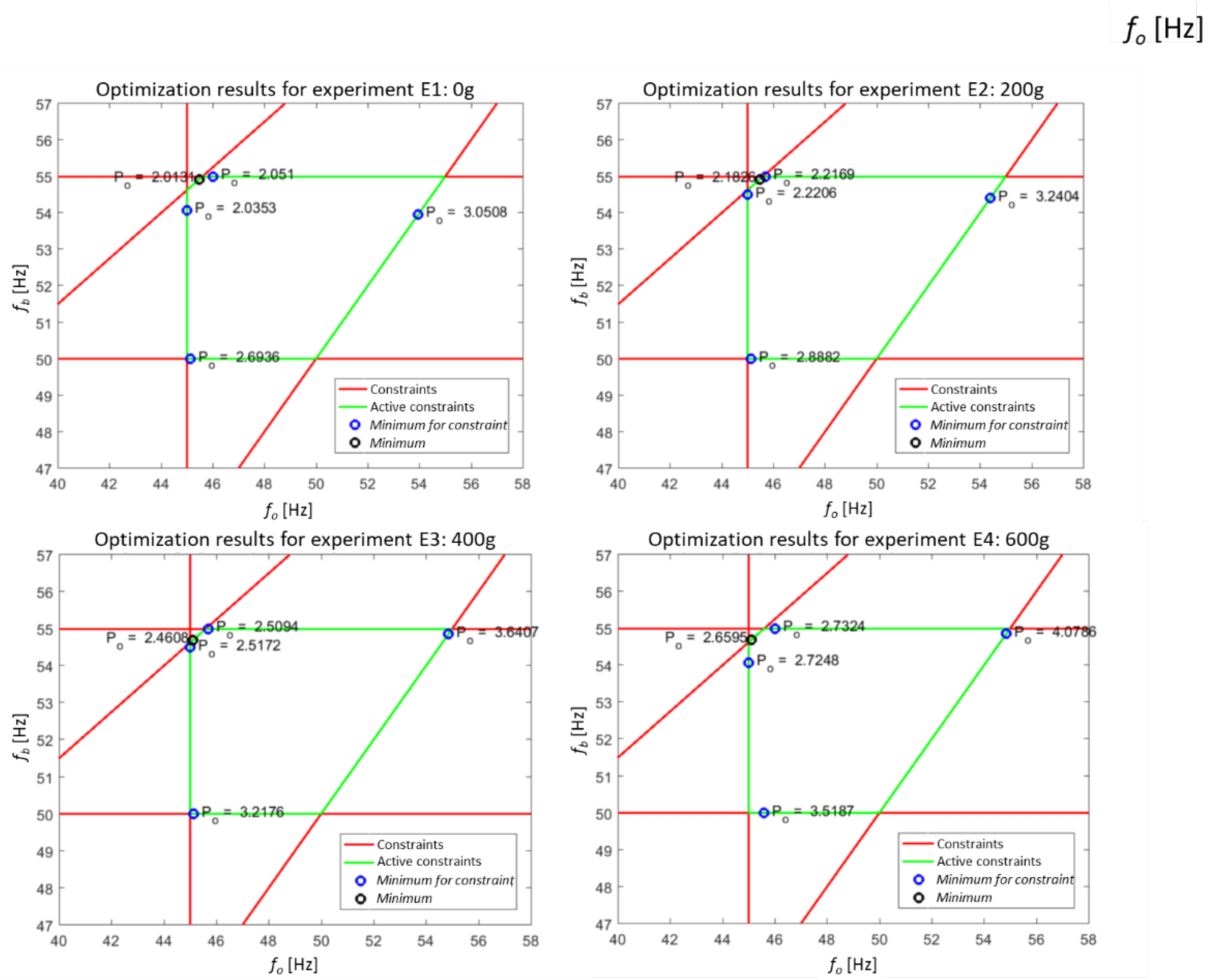
4. Algorithm Validation in Semi-Industrial Tests

4.1. Algorithm Implementation

Since the algorithm is based on the measurement of active power, the measurement resolution and measurement noise, as well as the resolution of setting the base frequency fb and the output frequency fo, should be taken into account. Interactions between these resolutions and the noise range determines the parameter ε choice, which is the stop condition of the optimization task (15). For the tested installation with the D100 mill and Mitsubishi F700 inverter, the value of the stop condition was determined as ε = 1.
Another extremely important aspect is the dynamics of the object, i.e., the dynamics of technological changes in the entire installation, and the dynamics of the control path. The inverter used was parameterized to ensure a frequency change in the range of 0–50 Hz within 3 s. Taking this parameter into account, as well as the settling time of the active power and necessary time to execute the optimization algorithm, the sampling time was set to Topt = 30 s. The algorithm was implemented on the PC panel in a SCADA application using the VBA language.
The series of experiments was carried out for various operating points of the installation after implementing the optimization algorithm. From an energy consumption point of view, the key sensitivity of the operating point concerns change of the grinding medium mass in the working chamber. Grinding medium mass follows from technological requirements and depends, inter alia, on the average mill throughput, the type of processed material and requirements on the grinding ratio (average size reduction factor). Such tests made it possible to assess the applicability of the proposed algorithm for a wide range of technological scenarios.

4.2. Results of Experiments

As part of many tests, four experiments E1 to E4 were carried out, in which a mass of grinding medium mk = [0,200,400,600] g was checked. Figure 14 summarizes the time series of these experiments: the range of changes in the base and output frequencies and the change in active power of the mill.
The charts in Figure 14 show that the selected sampling period allows the active power signal to reach a steady state before the succeeding step of the optimization algorithm is performed. The values of the algorithm parameters were also correctly selected to give the algorithm smooth converge. Note that the change of the operating point does not affect the algorithm efficiency. Obviously, the change in the grinding medium mass has an impact on the average value of the active power, which is the expected effect.
Analysis of the results shows that for each of the active constraints, the method determines the minimum of the objective function and then selects the one for which this value is the lowest. The results of the algorithm for four experiments are presented in Figure 15. For each operating point, the method determined the values of the fb and fo frequencies, minimizing the energy consumption, which each time is lower by approximately 40% than the value obtained for the nominal settings fb = 50 Hz and fo = 50 Hz (compare Figure 14b).

4.3. Discussion of Results

The obtained results show that the proposed optimization algorithm enables the minimization of energy consumption by the electromagnetic mill while maintaining the constraints imposed on the process. Similar global minimums follow from the same set of constraints applied in each experiment. In industrial production scenarios, such important changes in the grinding medium mass would usually be combined with different technological requirements for the final product and, in turn, affect the parameters of the imposed constraints. Such modification during experimental verification of the proposed algorithm were not introduced on purpose to allow a clear comparison of results. On-line optimization algorithm was successfully verified; however, the process of searching for the minimum along the active constraint requires many changes of decision variables, which may disrupt the grinding operation.
The reduction of the negative impact of the proposed method can be achieved by carrying out each iteration of the optimization algorithm in an appropriate time window. Time needed to carry out the entire optimization process should be adjusted to the dynamics of disturbances affecting the electromagnetic mill (e.g., changes in the mass of grinding medium, changes in the physical parameters of the feed) so that the determination of the minimum active power follows the change in the operating point of the technological system. The frequency variation can also affect the quality of the final product, whereby in the case of searching and keeping the constraints, the required quality will not be affected.
Frequent changes in the output and base frequencies affect the service life of the actuators. The number of changes in decision variables can be limited by the appropriate modification of the parameter ε. However, the value of this parameter affects the accuracy of the determination of the minimum location. The number of changes also depends on the length of the segment A B ¯ , representing a given active constraint and it becomes smaller the shorter the length of this segment is.

5. Conclusions

The article presents a practical solution to the problem of minimizing electrical energy consumption by the electromagnetic mill. It has been shown that using two variables (output frequency and base frequency) to determine the operation of the inverter makes it possible to change the active power of the electromagnetic mill–inverter system. The search for minimal consumption was shown using the static characteristic of the mill’s active power versus the output and base frequency and the mass of grinding medium inside the working chamber. After approximation of the static characteristics with a two-layer neural network, it was possible to analyze the influence of the output frequency, base frequency and grinding medium mass on the active power of the electromagnetic mill. For technological reasons, both frequencies were selected as the two decision variables for the optimization task.
Analysis of the output and base frequencies was carried out, taking into account the quality of the final product. It was noticed that the change in the base frequency caused a change in the supply voltage of the mill coils, which, in the absence of the internal inverter limitation, may lead to their damage. Also shown is the indirect influence of decision variables on the magnetic flux of the working chamber, which determines the ability of the grinding medium to grind the material and keep them inside the working chamber. As a result, the optimization task objective function was designed with the set of technological and construction constraints. Satisfying the constraints makes it possible to keep the required quality of the final product, enables failure-free operation of the mill coils, and finally, creates magnetic field intensive enough to hold the grinding medium inside the working chamber while rotating fast enough to break the feed grains.
Convexity of the objective function was confirmed by experimental measurements and allows to created effective optimization algorithm which searches minima of the active power of the mill on the active constraints. The proposed optimization algorithm finds the global minimum of the active power, regardless of the operating point of the technological system. The efficiency of the proposed on-line optimization algorithm was successfully verified during experiments on a dry grinding installation with an electromagnetic mill D100. Further research will focus on constraint modification, e.g., using additional information on the product quality based on the on-line product grain sizes measurement.

Funding

The research reported in this paper was performed on installation co-financed by the National Centre for Research and Development, Poland, under Applied Research Programme, project number PBS3/B3/28/2015 (acronym SYSMEL). The APC was funded by the rector’s habilitation grant, Silesian University of Technology, grant number 02/050/RGH20/0014.

Institutional Review Board Statement

Not applicable.

Informed Consent Statement

Not applicable.

Data Availability Statement

Data sharing not applicable.

Acknowledgments

The author would like to acknowledge a vital role of Markus Swierzy (member of the SYSMEL team) in preparing and conducting the experiments.

Conflicts of Interest

The author declares no conflict of interest. The funders had no role in the design of the study; in the collection, analyses, or interpretation of data; in the writing of the manuscript, or in the decision to publish the results.

References

  1. Wills, B.A.; Napier-Munn, T. Comminution. In Wills’ Mineral Processing Technology; Butterworth-Heinemann: Oxford, UK, 2005; Chapter 5; pp. 108–117. [Google Scholar]
  2. Fuerstenau, M.C.; Han, K.N. Principles of Mineral Processing; SME: Chicago, IL, USA, 2003. [Google Scholar]
  3. Mular, A.L.; Doug, N.H.; Derek, J.B. Mineral Processing Plant Design. Practice and Control Proceedings; SME: Chicago, IL, USA, 2002. [Google Scholar]
  4. Leistner, T.; Peuker, U.A.; Rudolph, M. How Gangue Particle Size Can Affect the Recovery of Ultrafine and Fine Particles During Froth Flotation. Miner. Eng. 2017, 109, 1–9. [Google Scholar] [CrossRef]
  5. Wang, Y.; Forssberg, E. Enhancement of energy efficiency for mechanical production of fine and ultra-fine particles in comminution. China Particuol. 2007, 5, 193–201. [Google Scholar] [CrossRef]
  6. Jeswiet, J.; Szekeres, A. Energy consumption in mining comminution. Procedia CIRP 2016, 48, 140–145. [Google Scholar] [CrossRef] [Green Version]
  7. Fuerstenau, D.; Abouzeid, A.Z. The energy efficiency of ball milling in comminution. Int. J. Miner. Process. 2002, 67, 161–185. [Google Scholar] [CrossRef]
  8. Walkiewicz, J.; Clark, A.; McGill, S. Microwave-assisted grinding. IEEE Trans. Ind. Appl. 1991, 27, 239–243. [Google Scholar] [CrossRef]
  9. Musa, F.; Morrison, R. A more sustainable approach to assessing comminution efficiency. Miner. Eng. 2009, 22, 593–601. [Google Scholar] [CrossRef]
  10. Hesse, M.; Popov, O.; Lieberwirth, H. Increasing efficiency by selective comminution. Miner. Eng. 2017, 103, 112–126. [Google Scholar] [CrossRef]
  11. Wang, Y.M.; Forssberg, E. New Milling Technology. Technical Report; MinFo: Stockholm, Sweden, 2001. [Google Scholar]
  12. Grimble, M.J. Industrial Control System Design; Wiley: Hoboken, NJ, USA, 2001. [Google Scholar]
  13. Hodouin, D. Methods for automatic control, observation, and optimization in mineral processing plants. J. Process Control 2011, 21, 211–225. [Google Scholar] [CrossRef]
  14. Simon, J.; Guélou, G.; Srinivasan, B.; Berthebaud, D.; Mori, T.; Maignan, A. Exploring the thermoelectric behavior of spark plasma sintered Fe7-xCoxS8 compounds. J. Alloy. Compd. 2020, 819, 152999. [Google Scholar] [CrossRef]
  15. Lokiec, H.; Lokiec, T. Inductor of Electromagnetic Mill. Polish Patent No. PL 226554 B1, 19 May 2015. (In Polish). [Google Scholar]
  16. Electromagnetic Mill. Available online: https://globecore.com/products/magnetic-mill/ (accessed on 10 March 2021).
  17. Styla, S. Laboratory studies of an electromagnetic mill inductor with a power source. Int. Q. J. Econ. Technol. Model. Process. 2017, 6, 109–114. [Google Scholar]
  18. Styla, S. New Grinding Technology Using an Electromagnetic Mill–Testing the Efficiency of the Process. Int. Q. J. Econ. Technol. Model. Process. 2017, 6, 81–88. [Google Scholar]
  19. Calus, D.; Makarchuk, O. Analysis of interaction of forces of working elements in electromagnetic mill. Przeglad Elektrotechniczny 2019, 1, 64–69. [Google Scholar] [CrossRef]
  20. Makarchuk, O.; Calus, D.; Moroz, V. Mathematical model to calculate the trajectories of electromagnetic mill operating elements. Tekhnichna Elektrodynamika 2021, 2, 26–34. [Google Scholar] [CrossRef]
  21. Ogonowski, S.; Ogonowski, Z.; Swierzy, M.; Pawelczyk, M. Control system of electromagnetic mill load. In Proceedings of the 25th International Conference on Systems Engineering, Las Vegas, NV, USA, 22–24 August 2017; pp. 69–76. [Google Scholar] [CrossRef]
  22. Ogonowski, S.; Ogonowski, Z.; Pawelczyk, M. Multi-objective and multi-rate control of the grinding and classification circuit with electromagnetic mill. Appl. Sci. 2018, 8, 506. [Google Scholar] [CrossRef] [Green Version]
  23. Sosinski, R. Opracowanie Metodyki Projektowania Trójfazowych Wzbudników z Biegunami Jawnymi Pola Wirującego do Młynów Elektromagnetycznych (Development of Design Methodology for three-Phase Salient-Pole Exciters of Rotating Field for Electromagnetic Mills—In Polish). Ph.D. Thesis, Czestochowa University of Technology, Czestochowa, Poland, 2006. [Google Scholar]
  24. Mitsubishi Electric F700 Inverter Instruction Manual. Available online: https://dl.mitsubishielectric.com/dl/fa/document/manual/inv/ib0600177eng/ib0600177engf.pdf (accessed on 10 March 2021).
  25. Kabzinski, J. Advanced Control of Electrical Drives and Power Electronic Converters; Springer International Publishing AG: Cham, Switzerland, 2017; ISBN 978-3-319-83362-0. [Google Scholar]
  26. Goralczyk, M.; Krot, P.; Zimroz, R.; Ogonowski, S. Increasing Energy Efficiency and Productivity of the Comminution Process in Tumbling Mills by Indirect Measurements of Internal Dynamics—An Overview. Energies 2020, 13, 6735. [Google Scholar] [CrossRef]
  27. Pawelczyk, M.; Ogonowski, Z.; Ogonowski, S.; Foszcz, D.; Saramak, D.; Gawenda, T.; Krawczykowski, D. Method for Dry Grinding in Electromagnetic Mill. Polish Patent PL 413041, 6 June 2015. [Google Scholar]
  28. Wolosiewicz-Glab, M.; Ogonowski, S.; Foszcz, D.; Gawenda, T. Assessment of classification with variable air flow for inertial classifier in dry grinding circuit with electromagnetic mill using partition curves. Physicochem. Probl. Miner. Process. 2018, 54, 440–447. [Google Scholar] [CrossRef]
  29. SIMATIC S7-300. Available online: https://new.siemens.com/global/en/products/automation/systems/industrial/plc/simatic-s7-300.html (accessed on 10 March 2021).
  30. SIMATIC S7-1200. Available online: https://new.siemens.com/global/en/products/automation/systems/industrial/plc/s7-1200.html (accessed on 10 March 2021).
  31. Buchczik, D.; Wegehaupt, J.; Krauze, O. Indirect measurements of milling product quality in the classification system of electromagnetic mill. In Proceedings of the 22nd International Conference on Methods and Models in Automation and Robotics, Miedzyzdroje, Poland, 28–31 August 2017; pp. 1039–1044. [Google Scholar] [CrossRef]
  32. Budzan, S.; Buchczik, D.; Pawelczyk, M.; Tuma, J. Combining Segmentation and Edge Detection for Efficient Ore Grain Detection in an Electromagnetic Mill Classification System. Sensors 2019, 19, 1805. [Google Scholar] [CrossRef] [PubMed] [Green Version]
  33. LUMEL 1 and 3-Phase Power Network Meter ND20. Available online: https://www.lumel.com.pl/en/catalogue/product/1-and-3-phase-power-network-meter-nd20 (accessed on 10 March 2021).
  34. SIMATIC IPC 477D Panel PC. Available online: https://mall.industry.siemens.com/mall/en/WW/Catalog/Product/?mlfb=6AV7240-6BD17-0PA2 (accessed on 10 March 2021).
  35. GE Digital Proficy HMI/SCADA iFIX. Available online: https://www.ge.com/digital/applications/hmi-scada/ifix (accessed on 10 March 2021).
  36. Tatjewski, P. Advanced Control of Industrial Processes: Structures and Algorithms; Springer: London, UK, 2007. [Google Scholar]
  37. French, M. Fundamentals of Optimization; Springer International Publishing AG: Cham, Switzerland, 2018; ISBN 978-3-319-76191-6. [Google Scholar]
  38. Ogonowski, S.; Ogonowski, Z.; Swierzy, M. Power optimizing control of grinding process in electromagnetic mill. In Proceedings of the 21st International Conference on Process Control, Strbske Pleso, Slovakia, 6–9 June 2017; pp. 370–375. [Google Scholar] [CrossRef]
  39. Braspenning, P.J.; Thuijsman, F.; Weijters, A.J.M.M. Artificial Neural Networks. An Introduction to ANN Theory and Practice; Springer: Berlin/Heidelberg, Germany, 1995; ISBN 978-3-540-59488-8. [Google Scholar]
  40. Krauze, O.; Buchczik, D.; Budzan, S. Measurement-Based Modelling of Material Moisture and Particle Classification for Control of Copper Ore Dry Grinding Process. Sensors 2021, 21, 667. [Google Scholar] [CrossRef] [PubMed]
  41. Wolberg, J. Data Analysis Using the Method of Least Squares: Extracting the Most Information from Experiments; Springer: Berlin/Heidelberg, Germany, 2006; ISBN 978-3-540-25674-8. [Google Scholar]
  42. Kiefer, J. Sequential minimax search for a maximum. Proc. Am. Math. Soc. 1953, 4, 502–506. [Google Scholar] [CrossRef]
Figure 1. Electromagnetic mill D200: (a) inductor; (b) mill on the test stand without the working chamber; (c) ferromagnetic rods (grinding medium) moving inside the working chamber; (d) grinding medium during stop procedure arranging according to the pole lines (thermo-vision image).
Energies 14 02380 g001
Figure 2. Semi-industrial dry grinding and classification circuit with EMM D100: (a) installation with air transport and heat recovery systems; (b) control and power supply cabinets.
Energies 14 02380 g002
Figure 3. Schedule of the output frequency fo changes during identification experiments.
Energies 14 02380 g003
Figure 4. Static characteristic of the active power versus output and basic frequencies obtained for different mass of grinding medium.
Energies 14 02380 g004
Figure 5. Distribution of the measured value of the magnetic induction inside the mill’s working chamber. Dx and Dy are the distance in mm from the center of the working chamber, while Dz is the distance from the bottom (beginning) of the working chamber. The value of the induction in mT is marked with the appropriate color, shown in the legend.
Energies 14 02380 g005
Figure 6. Distribution of the measured value of the magnetic induction inside the working chamber: (a) along a line between opposite poles; (b) along lines parallel to the side edge of the working chamber (each series represents different measuring point on the working chamber cross-section).
Energies 14 02380 g006
Figure 7. Magnetic induction measured in the center of the working chamber in the function of the windings current.
Energies 14 02380 g007
Figure 8. (a) The current and its approximation by ANN; (b) the current limitation and its linear approximation.
Energies 14 02380 g008
Figure 9. Approximation of the static active power characteristic of the mill depending on the grinding medium mass.
Energies 14 02380 g009
Figure 10. Constraints on the static characteristics of the active power of the inverter.
Energies 14 02380 g010
Figure 11. General form of the optimization algorithm.
Energies 14 02380 g011
Figure 12. Simulation of searching for the minimum active power by directional optimization on the active constraints.
Energies 14 02380 g012
Figure 13. Simulation result of the proposed optimization algorithm.
Energies 14 02380 g013
Figure 14. Results of experiments for various mass of grinding medium: (a) changes in frequency values; (b) changes in the active power of the mill (objective function).
Energies 14 02380 g014
Figure 15. The results obtained from the optimization algorithm for the experiments with different mass of grinding medium.
Energies 14 02380 g015
Table 1. Measured values of magnetic induction B for different output frequencies fo and measured output current Io.
Distance from PoleMagnetic Induction B [mT]
LeftRightfo = 40 Hzfo = 50 Hzfo = 60 Hzfo = 70 Hz
x [mm ]x’ [mm]Io = 90 AIo = 68 AIo = 56 AIo = 49 A
0120190144136120
201001481159586
40801281028475
60601241008474
80401281028675
1002014411010086
1200190156137119
Publisher’s Note: MDPI stays neutral with regard to jurisdictional claims in published maps and institutional affiliations.

