Support Vector Machine Based Fault Location Identification in Microgrids Using Interharmonic Injection

Abstract

This paper proposes an algorithm for detection and identification of the location of short circuit faults in islanded AC microgrids (MGs) with meshed topology. Considering the low level of fault current and dependency of the current angle on the control strategies, the legacy overcurrent protection schemes are not effective in in islanded MGs. To overcome this issue, the proposed algorithm detects faults based on the rms voltages of the distributed energy resources (DERs) by means of support vector machine classifiers. Upon detection of a fault, the DER which is electrically closest to the fault injects three interharmonic currents. The faulty zone is identified by comparing the magnitude of the interharmonic currents flowing through each zone. Then, the second DER connected to the faulty zone injects distinctive interharmonic currents and the resulting interharmonic voltages are measured at the terminal of each of these DERs. Using the interharmonic voltages as its features, a multi-class support vector machine identifies the fault location within the faulty zone. Simulations are conducted on a test MG to obtain a dataset comprising scenarios with different fault locations, varying fault impedances, and changing loads. The test results show that the proposed algorithm reliably detects the faults and the precision of fault location identification is above 90%.

1. Introduction

The increasing penetration of distributed energy resources (DERs) in electrical grids gives rise to new problems concerning the operation, control, and protection of electrical networks. A systematic approach for dealing with these issues is to regard a set of interconnected DERs and local loads as a microgrid (MG) [1]. A MG can be connected to the main grid or operate in islanded operation mode. During the grid-connected operation mode, the power exchange between the MG and the network can be managed based on economic and technical requirements. The MG can be disconnected from the main grid either intentionally or in response to occurrence of a disturbance or power outage in the main grid to ensure uninterruptible power delivery to the local loads. Although MGs favor improved reliability and controllability, the coordination of protection systems in a MG is a challenging problem. In contrast with the conventional distribution networks, in which the fault current is usually unidirectional, bidirectional fault currents are common in MGs owing to the presence of DERs. In addition, the fault current level in an MG significantly varies in different operation modes (grid-connected/islanded) and is highly dependent on the network structure [2].

The legacy protection schemes of distribution systems are not effective against bidirectional fault currents in MGs. Furthermore, the contribution of DERs to the fault current alters the trip time of protection devices, which in turn deteriorates the coordination among them [3]. For instance, in the conventional fuse saving scheme, as long as the fault current is within a specific range, the reclosers trip faster than the fuses. The contribution of DERs to fault current might result in increasing the fault current beyond this range, hence causing the fuse to burn even during temporary faults [4]. Another factor that adversely affects the coordination is the dynamic nature of MGs’ topology. A MG’s topology might change owing to the interconnection of new DERs and new loads, the change of operation mode, or planned/unplanned maintenance.

A simple approach for circumventing the mentioned issues is to quickly disconnect the DERs upon the occurrence of a fault. This way, the legacy protection schemes will remain to be effective and issues such as blinding protection and sympathetic tripping are prevented [5]. However, the disconnection of DERs results in decreasing the grid voltage during fault conditions and might eventually lead to instability when the DER penetration is high. To prevent the mentioned issues, fault current limiters can be employed to limit the impact of DERs on the legacy protection scheme [6]. Passive fault current limiters are series reactors that are permanently in circuit. As they give rise to voltage deviations during normal operation, their application is quite limited [7]. Active fault current limiters utilize thyristors to realize a variable impedance, which is small during normal operation, but increases to large values during fault to limit the fault current. The main shortcoming of fault current limiters is their high cost, which limits their practical application [8].

Considering the aforementioned issues, the development of protection schemes with consideration of the impact of DERs and grid topology variations seems crucial. To that end, numerous MG protection schemes based on computational intelligence and machine learning approaches, such as fuzzy systems, multi-agent systems, artificial neural networks, and metaheuristics, have been proposed [9]. Fuzzy systems have been adopted in [10,11] to implement adaptive protection schemes, which alter the relay set-points in response to variations in the MG operation mode and the network topology. A multi-agent protection scheme has been proposed in [12], in which several agents including a measurement agent, breaker agent, optimal coordination agent, and protection agent cooperate to realize an adaptive protection scheme. Machine learning-based protection approaches detect short circuit faults by analyzing certain features, which are extracted from the measured voltages and current [13]. Various signal processing methods such as wavelet transform [13], transform [14], and Hilbert–Huang transform [15] are employed to extract the features of measured signals and indicate the features with useful information regarding faults. The selected features are then used as inputs of a machine learning algorithm to detect the fault. In [16], Fourier transform is used to extract the useful features, which are then applied to a decision tree to detect and identify the type of fault. In [16], after extracting the features using Hilbert–Huang transform, they are used by three different types of classifiers (naive classifier, support vector machine (SVM), and extreme learning machine classifier) to distinguish the fault type. In [13], discrete wavelet transform is used along with extreme machine learning classifier to identify the faulty section as well as the fault type. A radial basis function neural network is used in [17] for the detection of fault location. Hence, the faulty line is determined and then the protection devices are coordinated by backtracking technique. In [18], an interharmonics injection-based protection scheme is presented for identification of fault location in MGs. In this method, the DERs that are electrically closer to the fault inject interharmonics currents at different frequencies into the grid. The fault location is then obtained using an SVM classifier.

The pre-requisite for the implementation of machine-learning-based protection schemes is training the “machine” with a dataset. This dataset is commonly generated by running a large number of simulations with various fault scenarios. The existing machine learning-based protection schemes [9,10,11,12,13,14,15,16,17,18] are mostly focused on detection of faults with a small fault impedance. That is to say, they only consider scenarios in which the fault impedance is small during the training stage and validate their algorithms by the same small fault impedances. In addition, most of the existing machine learning-based protection schemes have not considered the effect of load variations in training and test scenarios. In practice, the fault impedance depends on the cause of fault and may vary in a large range. For higher fault impedances, the detection of fault location and identification of its location become more difficult. Furthermore, the load has a stochastic nature and changes all the time. So, consideration of low fault impedance and fixed load is an oversimplification of the problem, which enables the existing methods to obtain very good, but unrealistic results.

In this paper, an SVM-based algorithm is proposed for the detection and identification of the location of three phase short circuit faults in meshed MGs. Owing to the limited ac current rating of DERs, their output voltage experiences a significant drop during the fault condition. In the proposed scheme, the SVM detects the occurrence of fault based on the rms voltage of the DERs. Once a fault is detected, selected DERs inject a few interharmonics currents into the grid. By investigating the flow of interharmonics currents in different paths, the fault current is tracked, and hence the fault zone is identified. In the last stage, the faulty line is detected by a multiclass support vector machine (MSVM) based on the measured voltage interharmonics at DERs terminals. The proposed scheme considers both load and fault impedance variations throughout training and testing stages.

The main contributions of the paper are listed below.

• An interharmonic injection method is proposed to enable detection of fault location in meshed microgrids. By appropriate selection of interharmonic amplitudes and proper design of the control loops, it is ensured that the interharmonic voltages are not suppressed owing to the action of the DER current limiting mechanism or absorption by other DERs. So, unlike the fundamental component, interharmonic voltages are representative of the impedance seen by the DER, and hence can be used for finding the fault location. Moreover, as the interharmonics are only injected after detection of a fault, they do not have any impact on the normal operation of the MG.
• An MSVM classifier is used to detect the faulty line based on measured interharmonic voltages at DER terminals. Unlike the method of [18], the proposed MSVM is trained and tested by considering various loading and fault impedance scenarios.
• The impact of fault impedance and load variations on the accuracy of the proposed algorithm is investigated. It is shown that, by injecting several interharmonics from each DER, the accuracy can be significantly improved compared with the single interharmonic injection strategy [18].

2. Proposed Fault Detection Strategy

In contrast with the legacy distribution networks, in which fault is detectable by overcurrent relays, overcurrent protection is not effective in islanded MGs owing to the low value of fault current level. This is mainly caused by the limited capacity of DERs, which utilize a current limiting mechanism to prevent overcurrent stresses on inverter switches. During fault condition, the current limiting mechanism controls the current by reducing the DER’s output voltage. As a result, the MG voltage experiences a significant drop, which depends on the fault resistance (R_f). Therefore, the voltage level is a good tool for fault detection.

After the detection of the fault, the fault location should be identified. This task is especially difficult in a meshed MG owing to the low level of fault current impact of load variations and control method of DERs on the current flow during fault and the possibility of current flow from different paths. An efficient technique for dealing with this problem is interharmonic injection [18]. In this method, selected DERs inject interharmonic currents with the frequency f = (n + 1/2)f₀ into the grid. Then, the interharmonic currents and voltages are measured and used for identification of fault location. This technique has some key advantages. First of all, as opposed to the fundamental voltages and currents, the interharmonics are not affected by the current limiting mechanism of the DERs. Secondly, by utilizing different interharmonic frequencies for each DER, the fault current paths can be easily identified. Thirdly, by utilizing multiple interharmonic frequencies, more extensive information can be obtained, which allows enhancing the accuracy.

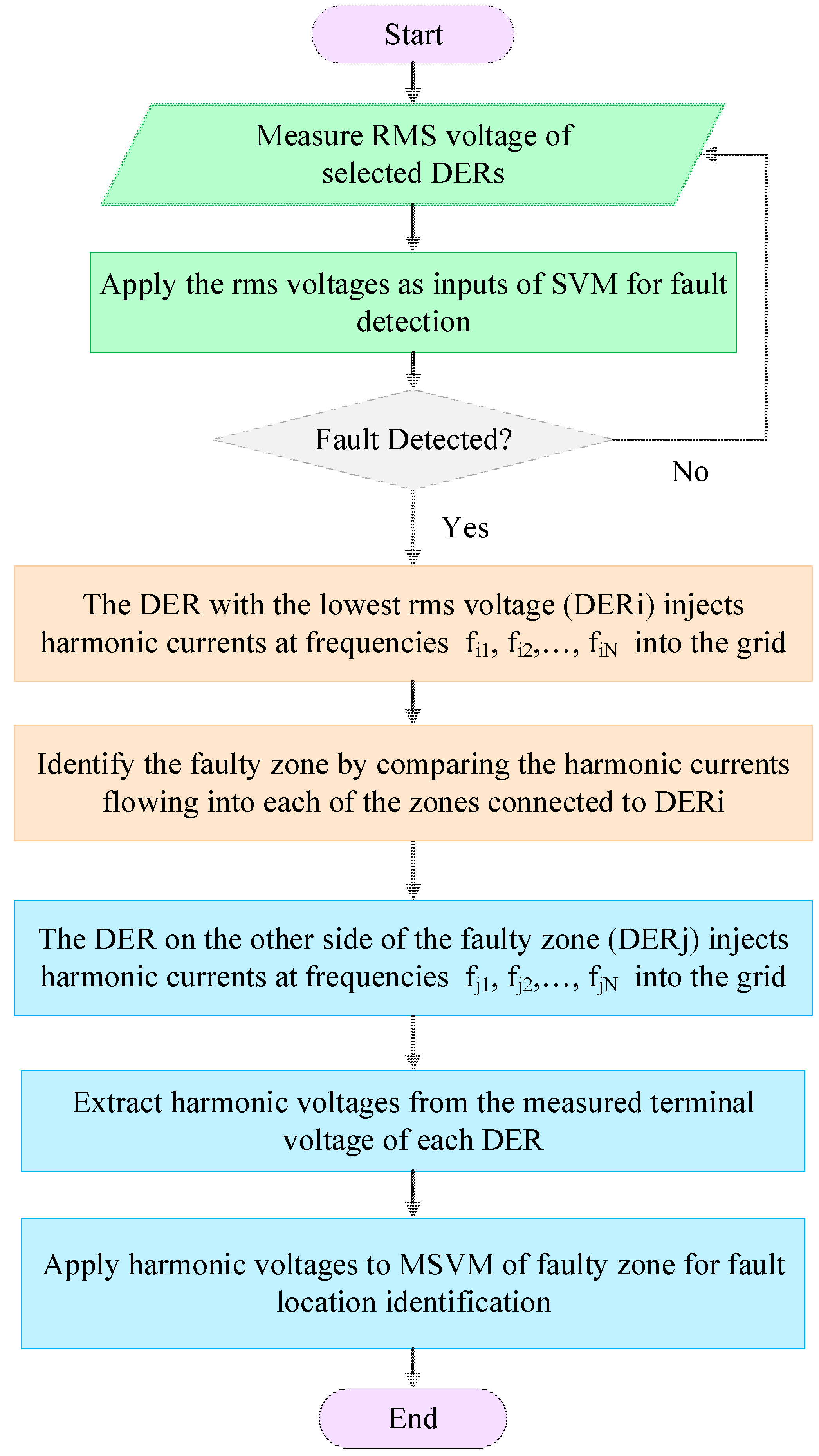
Figure 1 illustrates the proposed protection algorithm. The main stages of the algorithm are fault detection, identification of faulty zone, and finding the fault location. In the first step, the rms voltages of selected DERs are measured and a two-class SVM is applied. For each pair of DERs, a two-class SVM is employed, with class 1 referring to normal operation and class 2 referring to fault condition. As the voltage is very close to the rated value during the normal operation, but experiences a drastic drop during fault, the fault detector SVM offers high precision.

The fault location is detected in two steps: identification of the faulty zone detection of the faulty line. The MG is divided into a number of zones, each of which comprises a number of lines. The DER that is electrically closest to the fault experiences the lowest voltage level. This DER, which is denoted as DERi, injects interharmonic currents into the grid. The interharmonic currents passing through each of the zones connected to DERi are measured. The zone with highest interharmonic current is selected as the faulty zone.

Once the faulty zone is detected, the location of the fault within that zone is identified using a multi-class SVM (MSVM). To that end, the DER on the other side of the faulty zone (DERj) also injects interharmonic currents into the grid. It is worth emphasizing that each DER injects interharmonic currents with distinctive frequencies, which are not an integer multiple of the fundamental grid frequency. Accordingly, DERi and DERj inject interharmonic currents at frequencies {f_i1, f_i2, f_i3, …, f_iN} and {f_j1, f_j2, f_j3, …, f_jN}, respectively. They give rise to interharmonic voltages with the same frequencies at the terminal of DERi and DERj. After extraction of the interharmonic voltages, they are used as the inputs of the MVSM classifier, which determines the faulty line.

It is worth highlighting that harmonic currents and voltages are considered as power quality phenomena, which should be alleviated in normal operating conditions. Long-term presence of harmonic voltages and currents can have a detrimental impact on power system equipment and sensitive loads. To avoid this issue, the proposed scheme does not employ harmonic injection during normal operating conditions. Rather, harmonics are only injected into the grid after a fault is detected. The harmonic injection is only continued for a few milliseconds for the identification of fault location and stopped following fault isolation. So, the proposed scheme does not have any impact on the power quality during normal operating condition. Moreover, as fault occurrence is not frequent and the process of fault location identification is rapid, the duration of harmonic injection in comparison with system operation time is negligible.

3. Interharmonic Injection and Detection Schemes

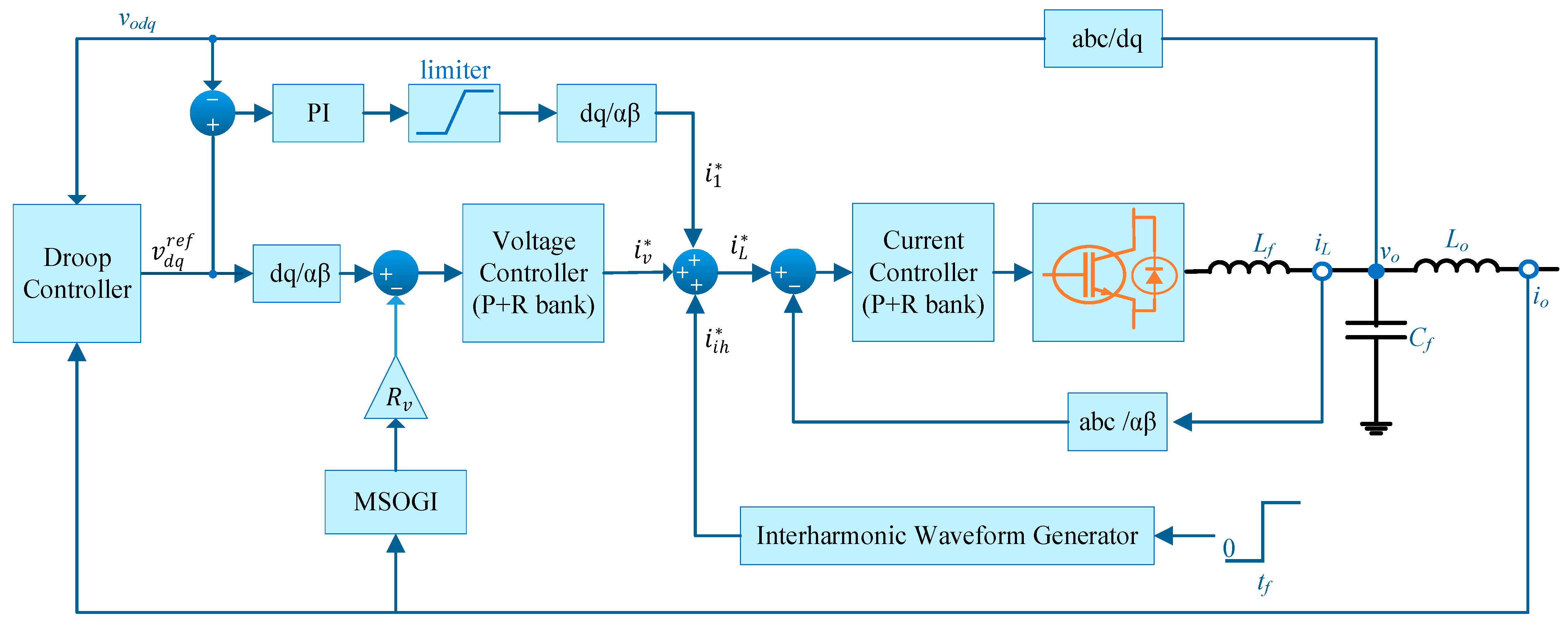
In order to realize the proposed interharmonic injection scheme while maintaining the DERs’ output currents below its maximum limit, the control structure of Figure 2 is proposed. The DERs’ reference output voltage (v_dqref) is calculated by the droop controller to satisfy the requirements of proportional sharing of load power among the DERs while regulating the MG voltage and frequency within an acceptable range [19]. This reference voltage is forwarded to the cascaded voltage and current control loops, which realize voltage reference tracking with zero steady-state error. Under normal operation conditions, the reference voltage is a balanced sinusoidal three-phase voltage. Therefore, zero steady-state tracking error can be ensured by adopting the PI controller in the dq frame or proportional resonant controller (P + R) in the αβ frame. Under fault conditions, however, several issues arise:

• The amplitude of the fundamental component of the output current must be limited to prevent overcurrent stress on the converter switches.
• Interharmonics at selected frequencies must be injected into the grid.
• Absorption of interharmonic currents generated by other DERs for fault detection must be prevented.

In order to realize the first objective, fundamental reference voltage tracking is realized by means of a proportional integral (PI) controller in the dq frame. The output of the PI controller is limited to obtain the fundamental reference current ($i_1^{*}$). It is worthwhile to note that realization of the limiting mechanism in dq frame (rather than αβ frame) is essential for preventing clipping, and hence distorting the fundamental current waveform.

During normal operation, the reference current does not reach its limit, hence the PI controller tracks the reference voltage with zero steady-state error. During fault condition, however, the limiter’s action causes a decrease in the reference current, and hence the output voltage drops below its set-point.

Upon detection of a fault (at t = t_f), interharmonics at frequencies {f_i1, f_i2, f_i3, …, f_in} are injected into the reference current of DERi. The “interharmonic waveform generator” generates α and β components of the interharmonic currents ($i_{ih}^{*}$) according to the following equations:

$$i_{ih,\alpha }^{*}={\displaystyle \sum _{n=1}^N{I}_n\cos \left(2\pi f_{in}t\right)}$$

(1)

$$i_{ih,\beta }^{*}={\displaystyle \sum _{n=1}^N{I}_n\cos \left(2\pi f_{in}t-\pi /2\right)}$$

(2)

The interharmonics injected by each DER must have distinctive frequencies. The combination of fundamental and interharmonic reference currents comprises a non-sinusoidal reference, which must be tracked by the current controller. To achieve zero steady-state tracking error, the P + R current controller employs a set of resonant filters with resonant frequencies equal to the frequency of the fundamental component and interharmonics. The transfer function of the current controller is

$$G_{cc}\left(s\right)=k_p+\frac{k_{r0}}{s^2+{\omega }_0}+{\displaystyle \sum _{n=1}^N\frac{k_{rn}}{s^2+{\omega }_{in}}}$$

(3)

where ω₀ is the fundamental angular frequency; ω_in is the angular frequency of the nth interharmonic injected by ith DER; and k_p, k_r0, and k_rn are the controller parameters.

The third requirement states that one DER must not absorb the interharmonic currents injected by another DER. In other words, from the perspective a DER, other DERs behave as high impedance loads, which do not have a considerable impact on the flow of interharmonic currents or voltages. To satisfy this objective, the unwanted interharmonics from other DERs are extracted by a multi-resonant second order generalized integrator (MSOGI). Then, a virtual resistance with high value is implemented for these extracted components.

The transfer function of a second order generalized integrator (SOGI) with resonant frequency ${\omega }^{\prime }$ is [20]

$$G_{SOGI}\left(s\right)=\frac{k{\omega }^{\prime }s}{s^2+k{\omega }^{\prime }s+{\left({\omega }^{\prime }\right)}^2}$$

(4)

SOGI works as a bandpass filter that has zero phase shift at the resonant frequency. The settling time of SOGI is approximately $10/k{\omega }^{\prime }$. So, by increasing k, the harmonic extraction process can be sped up. Nevertheless, an increase of k is also associated with increased bandwidth and lower attenuation of unwanted components. So, k must be selected by considering the trade-off between frequency selectivity and response time. By combining multiple SOGI blocks, a multi-resonant SOGI (MSOGI) block can be obtained. The MSOGI extracts each of the interharmonic currents based on the following equations [20]:

$$I_{kn,\alpha }\left(s\right)={G_{SOGI}(s)|}_{{\omega }^{\prime }={\omega }_{kn}}\left(I_{\alpha }\left(s\right)-{\displaystyle \sum _{i,n\ne k,n}{\displaystyle \sum I_{in,\alpha }\left(s\right)}}\right)$$

(5)

$$I_{kn,\beta }\left(s\right)={G_{SOGI}(s)|}_{{\omega }^{\prime }={\omega }_{kn}}\left(I_{\beta }\left(s\right)-{\displaystyle \sum _{i,n\ne k,n}{\displaystyle \sum I_{in,\beta }\left(s\right)}}\right)$$

(6)

where I_α, I_β, I_kn,α, and I_kn,β denote the α, β components of the total current and the interharmonic current at frequency ω_in, respectively. By subtracting the total current from the sum of extracted interharmonic currents (except the component at frequency ω_kn), MSOGI enables achieving high accuracy in terms of harmonic extraction. The extracted current is then multiplied by a virtual resistance (R_v) to obtain a voltage drop, which is in turn subtracted from the DERs’ reference voltage. The resulting voltage is then applied to the interharmonic voltage controller, which has the following transfer function:

$$G_{vc.PR}\left(s\right)={k^{\prime }}_p+{\displaystyle \sum _{i=1}^M{\displaystyle \sum _{n=1}^N\frac{{k^{\prime }}_{r,in}}{s^2+{\omega }_{in}}}}$$

(7)

where k’_p and k’_rn are the controller parameters. Equation (7) realizes a P + R bank with resonance frequencies equal to the corresponding interharmonic frequencies.

The injected interharmonic currents give rise to interharmonic voltages, which are sensed at the terminals of DERi and DERj. The α, β components of each voltage interharmonic are then extracted from the measurement results using MSOGI (see Equations (5) and (6)). Then, the amplitude the interharmonic voltage is obtained from the α, β components as follows:

$${\widehat{v}}_{kn}=\sqrt{v_{kn,\alpha }^2+v_{kn,\beta }^2}$$

(8)

The extracted amplitudes are used by the MSVM algorithm to identify the faulty line.

4. Results and Discussion

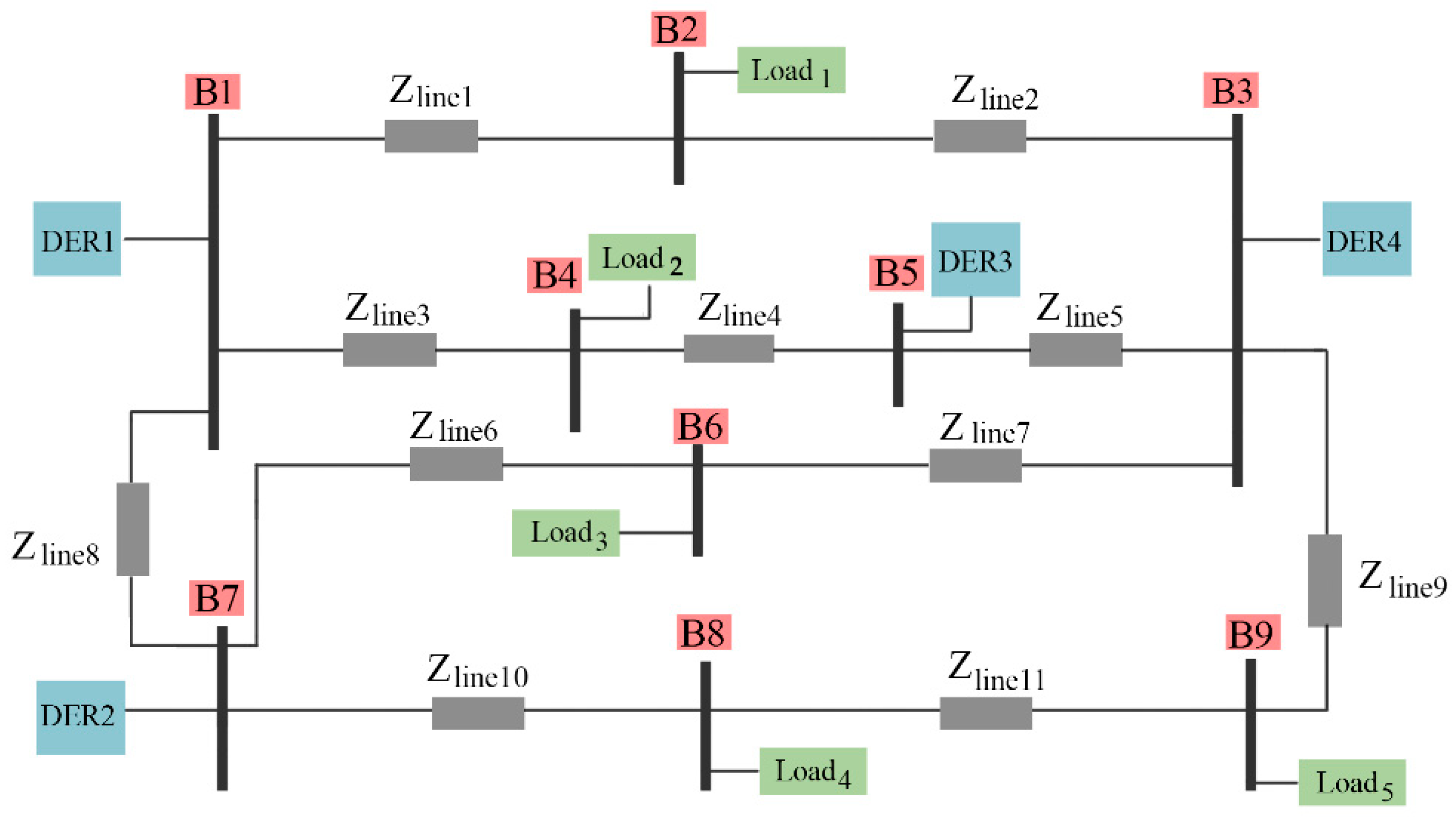
In order to demonstrate the efficacy of the proposed algorithm, it has been applied to the test MG of Figure 3. The test MG is comprised of four 3 kVA DERs connected to a meshed low voltage network. The specifications of the test MG are listed in

Table 1. Specifications of the test microgrid (MG).

Parameters	Symbol	Value
Rated voltage	Vrated	380 V
Rated frequency	f	50 Hz
Filter capacitance	C	25 μF
Filter inductance	L	1.8 mH
Output inductance	L0	1.8 mH
Constant active power load	PL1	1500 W
Constant active power load	PL3, PL4	1000 W
Constant resistive load	RL2, RL5	70.53 Ω
Line resistance	ZL1, ZL3, ZL4, ZL5, ZL6, ZL7 ZL8, ZL10, ZL11	1 + j0.43 Ω
Line resistance	ZL2, ZL9	2 + j0.86 Ω

. The MG has a rated voltage of 380 V and rated frequency of 50 Hz. The line impedances have a high R/X ratio, which is in accordance with the physical nature of distribution systems. The meshed topology of the network and the distributed nature of the sources cause the flow of fault current from various paths, which means that the detection of fault location is a challenging problem.

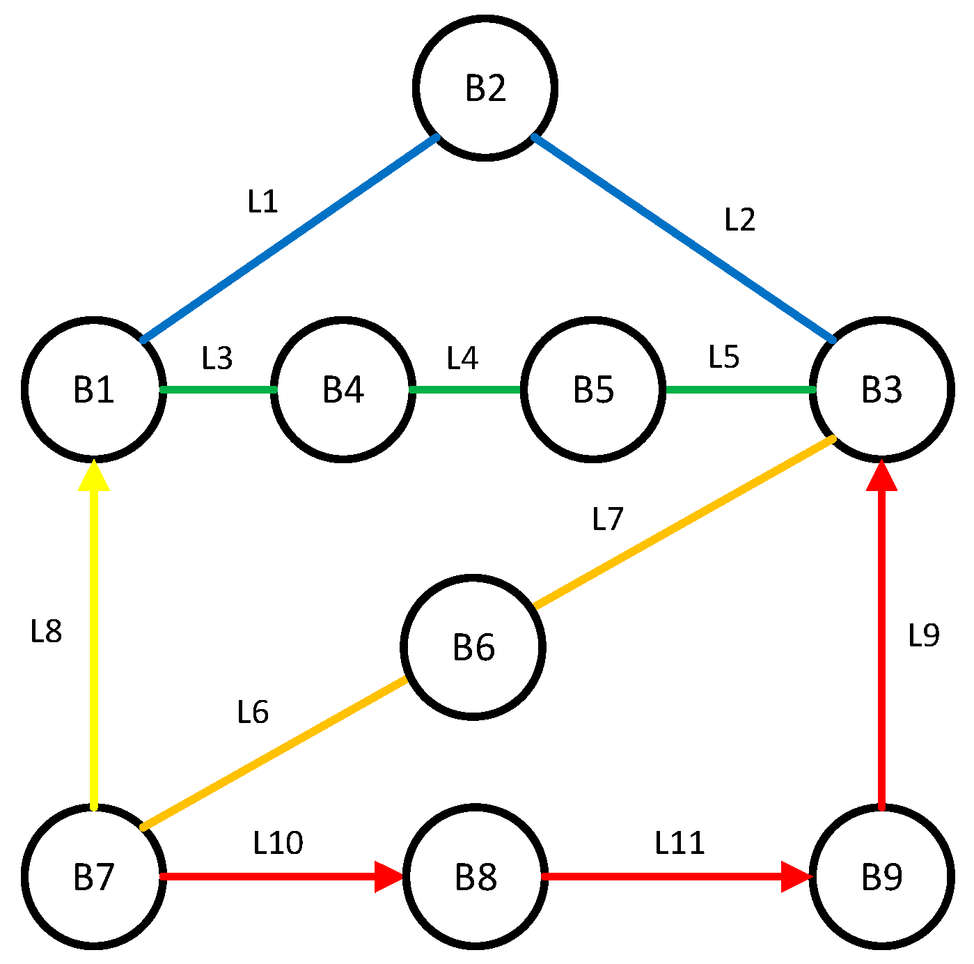
Figure 4 shows the protection zones of the test MG. Here, the network is represented by a graph, in which the nodes and edges express bus-bars and lines, respectively. The proposed algorithm does not require the contribution of all DERs. Considering the topology of the test MG, the DERs 1, 2, and 4, each of which has several lines connected to its terminal, are selected for realizing the algorithm. DERs 1, 2, and 4 are at nodes B1, B7, and B3, respectively. The collection of edges that lie across the path connecting each pair of these nodes are assigned as a protection zone. Each protection zone is shown with a specific color. The edges included in each of the zones are as follows: G_zone1 = {L1,L2}, G_zone2 = {L3,L4,L5}, G_zone3 = {L8}, G_zone4 = {L6,L7}, G_zone5 = {L9,L10,L11}. To identify the faulty zone, the DER that is electrically closest to the fault (DER with lowest rms voltage) injects interharmonic currents into the network and the currents flowing through each of the protection zones connected to that DER’s node are measured. The zone with the highest current is the faulty zone.

Although the algorithm can be implemented using a single interharmonic for each DER, the precision of the fault location can be improved by using multiple interharmonics. To demonstrate the attainable improvement, the test results for single interharmonic and triple interharmonics injection are presented. In both cases, the frequency of the injected interharmonics are selected as f = 50n + 25 (n = 4, 5, …,12). The maximum frequency of the injected current is 625 Hz, which is within the bandwidth of the inner loop’s closed loop transfer function. So, the inner loop is capable of tracking the reference current.

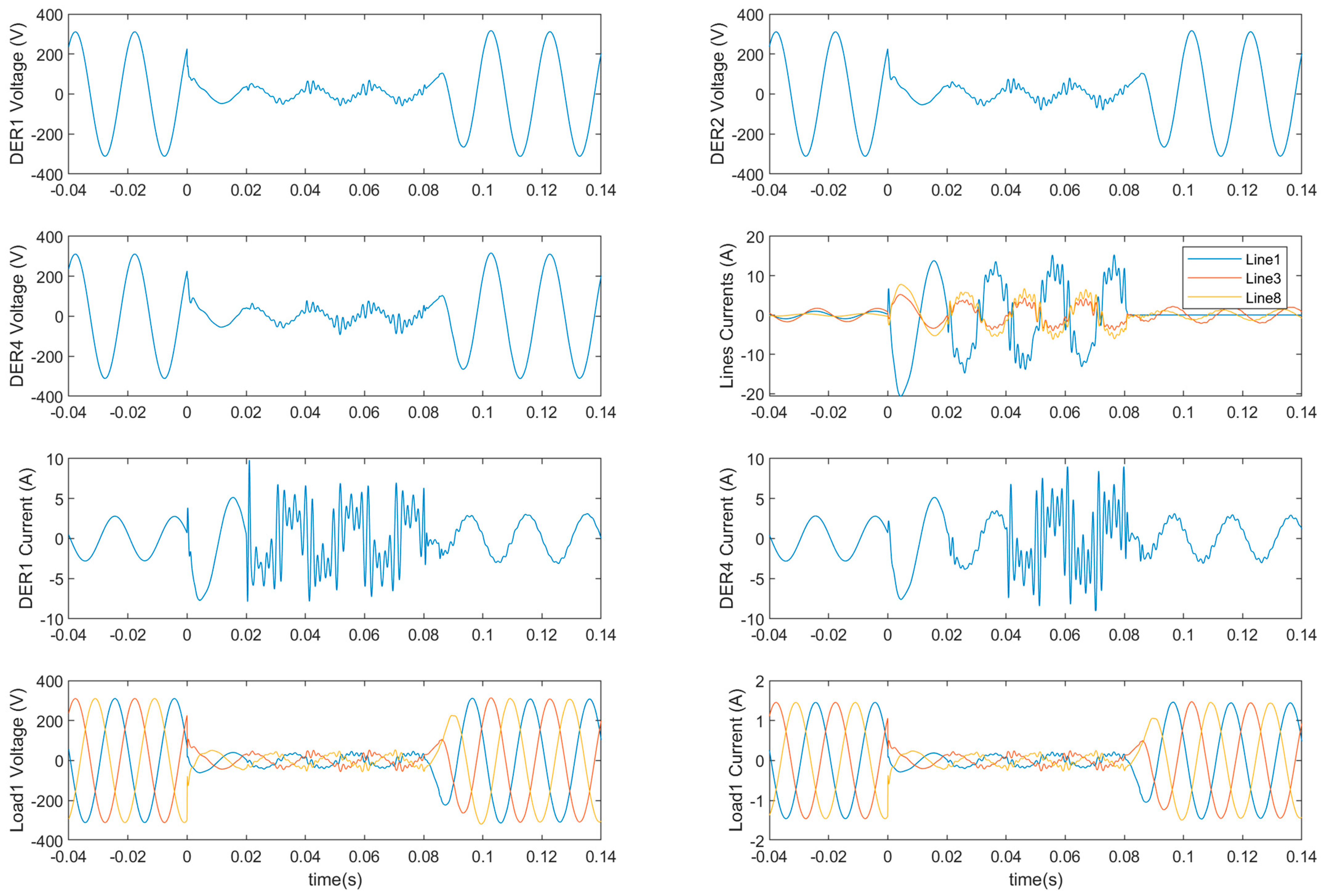
The simulation results for a three-phase short circuit fault in line 1 are shown in Figure 5. Prior to t = 0, the system is in normal operation condition with 50% loading. During this interval, the DER voltages are close to the rated voltage (peak voltage = 220√2) and the MG load is equally shared among the DERs. At t = 0 s, a short circuit fault with impedance of 1 Ω occurs in line 1. As a result, the voltages of each of the DERs’ current control loop decrease such that the current does not exceed the maximum value. The DER rms voltages are calculated and transferred to the fault detection SVMs. As the rms voltage calculation has a delay of one power cycle (0.02 s), the fault is detected by SVM at 0.02 s. It is seen that the voltage of DER1 drops to a lower value than the other DERs. This is a direct result of the lower electrical distance between the fault and DER1. Therefore, DER1 starts injecting interharmonics at frequencies of 325 Hz, 425 Hz, and 525 Hz. Then, the algorithm detects the faulty zone by comparing the harmonic currents of the three lines connected to DER1 (line 1, 3, and 8). Based on the fact that the harmonic current of line 1 is higher than the other two, zone 1 is detected as the faulty zone. In the next step, at time t = 0.04 s, DER4, which is on the other side of the faulty zone, injects interharmonics at frequencies of 375 Hz, 475 Hz, and 575 Hz. The injected interharmonic currents give rise to interharmonic voltages at the DER terminals, which are extracted by SOGI filters. The magnitudes of the 325 Hz, 425 Hz, and 525 Hz components at DER1 and 375 Hz, 475 Hz, and 575 Hz components at DER4 terminal comprise a set of six features for the MSVM of zone 1. Using these features, the MSVM classifier determines the faulty line. Consequently, the fault is cleared by disconnecting line 1 at t = 0.08 s.

To train the SVM classifiers, extensive simulations are conducted for normal and fault conditions. In normal operation conditions, the load is varied from 20% to 100% of the base value. In fault condition simulations, three phase short circuit faults with R_f varying in the range 0.5 Ω to 6 Ω are applied at different locations of the network. The maximum fault resistance (6 Ω) is the resistance that could raise the fault current to 200% of the rated value if the DER current limiting mechanism was not employed. The fault locations span over all of the lines with increments of 10% of each line’s length. Furthermore, load variations are considered in the fault condition simulations. The simulation results comprise a dataset, which is then randomly divided to training and test datasets. During the training process, an optimization problem is solved to obtain the classifier parameters such that the risk of misclassification is minimized (please see Appendix A for more details).

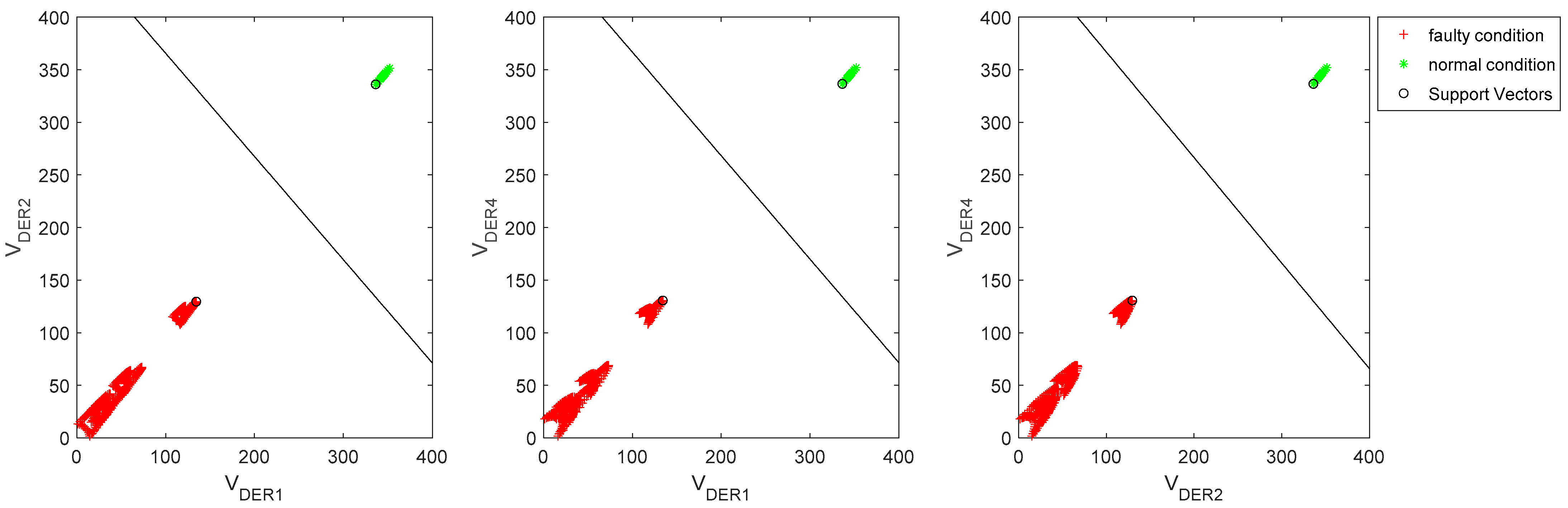
The first stage of the algorithm is fault detection. In this stage, the measured rms voltages of the DERs are applied to fault detector SVMs. Figure 6 shows the fault/normal condition classification results. It is observed that the rms voltages of fault and normal conditions, which are expressed by red and green color, respectively, are separable. This is caused by the fact that, upon inception of a fault, the current limiting mechanism of DERs causes a considerable decrease in the voltage, which drives the voltage out of the normal operating range. As a result, the fault and normal operation scenarios are completely discriminable by SVM classifiers.

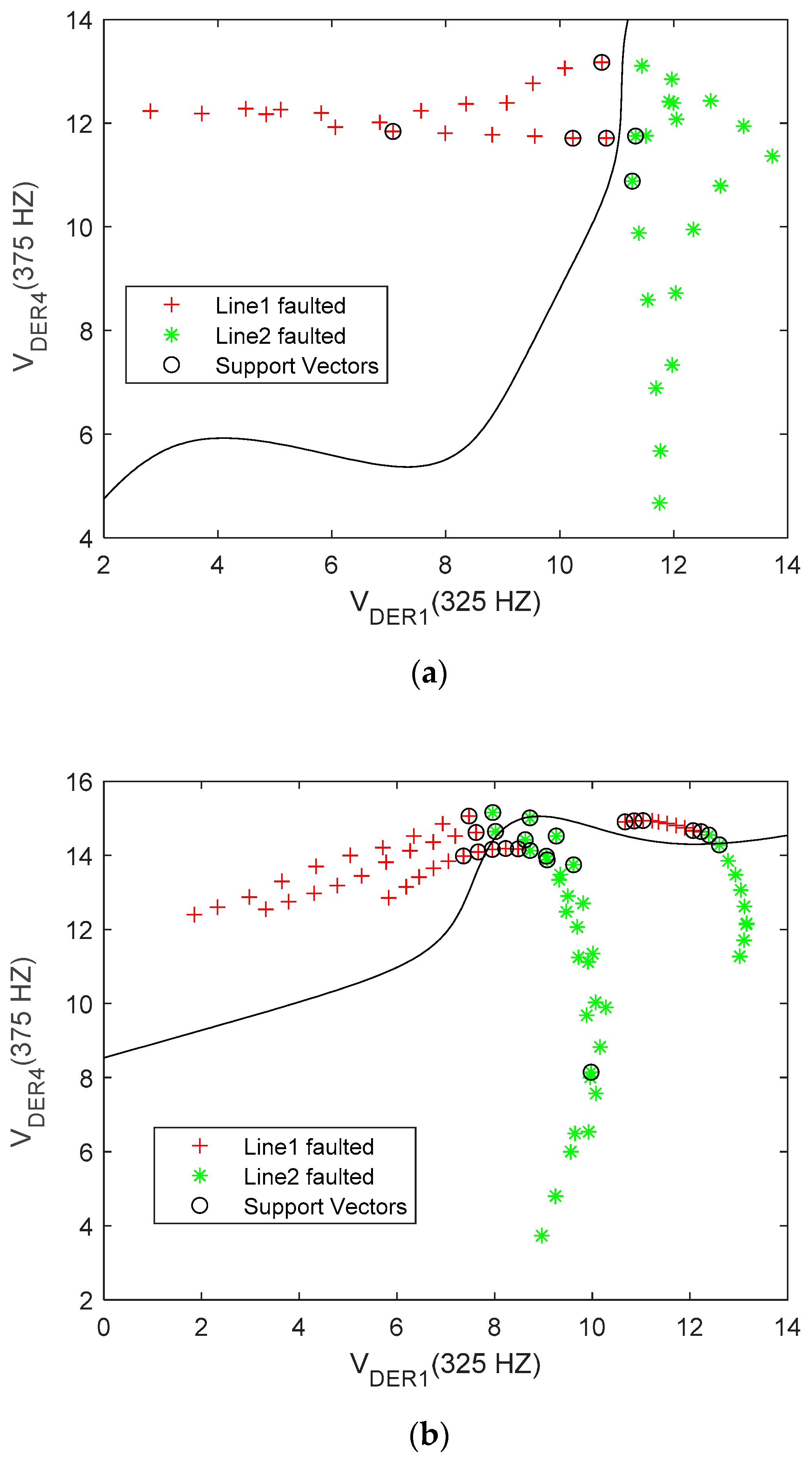
Following detection of fault, the faulty zone is identified. Once the faulty zone is identified, the second DER on the edge of the faulty zone also injects interharmonics into the MG. The resulting voltage interharmonics are measured by each of the DERs. These measurements comprise the features for MSVM, which identifies the faulty line. Consider the case in which a fault occurs in zone 1 (lines L1, L2) and assume that each of DERs 1 and 4 (which lie on sides of zone 1) inject a single interharmonic to identify the faulty line. Figure 7a shows the MSVM classifier for the specific case in which the MG load is at 100% and the R_f is 0.5 Ω. It is observed that the points corresponding with faults on each line are separable in this case. Therefore, the classifier is able to correctly identify the faulty line in all of the scenarios. However, such a good performance is not attainable in general, where the load and R_f vary. Figure 7b illustrates the SVM classifier that is trained by the entire dataset, comprising different values of R_f (0.5 Ω to 6 Ω) and loading (20% to 100%). Naturally, the classifier adapts itself to provide the optimum performance. However, as the points belonging to different classes are intertwined in this case, multiple cases of misclassification occur. Therefore, the single interharmonic scheme does not offer an acceptable accuracy in practice.

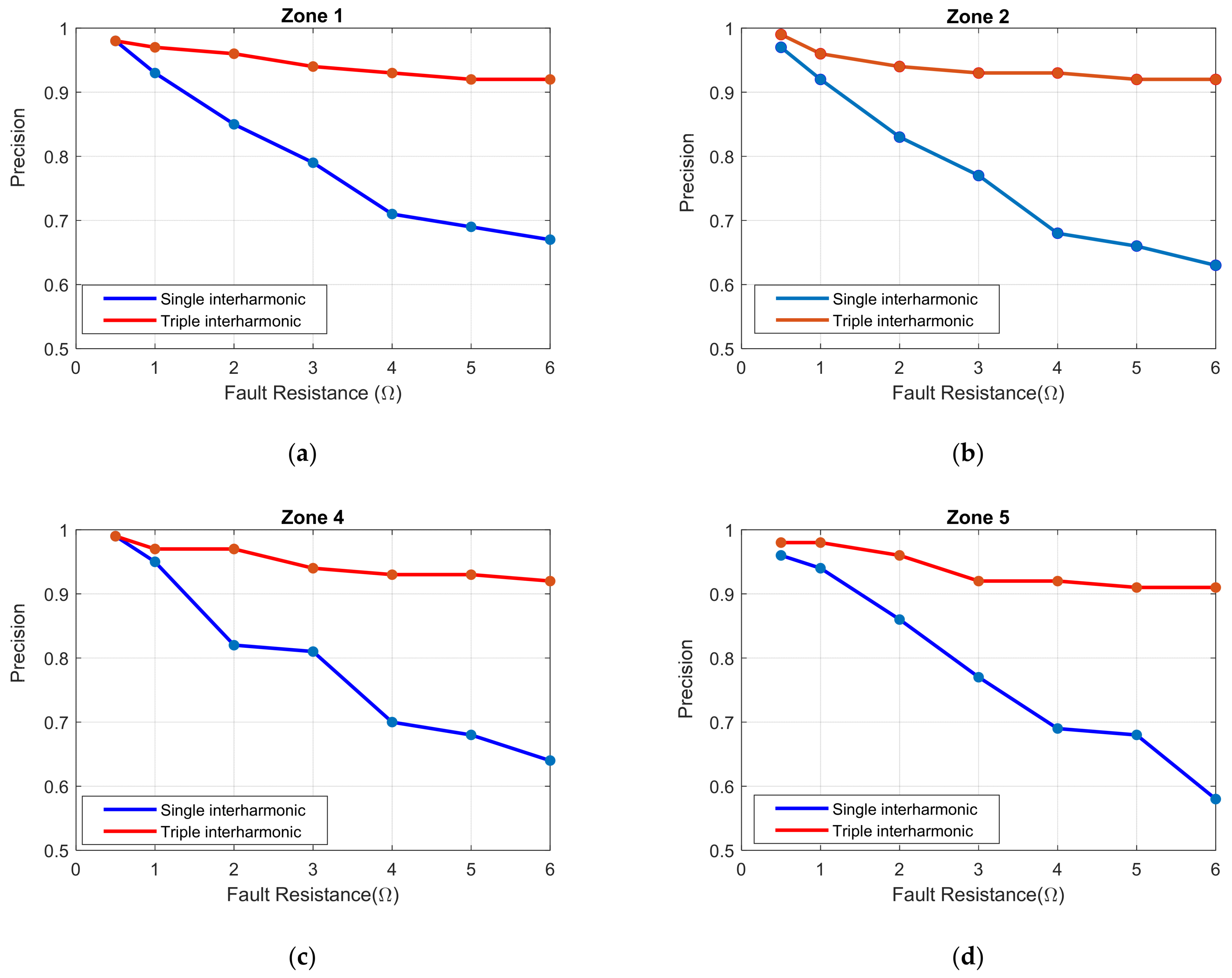
In order to enhance the accuracy of the MSVM classifier, a triple interharmonic injection scheme is proposed in this paper. In this scheme, each of the DERs on the sides of the faulty zone inject three interharmonics instead of one. In total, six current interharmonics are injected and six voltage interharmonics are measured. So, the number of features is increased from two to six in this case. So, the classifier is a hyperplane in 6D space, which is not possible to illustrate graphically. To demonstrate the enhancement obtained by the proposed scheme, its precision is compared with the single interharmonic injection scheme. Figure 8 shows the precision of the two schemes for faults occurring in each of the protection zones versus maximum value of the R_f. Figure 8a shows the precision for the case of a fault occuring in zone 1 (lines 1 or 2). It is observed that, while both schemes offer a high precision at R_f = 0.5 Ω, the precision of the single interharmonic scheme quickly drops with the increase of R_f. In contrary, the triple interharmonic scheme offers a high precision (>92%) over the entire range of R_f variations. Similar results are obtained for faults in other protection zones. It is seen from Figure 8d that, in the worst case scenario, i.e., fault with impedance of 6 Ω in zone 5, the triple interharmonic scheme offers an efficiency enhancement of 33%. Such precision enhancement is caused by two main reasons. Firstly, the triple interharmonic scheme increases the number of extracted features, which in turn enhances the MSVM’s precision. Secondly, in contrast with the line impedance, which comprises both inductive and resistive components, the fault impedance is mostly resistive. So, unlike the line impedance, the fault impedance is not frequency dependent. By processing three frequency components, the MSVM is able to cancel out the effect of fault impedance on the classification outcome.

5. Conclusions

The limited current capacity of DERs and existence of multiple current fault paths make the detection of fault location in MGs a challenging problem. To solve this problem, a machine learning-based algorithm is presented in this paper. In order to detect the occurrence of fault, the rms voltages of DERs are used as features for fault detector SVM classifiers. A fault condition is detected by comparing the voltage level of each pair of DERs with the fault detection line specified by the SVM. Once a fault is detected, the location of the fault, i.e., the faulty line, is identified using the harmonic injection method. To that end, each of the DERs inject interharmonic currents at one or three distinctive frequencies. The harmonic voltages are then extracted and used as features of an MSVM classifier. Using the voting algorithm, the classifier detects the faulty line. The accuracy of the MSVM classifier depends on the fault impedance and is also affected by load variations. With a zero fault impedance, the harmonic voltage is mainly dependent on the line impedance and fault location, hence the fault location is easily detectable. However, nonzero fault impedances and load uncertainties cause unwanted changes in the harmonic voltage, which can cause misclassification. In the case of a single interharmonic injection scheme, the precision of the MSVM considerably degrades with the increase of fault impedance. However, the triple interharmonic scheme offers highly accurate results for both low and high fault impedances. Such an enhancement is caused by the increased number of extracted features and different frequency response of line and fault impedances. The proposed scheme is tested on a meshed MG. Extensive simulation studies have been conducted to generate a comprehensive dataset, which encompasses fault location and impedance variations as well as load changes. The dataset is divided into training and test subsets, the former of which is used to train SVM and MSVM classifiers. The test results show that the triple interharmonic scheme offers a significantly higher precision compared with the single interharmonic strategy.