Ensuring Reliable Operation of Electricity Grid by Placement of FACTS Devices for Developing Countries

Abstract

Flexible AC Transmission Systems (FACTS) are essential devices used for the efficient performance of modern power systems and many developing countries lack these devices. Due to the non-existence of these advanced technologies, the national grid remains weak and vulnerable to power stability issues that can jeopardize system stability. This study proposes novel research to solve issues of an evolving national grid through the installation of FACTS devices. FACTS devices play a crucial role in minimizing active power losses while managing reactive power flows to keep the voltages within their respective limits. Due to the high costs of FACTS, optimization must be done to discover optimal locations as well as ratings of these devices. However, due to the nonlinearity, it is a challenging task to find the optimal locations and appropriate sizes of these devices. Shunt VARs Compensators (SVCs) and Thyristor-Controlled Series Compensators (TCSCs) are the two FACTS devices considered for the study. Optimal locations for SVCs and TCSCs are determined by Voltage Collapse Proximity Index (VCPI) and Line Stability Index ($L_{\mathit{mn}}$), respectively. Particle Swarm Optimization (PSO) is employed to find the ideal rating for FACTS devices to minimize the system operating cost (cost due to active power loss and capital cost of FACTS devices). This technique is applied to IEEE (14 and 30) bus systems. Moreover, reliable operation of the electricity grid through the placement of FACTS for developing countries has also been analysed; Pakistan being a developing country has been selected as a case study. The planning problem has been solved for the present as well as for the forecasted power system. Consequently, in the current national network, 6.21% and 6.71% reduction in active and reactive power losses have been observed, respectively. Moreover, voltage profiles have been improved significantly. A detailed financial analysis covering the calculation of Operation Cost (OC) of the national grid before and after the placement of FACTS devices is carried out.

1. Introduction

Despite the fact several developing countries have taken steps in the past to improve the electricity access for their deprived communities, most of them still lag far behind developed countries. Statistics show the electricity deprived population of the world sums up to 1.1 billion [1]. When analyzed geographically, Africa leads the list with about 62.5% (609 million) of the total population living without electricity. 20% of the total South Asian population (343 million), 3.5% of East Asia and Pacific population, 3% of the population in Latin America and 3% population of the Middle East and North Africa still lack access to electricity [2].

Multiple opportunities are available to improve the access to electricity in these deprived communities, such as focusing on more generation, improving energy efficiency, introducing demand-side management, and reduction in technical and non-technical losses. Moreover, it is pertinent to note that electricity saved is worth more than electricity generated [3]. After considering transmission and distribution (T&D) line losses, one kWh saved at the buyer end is 10% more beneficial than a unit saved at the generation [4]. However, in developing countries, T&D losses are usually around 20% of the total real power flow [5]. Therefore, it is more sustainable to focus on the reduction of power losses. Moreover, due to the rapid increase in power demand and integration of distributed energy resources, transmission lines usually operate close to their maximum loading points, thus causing power quality issues. These issues ultimately decrease the power transfer capability of the lines [6]. T&D losses is one of the major contributing factor of circular debt [7]. In general, financial issues of the power sector of a developing country have a devastating effect on its economy [8]. The focus of this research is to provide a techno-economical approach for the improvement of the existing transmission and distribution infrastructure of the developing countries. Pakistan being a typical developing country has been selected as a case study.

Pakistan has faced a severe energy crisis in recent years at a considerable cost to its economy. The power supply shortfall varied from about 5000 MW to 7000 MW during 2012–2015 [9]. The electricity supply of the country in 2019 was around 24,000 MW, whereas the demand was about 25,000 MW [10]. Furthermore, electricity demand is growing 10% annually, whereas the supply is increasing by 7%, thus leading to a gradual increase in the demand-supply gap [11]. This energy shortage started in 2006–2007 and kept on increasing till 2018. Insufficient generation capacity, obsolete power plants, circular debt, and inadequate transmission systems are some of the reasons for the severe energy crisis [12]. Circular debt has increased to 1.2 trillion PKR (Pak Rupees) in the last five years [13].

Literature reveals that electro-mechanical devices have been employed in the past to provide reactive power support and to improve real power flow [14]. However, these devices are inefficient and non-flexible to the changing conditions. Due to numerous drawbacks of electro-mechanical devices, all the developed countries have already shifted to modern controllers such as Flexible AC Transmission Systems (FACTS). The concept of FACTS was first introduced in 1999 by Hingorani et al. [15]. FACTS devices can enhance the overall Available Transfer Capacity (ATC) of the power system by controlling the current, voltage, and impedance of transmission lines and buses [16,17]. FACTS devices are mainly categorized into First, Second, and Third Generations. Shunt VARs Compensators (SVCs) and Thyristor-Controlled Series Compensators (TCSCs) belong to First Generation FACTS controllers, Static Series Compensator (STAT-COM) and Static Synchronous Series Compensator (SSSC) belong to Second Generation Controllers and Unified Power Flow Compensator (UPFC) and Inter-Line Power Flow Controllers (IPFC) belong to Third Generation Controllers [18]. Further details about the types of FACTS devices and their applications can be seen in [19]. Main objective of the study is to decrease real power losses and to improve the voltage profile of the electrical transmission system. It can be best achieved through TCSC and SVC [20]. TCSC can control line reactance’s thus providing series compensation, similarly, SVC can either inject or absorb reactive power to/from the system; hence can provide shunt compensation very effectively [21]. TCSC and SVC are mainly used to decrease real power losses and to improve the voltage profile of the electrical transmission system [22]. On the other hand, UPFCs can also control all the parameters (voltage, reactance, and angle). However, since UPFCs are more costly as compared to TCSC and SVC, installing UPFCs for this purpose will not be economically beneficial [19,23]. SVC requires less installation costs as compared to UPFC, hence SVC installation is the most appropriate choice for voltage stability [24]. Similarly, TCSC is more reliable as compared to STAT-COM for long-distance transmission lines [25]. When SVCs are compared to STAT-COM, STAT-COM gives efficient results at a higher cost [26]. Furthermore, the effectiveness of SVC and TCSC to decrease real power losses and to improve voltage profile have been discussed in the literature [27,28].

Optimum placement and sizing (OPS) of FACTS is very critical due to the high capital cost of these devices. In literature, various techniques for OPS of FACTS devices have been studied for standard IEEE systems. Basnal et al. discussed the OPS of FACTS devices to control reactive power using GA in [29]. In [30], authors have proposed a novel method to find out optimum locations of different types of FACTS devices based on bus and line voltage stability indices. Mixed Integer Linear Programming (MILP) for optimum placement of FACTS controllers has been proposed by Sharma in [31]. In [15], Biogeography Optimization (BO), Improved Weight PSO (IWPSO), and PSO have been applied to discover the optimal location of SVCs and ultimately reduce the power losses and voltage deviations. In [32], the application of PSO has been discussed for the optimal placement of FACTS to decrease the total system installation cost and to increase system load-ability. Power system stability has been improved using various FACTS devices in [33]. In [16], Whale Optimization Algorithm (WOA) has been applied for optimal placement of SVC and TCSC to achieve a reduction in total system operating cost. In [34], WOA has been used on multiple types of FACTS devices, and results are compared with existing metaheuristic optimization techniques. WOA showed considerable improvement in results as compared to others.

In [35], the placement of multiple SVC on the Nigerian grid system for steady-state operational enhancement is discussed. A Mixed-integer programming problem is used for placement of SVCs on 41 bus Nigerian national grid system. Contingency analysis in presence of an SVC controller is investigated for Sudan national grid [36]. After finding the locations for SVC placement, the mathematical models for the simulation of transmission line outages are carried out. In [37], the optimal placement of FACTs devices in the Iraqi National Super Grid System (INSGS) using a hybrid line stability index has been investigated. Only the optimal placement has been done on the national grid whereas a rating of the proposed FACTS devices has not been carried out. The literature study reveals PSO has been widely applied on standard systems to solve the planning problem of the FACTS devices. Few studies have been carried out for FACTS placement on the national grid, but no work has been reported in which PSO has been tested for the optimal sizing of TCSC and SVC on a national grid of any developing country.

The presented methodology is tested on IEEE-14 and 30 bus transmission systems [38]. After that, it is applied to the national power system of the developing country (Pakistan). As a result, a comprehensive planning model for reliable operation of the national grid for the developing country is presented. The main issues of improvement of voltage profile as well as reactive power compensation of practical national electrical transmission network are addressed through OPS of FACTS. It is observed that the active and reactive power losses of the national grid are seen to be reduced significantly. Moreover, significant financial savings have been observed as a result of FACTS placement. The payback period for the FACTS placement, both for the present and forecasted model is less than one year.

2. Methodology

SVC and TCSC are the two types of FACTS that are considered in this study. The main reason for selecting these devices is because of their higher cost to benefit ratio as compared to other FACTS devices [39]. TCSCs compensate for the inductive reactance of the transmission line by series connection and shunt connected SVCs are used for voltage control applications [40]. An SVC device can absorb or inject the required quantity of reactive power by controlling the firing angle of its thyristor [41]. Therefore, an SVC can help to regulate the bus voltage at a specified value despite load variations.

In the proposed method of placement and sizing of FACTS, sensitivity analysis has been carried out to determine weak buses and lines in the network. Weak lines and buses were identified using $L_{\mathit{mn}}$ and VCPI indices, respectively [16]. The main reason for selecting these indices for finding weak locations in the system is because they can be applied to a large power system with many buses and lines such as the national grid of any country. Moreover, as $L_{\mathit{mn}}$ index is a good pointer to determine weak transmission lines, the best locations for placement of TCSC can be obtained. Similarly, the VCPI index helps to determine buses prone to voltage collapse. All buses and lines are listed in order of decreasing indices so that the weakest buses and lines appear at the top of the list. Data clustering technique is applied to select clusters of weak buses and lines as the locations of SVCs and TCSCs. Since practical electrical networks constantly evolve due to the addition of more load, generation and transmission assets, it is agreed that some other lines and buses may turn out to be weaker, depending on the system under study. In such a case, the newly identified lines and buses can be considered for the placement of additional FACTS in the next phases.

After identifying the weakest locations in the system, PSO is applied to find optimal sizes of FACTS for the selected locations. It is pertinent to note that the optimal sizes of the FACTS device have been calculated with respect to each other and for simultaneous placement. Therefore, it is planned to simultaneously place all the finalized FACTS devices on the identified buses and lines.

2.1. Modelling of TCSC

Initially, TCSC was presented by Vithayatil to rapidly adjust the impedance of an electrical network [42]. TCSC is generally defined as a capacitive reactance compensator. The basic structure of TCSC consists of a capacitor, connected in shunt with thyristor-controlled reactors [28]. The number of such compensators can be placed in series to get desired operational characteristics.

By modifying the firing angle of the thyristor, TCSC can provide both inductive and capacitive compensations. The connection of TCSC to the transmission network and its characteristics with changing firing angle are discussed in detail in [19]. Active and reactive power flows in the presence of TCSC from bus p to bus q are presented in Equations (1) and (2).

$$P_{pq}= V_p^2{G}_{pq}-V_p{V}_q\left(G_{pq}cos{\delta }_{pq}+B_{pq}\sin {\delta }_{pq}\right)$$

(1)

$$Q_{pq} =-V_p^2\left(B_{pq}+B_{sh}\right)-V_p{V}_q\left(G_{pq}\sin {\delta }_{pq} - B_{pq}cos{\delta }_{pq}\right)$$

(2)

where $V_p$ represents the voltage of sending bus, $V_q$ is the receiving end bus voltage, $G_{pq}$ represents the line conductance, $B_{pq}$ is the susceptance of the line and ${\delta }_{pq}$ is the bus angle difference between the buses. Similarly, the power flow equations from the bus q to bus p can be written as:

$$P_{qp}= V_q^2{G}_{pq}-V_p{V}_q\left(G_{pq}cos{\delta }_{pq}-B_{pq}\sin {\delta }_{pq}\right)$$

(3)

$$Q_{qp}=-V_q^2\left(B_{pq}+B_{sh}\right)+V_p{V}_q \left(G_{pq}\sin {\delta }_{pq}+B_{pq}cos{\delta }_{pq}\right)$$

(4)

Equations (5) and (6) represent $G_{pq}$ and $B_{pq}$ of the transmission line, respectively:

$$G_{pq}= \frac{R}{R^2+{\left(X_{pq}-X_{Tcsc}\right)}^2}$$

(5)

$$B_{pq}= \frac{-X_{pq}-X_{Tcsc}}{R^2+{\left(X_{pq}-X_{Tcsc}\right)}^2}$$

(6)

where $G_{pq}$ represents the line conductance, $B_{pq}$ is the susceptance of the line R represents the resistance of line and X_pq is the reactance of line and X_TCSC is the reactance of TCSC.

2.2. Modelling of SVC

SVCs are used in high voltage transmission networks. These electrical devices are used to provide quick-response reactive power for enhancing power system stability, power factor correction, and voltage profile improvement. Primarily, SVCs are installed for two primary purposes, (i) To improve and regulate the voltage of the transmission network (transmission SVC) and (ii) To adjust the power quality of industrial loads (industrial SVC). In transmission networks, SVCs are generally used to enhance grid voltages. If the power system has a capacitive load, then SVC consumes “var” by utilizing thyristor-controlled reactors and regulates system voltages. However, if the power system load is inductive and the power factor is low, then SVC injects reactive power into the system for voltage profile and power factor improvement. The flexible nature of SVC mainly lies in inverse parallel and series-connected thyristors, which forms thyristor valves. The single line and control block diagram of typical SVC has been discussed in detail by F. Gandoman in [19].

SVCs are made of two or more fixed or switched banks of shunt reactors or capacitors, and one of the banks is thyristor switched. Typically, thyristor switched capacitors, mechanically switched reactors and capacitors, thyristor controlled reactors, and harmonic filters are used to make SVC. An SVC model is discussed in detail in [42]. The reactive support provided by SVC is mathematically shown as

$$Q_{svc}=V_n^{ }{}^2{B}_{svc}$$

(7)

where “$V_n$” is the voltage of bus at node “$n$”, and “$B$” represents the susceptance where SVC is connected.

2.3. Optimal Allocation of FACTS

FACTS devices take account of the transfer capacity of power transmission lines and regulate various parameters in the transmission network such as voltage, current, and impedance. However, the full benefit of any of these devices can be taken if they are utilized efficiently by optimal placement and appropriate sizing. Weak lines and buses are calculated in the system through $L_{\mathit{mn}}$ and VCPI, respectively, for optimal placement of FACTS which are discussed in the following sections.

2.3.1. Optimal Allocation of TCSC

TCSC is installed in a weak transmission line, which can be identified by the stability index ($L_{\mathit{mn}}$) of the transmission line. A transmission line with the value of $L_{\mathit{mn}}$ index closer to 1.0 is more unstable than a transmission line with the value of $L_{\mathit{mn}}$ index deviating further away from 1.0. $L_{\mathit{mn}}$ index can be calculated using Equation (8)

$$L_{\mathit{mn}}= \frac{4X{Q}_r}{{\left[V_s\sin \left(\theta -\delta \right)\right]}^2}$$

(8)

where “$X$” represents the line impedance and “$Q_r$” is reactive power demand of the receiving node of the transmission line, “$V_s”$ is the source voltage, “$\theta$” is the angle of impedance, and $“\delta ”$ is the difference in angle between buses.

2.3.2. Optimal Allocation of SVC

For optimal placements of SVCs, the VCPI index is used. The index helps to find out the unstable buses in a transmission system. VCPI index for all the buses are calculated, buses with index values close to 1.0 are considered weak. Therefore, such buses are the candidate locations for the placement of SVCs. VCPI works on the principle of maximum power transfer via line, and it is defined as:

$$VCPI= \frac{P}{P_{max}}$$

(9)

where

$$P=V_{r}Icos\varnothing$$

(10)

$$P_{max}=\frac{V_s^{2}cos\varnothing }{Z_s 4{cos}^2\left(\frac{\theta -\varnothing }{2}\right)}$$

(11)

where $V_s$ represents source voltage and $Z_s$ is impedance. $\theta$ is the impedance angle and $\varnothing$ is the angle difference between sending (“From” Bus) and receiving end bus (“To” Bus).

2.4. Optimal Sizing of FACTS

To decrease total system operation cost, PSO is used to calculate optimal sizes of TCSCs and SVCs for each selected location.

2.4.1. Mathematical Formulation

The main objective of finding the optimal rating of FACTS is to minimize both the costs due to active power loss and FACTS installation cost. The objective function is mathematically written in Equation (12). Ratings of FACTS devices are changed in each iteration by PSO; hence active power loss is calculated in every iteration, which is then multiplied by the cost of electrical energy. In Equation (13), “0.09$” is the per-unit cost of electrical energy [43], which is multiplied by total active power losses of the entire system (P_L) for the whole year (365 × 24). To minimize this value, active power losses are calculated in every iteration of PSO using the Newton Raphson power flow method, which is run in MATPOWER. The overall objective function is as follow

$$\min \left[C_{PL}+ C_{FACTS}\right]$$

(12)

where $C_{PL}$ is the cost associated with active power loss and calculated as follows

$$\mathrm{Minimize} O_1\left(x_1,x_2\right) P_{loss}= {{\displaystyle \sum }}_{k=1}^{n_{ }}\left[G_k\left(V_i^2+V_j^2-2V_i{V}_{j}cos{\delta }_{ij}\right)\right]\times (0.09 \$/\mathrm{kWh}) \times 365 \times 24$$

(13)

where $O_1=\left(x_1,x_2\right)$ is an active power loss function that needs to be minimized. $G_k$ is the conductance of line k. $V_i^{ }$ and $V_j^{ }$ are the voltage magnitude of sending and receiving buses ${\delta }_{ij}$ is the phase difference between ith and jth bus. Here $x_1$ is an array of dependent variables and $x_2$ is an array of control variables and can be defined as follows.

$$x_1 = \left[V_{L1}\dots V_{Ln} , Q_{G1}\dots Q_{Gn} , S_{L1}\dots S_{Ln}\right]$$

(14)

$$x_2 = \left[SV{C}_1\dots SV{C}_n , TCS{C}_1\dots TCS{C}_n \right]$$

(15)

$\left(V_{L1}\dots V_{Ln}\right)$ are voltages at load buses, $(Q_{G1}\dots Q_{Gn})$ are reactive power from all the generators, $(S_{L1}\dots S_{LN})$ are transmission line loading, $(SV{C}_1\dots SV{C}_n)$ are SVCs and $(TCS{C}_1\dots TCS{C}_n)$ are TCSCs. The respective limits of both these devices are defined in Equations (20) and (21).

Moreover, $C_{FACTS}$ is the cost of FACTS devices and are given by the quadratic equation as shown in Equations (17) and (18).

$$C_{FACTS} = C_{TCSC}+C_{SVC}$$

(16)

$$C_{TCSC}=0.0015t^2-0.7130t+153.75\left(\frac{\$}{\mathrm{kvar}}\right)$$

(17)

$$C_{SVC}=0.0003s^2-0.3051s+127.38(\frac{\$}{\mathrm{kvar}})$$

(18)

where $t$ and $s$ are the sizes of TCSC and SVC in kvar, respectively. The quadratic cost functions of TCSC and SVC are defined by ABB, as discussed in [34].

Equality Constraints that need to be satisfied are as follows:

$$P_{Gi}-P_{Di}-V_i{\displaystyle \sum }_{k=1}^n{V}_j\left[G_{ij}cos{\delta }_{ij}+B_{ij}\sin {\delta }_{ij}\right]=0$$

(19)

$$Q_{Gi}-Q_{Di}-V_i{\displaystyle \sum }_{k=1}^n{V}_j\left[G_{ij}cos{\delta }_{ij}+B_{ij}\sin {\delta }_{ij}\right]=0$$

(20)

where $P_{Gi}$,$P_{Di}$, $Q_{Gi}$, and $Q_{Di}$ are the active and reactive power generation and demand at bus i and j and the total numbers of buses are represented by n.

While the Inequality Constraints of the optimization problem are given below:

$$V_{min}\le V_j\le V_{max}$$

(21)

$$-0.8X_L\le X_{TCSC}\le 0.2X_L pu$$

(22)

$$-0.9\le B_{SVC}\le 0.9 pu$$

(23)

$V_{min}$ and $V_{max}$ represent the minimum and maximum allowable voltages. Equations (22) and (23) have been used to ensure that FACTS devices are within their respective permissible limits. Since the optimization problem is nonlinear, PSO is applied to find out the optimum solution.

2.4.2. Particle Swarm Optimization

PSO is a heuristic optimization technique based on the food searching behavior of a set of birds or fishes [44]. In this technique, each affiliate of the group alters its behavior based upon the behavior of the swarm. A set of elements is initialized by randomly placing each particle of the group in the search space and then updating their positions based on their fitness evaluation. The velocity of each particle is updated, and a new solution is achieved. The iterative process continues until the optimal solution is obtained.

PSO has been applied in the following way:

Step 1: PSO initialization

PSO is initialized by specifying the bus and transmission line data. Candidate locations for placement of FACTS devices that have already been obtained by $L_{\mathit{mn}}$ and VCPI indices are initialized as array particles. The total number of particles, starting inertial weights, and the maximum number of iterations are finalized. Moreover, constraints on the size of FACTS devices are defined in the search space. Velocities and particle sizes are initialized arbitrarily. Particles are nothing but sizes of SVCs and TCSCs.

Step 2: Fitness function Evaluation.

AC power flow is run in each iteration to find out active and reactive power losses. The objective function for every particle array is assessed by calling the objective function independently.

Step 3: $G_{best}$ and $P_{best}$ Evaluation

$P_{best}$ denotes personal best (minimum value of the objective function) of each array among all iterations. $G_{best}$ (global best) is the minimum value of the fitness function. $P_{best}$ and $G_{best}$ are updated in each iteration after comparison with the previous iteration values.

$$P_{best}{}_p^{i+1}=[\begin{array}{c}{X}_p^{i+1} f_p^{i+1}\le f_p^i\\ P_{best}{}_p^i f_p^{i+1}\ge f_p^i\end{array}$$

(24)

where $f_p^i$ is the particle fitness value at iteration “$i$”, and “$p$” specifies the particle. The formula used to update $G_{best}$ is,

$$G_{best}{}_p^{i+1}=[\begin{array}{c}{P}_{best}{}_p^{i+1} f_p^{i+1}\le f_p^i\\ G_{best}{}_p^i f_p^{i+1}\ge f_p^i\end{array}$$

(25)

Step 4: Update position and velocity

After updating the values of $P_{best}$ and $G_{best}$, particle velocity is updated to lead it towards the optimum position. Velocity is updated after every iteration as:

$$V_p^{i+1}=w\times v_p^i+c1\times ran{d}_1\times \left(P_{best}{}_p^i-s_p^i\right)+c2\times ran{d}_2\times \left(G_{best}{}_p^i-s_p^i\right)$$

(26)

where $“i”$ represents iteration number, $“w”$ is the inertial weight, $ran{d}_1$ and $ran{d}_2$ are random numbers in the range of [0, 1], $“c2”$ and $“c1”$ are acceleration coefficients ranging between [1, 2] and $“s”$ represents the particle position.$“w”$ is updated in every iteration using Equation (25).

$$w=w_{max} \frac{w_{max}-w_{min}}{Max Iterations}\times i$$

(27)

$$S_p^{i+1}= S_p^i+V_p^{i+1}$$

(28)

2.4.3. Flow Chart for Placement and Sizing of FACTS

The complete procedure of the placement and sizing of FACTS devices is presented as a flowchart in Figure 1.

The proposed method for placement and sizing of FACTS devices is more compact, flexible and easy to implement as compared to other methodologies present in the literature. For instance, in [40] researchers have used the Fast Voltage Stability Index (FVSI) for the placement of TCSCs, however, as reactive power changes its results can become inaccurate and sub-optimal. Similarly, the authors of [34] have constructed PV curves of all load busses. Buses with more voltage deviations are weak and consequently optimal locations for SVCs placement. However, in a meshed network, where there are several interconnected buses, it is almost impossible to construct PV curves of all load buses to identify weak buses. In [40], researchers have calculated sensitivity indices for placement of TCSCs and SVCs by partial differentiating reactive power balance equation for the control parameter of respective FACTS device. Although this technique can give accurate results, implementing it on an extensive meshed system is very difficult. Similarly, in [16,45] and [22] authors have considered locations carrying higher active and reactive power as the best locations for FACTS placement. However, just considering the flow of real and reactive power for the placement of FACTS will not give accurate results, and thus the solution may not be optimal. The selected indices i.e., VCPI and $L_{mn}$ are easy to implement, will give accurate results and can be applied to any system irrespective of the complexity of the power network.

3. Results and Discussion

The method is initially tested on IEEE-14 and 30 bus systems, then it is applied to the Pakistani grid. Results of the test systems and Pakistan Grid are explained below.

3.1. Test Case IEEE-14 and 30 Bus Systems

IEEE-14 and 30 bus systems considered are from MATPOWER [38]. Summary of power generating units, transmission lines, and load buses have been summarized in

Table 1. IEEE 14 and 30 Bus Systems.

S. No		IEEE-14 Bus System	IEEE-30 Bus System
1	Power Generating Units	5	6
2	Transmission Lines	20	41
3	Load Busses	9	20

.

To find the candidate locations for TCSC and SVC placements, weak lines and buses are identified using $L_{mn}$ and VCPI indices, respectively. Load flows are calculated using the Newton Raphson power flow method in MATPOWER to calculate these indices. $L_{mn}$ and VCPI indices are determined by using Equations (8) and (9) respectively. Results for $L_{mn}$ index for IEEE-14 Bus systems are shown in

Table 2. $L_{mn}$ index values of lines (IEEE-14 Bus System).

Line	Branch	${\mathit{L}}_{\mathit{m}\mathit{n}}$ at Maximum Loading Point	Rank
4–7	8	0.998	1st
4–9	9	0.993	2nd
7–9	15	0.97	3rd
10–11	18	0.89	4th
13–14	20	0.8	5th
4–5	7	0.78	6th
9–14	17	0.67	7th
12–13	19	0.629	8th
9–10	16	0.587	9th

.

Branches 8, 9, 15, and 18 are weak lines and thus they can serve as candidate locations for placement of TCSCs. Similarly, VCPI is calculated for all buses as shown in

Table 3. VCPI values of all load busses (IEEE-14 Bus System).

Load Bus No.	VCPI at Maximum Loading Point	Rank
14	1.0023	1st
4	1.0007	2nd
9	0.9704	3rd
5	0.9363	4th
11	0.906	5th
12	0.8904	6th
7	0.8687	7th
13	0.8355	8th
10	0.8173	9th

, and those buses which have a VCPI value close to 1 are considered weak and thus optimal locations for placement of SVC. Here buses 14, 4, 9, and 5 are weak buses.

After finding candidate locations for TCSC and SVC, PSO is utilized to find the optimal rating for these devices. The optimal rating of FACTS devices and their effect on power loss is shown in

Table 4. Optimal rating of FACTS and its effect of system power losses (IEEE-14 Bus System).

Type of FACTS	Location	Optimal Rating (p.u)	Power Loss without FACTS (p.u)	Power Loss with FACTS (p.u)	Power Loss Reduction (p.u)
TCSC	4–7	0.081
TCSC	4–9	0.079
TCSC	7–9	0.08
TCSC	10–11	0.077	0.1436	0.092	0.052
SVC	14	0.0453
SVC	4	0.468
SVC	9	0.249
SVC	5	0.0891

.

SVC can greatly improve the voltage of the whole power system because they can effectively control VAr in the system, as illustrated in Figure 2. The voltages before FACTS are scattered between 0.95 and 1.05 but mostly fall below 1 p.u. However, after the placement of SVC and TCSC voltage profile is almost stable above 1 p.u.

It can be observed from the above-mentioned figure that the solution with only 1 SVC (dark green line) improves the voltage of bus 14, but is not able to improve the voltages of the other buses (e.g., bus 4). Similarly, the solution with only 1 TCSC (purple line) shows a lot of variability in the voltages of buses 1 through 5. However, the proposed solution (light green line) is able to keep the voltage profiles of all the buses sufficiently stable. Similarly, the effect of FACTS placement in the IEEE-30 Bus system is shown in

Table 5. Optimal rating of FACTS and its effect on system power losses (IEEE-30 Bus System).

FACTS Type	Location Bus/Branch	Optimal Rating (p.u)	Total True Power Loss without FACTS (p.u)	Total True Power Loss with FACTS (p.u)	Total Reduction in True Power Loss (p.u)
TCSC	7	0.051
TCSC	15	0.039
TCSC	20	0.01
TCSC	28	0.067	0.1755	0.130	0.0425
SVC	30	0.017
SVC	29	0.5
SVC	26	0.38
SVC	25	0.11

.

Figure 3 shows that there is a significant enhancement in the overall voltage profile of the IEEE-30 bus system after adding FACTS devices. Hence by placing SVCs of optimal rating at the weakest locations can greatly enhance the overall voltage profile of the network.

3.2. Practical National Grid of Developing Country

The proposed method of optimal placement and sizing of FACTS devices is tested on standard IEEE systems and then applied on the national grid of a developing county (Pakistan). The electricity deficit for the year 2013 to 2017 for the electric grid has been summarized in Figure 4.

T&D losses in lines are one of the biggest problems in most developing countries. The losses include technical losses due to heating in lines and un-metered losses because of theft. In the Pakistan grid, the distribution losses in some Distribution Companies (DISCOs) are more than 30% [5]. With the addition of 10,000 MW generation capacity in the past few years, some improvement in energy deficit has been observed. However, transmission lines started operating at their maximum loading point due to severe overloading [46]. Figure 5 summarizes the total transmission and distribution losses for the Pakistan grid from years 2015 to 2020 [10].

Most of the developing countries lack adequate power system planning but the implementation of envisaged plans is even more challenging. For long term planning, it is crucial to model processes and components of generation, transmission, and distribution systems. There are various commercial software’s available for power system planning and analysis. In this research work [21], MATPOWER has been used to model and study the electrical network. The study has been implemented on current (for the year 2018) as well as forecasted national gird (Year 2025) of Pakistan. The research has been done in collaboration with the power system planning department of the National Transmission and Dispatch Company (NTDC). NTDC is responsible to manage the transmission backbone to link Power Generation Units with Load Centers spread all over the country. All the data used in the research has been shared by NTDC containing its real grid expansion plans.

Present national grid model consists of 3651 buses, 4147 overhead transmission lines, 277 generating buses, and 1930 load buses. The total active power loss in the present electric grid was 853 MW, whereas the reactive power loss was 9951 MVAr. Data of the national network is in per-unit, referred to as the base voltage of 500 kV and base power of 100 MVA. The T&D network of Pakistan includes six voltage levels: 500, 220, 132, 66, 33, and 11 kV, out of which high voltage transmission network (500 kV, 220 kV and 132 kV) are owned and operated by NTDC and remaining by the Distribution Companies (DISCOs). The number of buses at each voltage level in the network model 2018 and 2025 are listed in

Table 6. Buses Details of National Grid.

Sr. No	Bus Voltage (kV)	Number of Buses
		Present Model	Forecasted Model
1	500	26	53
2	220	86	192
3	132	1222	1994
4	66	153	233
5	33	16	114
6	11	2148	3094

.

According to the data used for simulations (i.e., data for peak load condition in summer 2018 and 2025), 277 GENCOs were connected to the NTDC transmission network in 2018 which is forecasted to be increased to 797 generating stations till the year 2025. These power plants are mainly thermal and hydropower plants, but nuclear, wind, and solar PV plants are also part of the energy mix of the country with minor contributions. The peak load in 2018 reached 21,483.6 MW on 11 July 2018 which is forecasted to rise to 42,000 MW by 2025. The peak demand was mainly driven by air-conditioning systems. In the anticipated national grid for the year 2025, predicted load is around 41,000 MW whereas generation is around 42,000 MW. The grid system model includes 6007 busses, 797 generator busses and 2961 load busses and 10,110 transmission lines. An overview of the electrical components of the Pakistan national grid used in this study is presented in

Table 7. Summary of National Grid for both current and forecasted network.

Sr. No	Description	National Grid
		Present Model	Forecasted Model
1	Total Number of Buses	3651	6007
2	Power Generating Units	277	797
3	Transmission Lines	4147	10,110
4	Load Busses	1930	2961
5	Total Generation Capacity	73,343.7 MW	20,405.90 MW
6	Generation (actual)	22,337.3 MW	42,434.4 MW
7	Load	21,483.6 MW	40,584.5 MW

.

AC load flow analysis is done using the Newton Raphson method and is carried out in MATPOWER. According to load flow results, the power system is weak and vulnerable and has very high active and reactive power losses. Thus, the system is in dire need of modern devices such as FACTS.

3.2.1. Finding Weak Lines Using $L_{\mathit{mn}}$ Index

Weak lines in the whole system are identified as optimal locations for TCSC’s placement. Therefore, starting with the cluster of the weakest lines in the first phase, FACTS can be placed on clusters with decreasing vulnerability in subsequent phases. From the results, a bunch of seven lines listed in

Table 8. Weakest cluster of transmission lines in presented and forecasted Grid.

Grid Model	From Bus (kV)–To Bus (kV)	${\mathit{L}}_{\mathit{mn}}$ Value	Rank
2018	Dadu (220)–Khuzdar (220)	0.859	1st
	D G Khan (500)–Guddu (500)	0.835	2nd
	Sarfaraz Nagar-I (220)–Okara-I (220)	0.832	3rd
	Sarfaraz Nagar-II (220)–Okara-II (220)	0.832	4th
	M. Garh (500)–Guddu (500)	0.805	5th
	Lalazar-I (220)–Maripur-I (220)	0.799	6th
	Lalazar-II (220)–Maripur-II (220)	0.799	7th
2025	Shahi Bagh (220)–Jamrud (220)	0.923	1st
	Tarbela (500)–Gatti (500)	0.882	2nd
	Dadu Khel (220)–Bannu (220)	0.874	3rd
	Sialkot (220)–Ghakkar-II (220)	0.847	4th
	Okara (220)–Yousafwall (220)	0.831	5th
	Sumundri (220)–Multan (220)	0.811	6th
	Nagshah (220)–M. Garh (220)	0.792	7th

were identified as the weakest lines and thus suggested as candidate locations for placement of TCSCs.

3.2.2. Finding Weak Buses Using VCPI Index

VCPI values for the national grid were calculated and the list of buses was sorted in order of descending VCPI values. A cluster of six most vulnerable buses with the highest values of VCPI, listed in

Table 9. VCPI values for present and forecasted Grid.

Grid Model	Bus Name	Base Voltage (kV)	VCPI Value	Rank
Current Model	Ludewala	220	0.963	1st
	Port Qasim	500	0.905	2nd
	Guddu	500	0.889	3rd
	Sarfaraz Nagar	220	0.807	4th
	Bandalan	220	0.758	5th
	Multan	220	0.738	6th
Forecasted Model	Quetta	220	0.999	1st
	Bannu	220	0.973	2nd
	Moro	500	0.963	3rd
	Muzaffar Garh	500	0.935	4th
	Okara	220	0.919	5th
	Gujrat	220	0.878	6th

, were selected for placement of SVC in the first phase.

Optimal locations of FACTS devices in the 2018 and 2025 model are marked on the country’s map, as shown in Figure 6. In 2018, the cluster of weak locations is in central and southern Punjab i.e., the buses and transmission lines in the areas of Guddu, Multan and Muzaffargarh. The problem has been well identified and tackled by the planning department of NTDC. In the network planned for 2025, the weak lines that appeared as weak lines for the year 2018 are now stable. Some industrial load hubs, planned under the China–Pakistan Economic Corridor (CPEC) program, turn out to be relatively weak links. For example, the load of special economic zones near Peshawar, Quetta and Faisalabad will turn nearby buses and lines into relatively stressed points in the national grid planned for 2025.

3.2.3. Optimal Rating of FACTS and Its Effect on National Grid Losses

After determining suitable locations of FACTS devices, the next task was to find out appropriate ratings for the selected devices. A heuristic-based optimization technique called PSO has been utilized to minimize the total Operating Cost (OC), including costs of FACTS devices and power loss. The number of iterations for PSO, as well as the number of particles, are a hundred each. Particles represent decision variables of optimization, i.e., sizes of corresponding FACTS devices. Optimal ratings for the corresponding devices for both 2018 and 2025 models of the national grid are presented in

Table 10. Optimal Rating of FACTS in present and forecasted national grid.

FACTS Type	Location Bus (SVC)/Line (TCSC)	Optimal Rating of FACTS (p.u)	Location Bus (SVC)/Line (TCSC)	Optimal Rating of FACTS (p.u)
	Present Model		Forecasted Model
TCSC	Dadu–Khuzdar	0.0035	Shahu Bagh–Jamrud	0.001
TCSC	D G Khan–Guddu	0.0098	Tarbela–Ghatti	0.035
TCSC	Sarfaraz Nagar-I–Okara-I	0.0119	Dadu Khel–Bannu	0.210
TCSC	Sarfaraz Nagar-II–Okara-II	0.0133	Sialkot–Ghakkar-II	0.119
TCSC	M. Garh–Guddu	−0.0095	Okara–Yousafwala	0.991
TCSC	Lalazar-I–Maripur-I	−0.0074	Sumundri–Multan	0.871
TCSC	Lalazar-II–Maripur-II	0.0122	Nagshah–M.Garh	0.012
TCSC	Bundrd-I–Lahore	0.0029	Shahu Bagh–Jamrud	0.009
SVC	Ludewala	−0.7721	Quetta	0.653
SVC	Port Qasim	0.6979	Bannu	−0.872
SVC	Guddu	−0.7837	Moro	−0.403
SVC	Sarfaraz Nagar	−0.1149	Muzaffar Garh	0.971
SVC	Bandalan	0.5879	Okara	0.449
SVC	Multan	−0.1898	Gujrat	0.008

. Note that SVC of large sizes are required at Ludewala and Guddu nodes in the 2018 model, whereas Muzaffar Garh node needs SVC of large size in the 2025 model. Moreover, no large-sized TCSC is required for the 2018 model but two large-sized TCSCs are required for lines connecting Okara to Yousafwala and Sumundri to Multan.

Load flow studies have been done before and after the optimal placement of FACTS devices. Power losses are significantly decreased by placing FACTS devices in the grid. Before FACTS devices in the network model for 2018, total active power losses were 853.67 MW, which was reduced to 792.12 MW after the placement of properly sized FACTS devices. Similarly, the reactive power loss was reduced from 9951.2 MVAr to 9283.86 MVAr in the 2018 model. Therefore, approximately 6.21% and 6.71% reductions in active and reactive power losses, respectively, have been observed. Similar improvements have also been observed in the national grid model for the year 2025, as shown in Figure 7.

A detailed financial analysis covering the calculation of Operation Cost (OC) of the national grid before and after placement of FACTS devices is carried out. VAR compensation and voltage profile improvement are the main advantages of FACTS placement. As a result of voltage profile improvement, the losses are reduced in the network and hence more real power will flow. Cost-Benefit Analysis and payback period for placement of FACTs have been calculated considering the extra real power transfer. The savings have been calculated by subtracting the Operating Cost (OC) with FACTS from OC without FACTS. OC without FACTS is the cost due to active power loss whereas the OC with FACTS is the sum of the capital cost of FACTS and the cost due to real power loss. The cost of real power loss after FACTS placement is calculated after considering the addition of real power transfer as a result of FACTS placement. Total 61 MW and 96 MW power loss, which is around 6% of the total loss will be avoided by addition of FACTS devices in the present as well as forecasted grid models, respectively. As a result, the transmission line capacity is increased by 6%. Energy savings at the rate of $0.09/kWh (electricity tariff in Pakistan) has been considered in computing financial analysis and the payback period. Operating cost, cost of FACTS and net saving in each of the scenario before and after placement of FACTS is presented in Figure 8. Total net saving is calculated by subtracting OC before placement of FACTS from OC after placing FACTS. The OC is reduced significantly after optimal sizing and placement of FACTS. The payback period calculated for both present, as well as the forecasted national grid, is less than one year, which proves the financial viability of the project.

Figure 9 and Figure 10 show the improvement in voltage variation after the placement of FACTS. The operating range of voltage at any bus is generally 0.95–1.05 p.u [36]. The voltage profile is generally unstable before placement of FACTS but improves afterwards. In the voltage profile of buses for the grid model 2018, the voltages varied from 0.779 p.u to 1.526 p.u with Standard Deviation (σ) 0.081. After the placement of six SVCs, σ is reduced to 0.06. More improvement can be attained by the placement of more SVCs depending on the budget availability. Similarly, for the forecasted grid the σ before placement of FACTs is 0.02, which is improved to 0.019 after placement of six SVCs.

An overall summary of the planning problem that has been solved for FACTS devices in both the current 2018 and forecasted 2025 model is presented in

Table 11. Summary of planning problem solved for the present and forecasted model.

S. No	Description	Present Model	Forecasted Model
1	Number of Busses	3651	6007
2	Number of Lines	4147	10,110
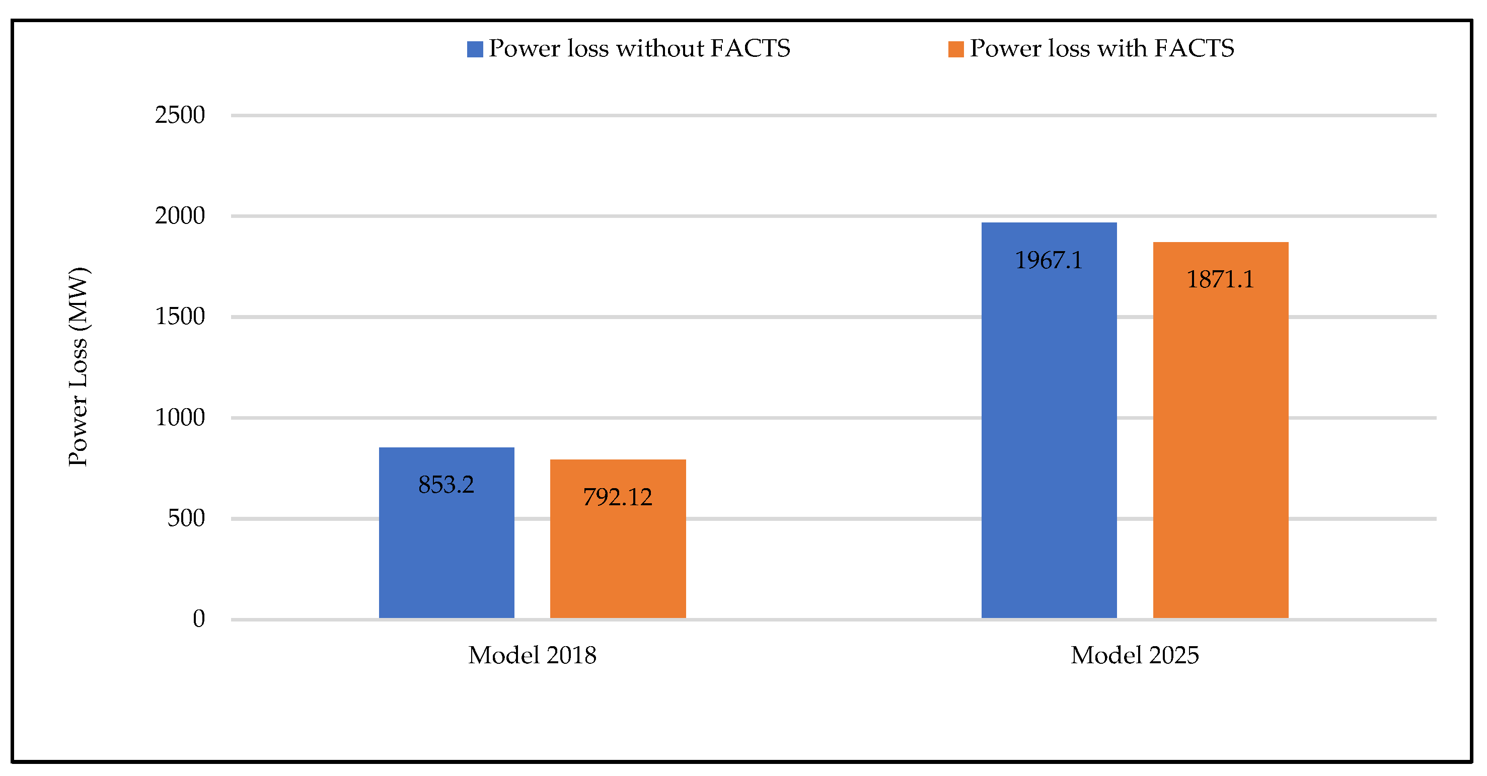
3	System Losses (MW)	853.67	1967.18
4	Mod of SVC Rating	3.1463	3.56
5	Mod of TCSC Rating	0.0705	2.248
6	Total Cost of TCSCs ($)	7.1371 × 103	2.6847 × 107
7	Total Cost of SVCs ($)	6.1815 × 106	7.3795 × 106
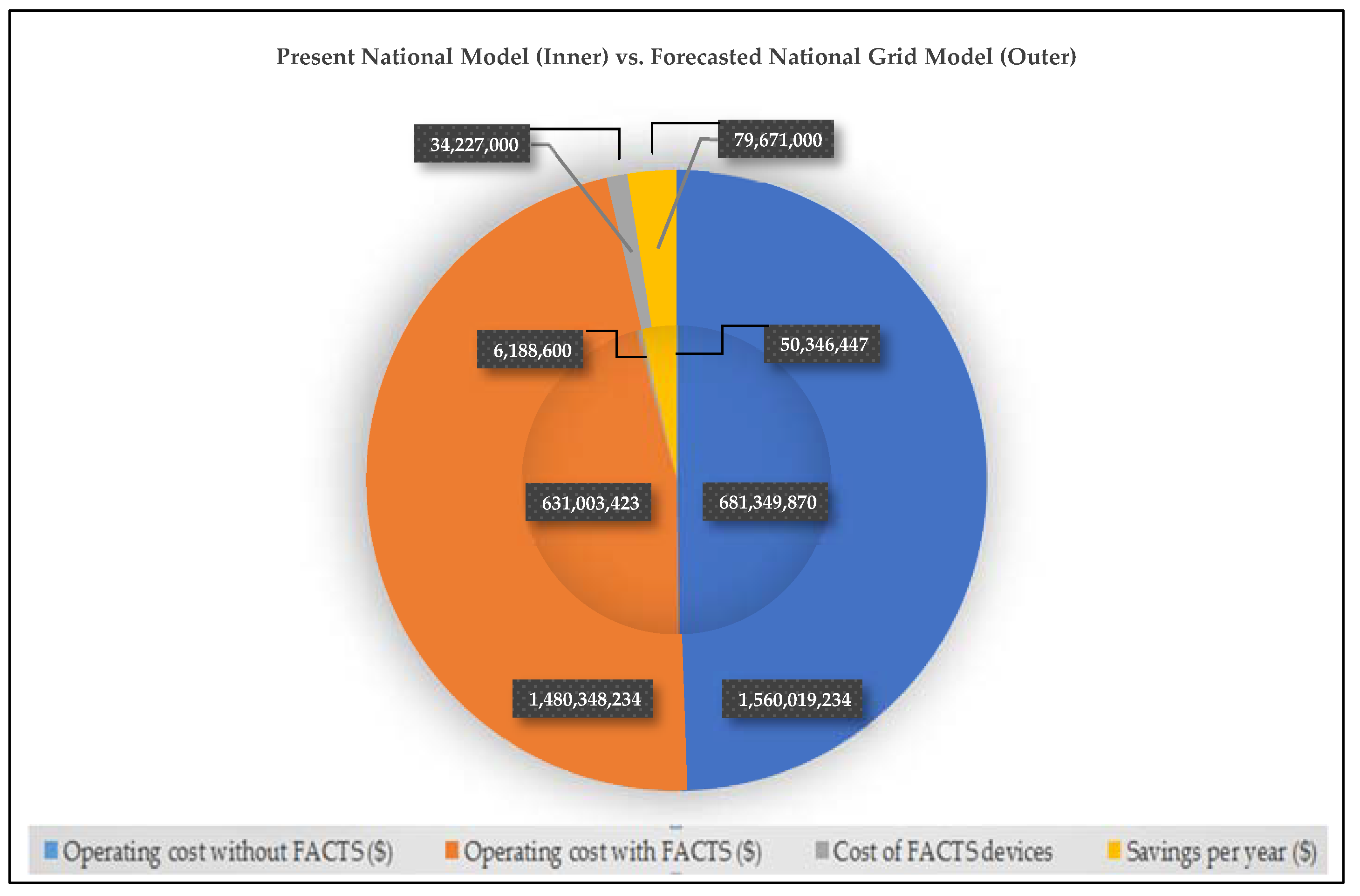
8	Total cost of FACTS devices ($)	6.1886 × 106	3.4227 × 107
9	Payback Period	Less than 1 Year	Less than 1 Year

.

4. Conclusions

In this study, a comprehensive planning model is presented for improving the performance of the national grid for both the present as well as the forecasted scenario by the placement of FACTS devices. Initially, analysis is carried out to find optimum locations of FACTS devices using line stability and voltage collapse proximity indices. Lines with the value of L_mn index close to unity are considered weak lines and candidate locations for TCSC placement. Similarly, buses with VCPI value close to unity are chosen as candidate locations for SVC placement. After finding the candidate locations for FACTS devices, optimal sizes of these devices have been determined using PSO. Results show that an optimized solution significantly reduces power system losses. Active power losses in the Pakistani national grid model 2018 are reduced by 6.21% and the reactive losses by 6.71% using eight TCSCs and six SVCs. The losses can be further reduced by installing more FATCS devices based on the available budget. The voltage profiles for both the present and forecasted grid are improved to a great extent. For the present model, the standard deviation of bus voltages before placement of FACTS is 0.08, which is improved to 0.064 after FACTS placement. Detailed financial analysis, covering the operational cost before and after placement of FACTS as well as the payback period has been calculated. The analysis presented in the current study will serve as the guidelines for policymakers in developing countries to enhance the performance of the national grid for the present and forecasted scenarios.

In future work, it is planned to also include the small-signal stability of the power system in the objective function. Thus, FACTS will be placed and sized to satisfy small-signal stability as well as the objectives achieved in this work.

References

- Almeshqab, F.; Ustun, T.S. Lessons learned from rural electrification initiatives in developing countries: Insights for technical, social, financial and public policy aspects. Renew. Sustain. Energy Rev. 2019, 102, 35–53. [Google Scholar] [CrossRef]
- IRENA. Renewable Capacity Statistics 2019; International Renewable Energy Agency (IRENA): Abu Dhabi, United Arab Emirates, 2019. [Google Scholar]
- Meyabadi, A.F.; Deihimi, M.H. A review of Demand Side Management: Reconsidering theoretical framework. Renew. Sustain. Energy Rev. 2017, 80, 367–379. [Google Scholar] [CrossRef]
- Jabir, H.J.; Teh, J.; Ishak, D.; Abunima, H. Impacts of Demand Side management on Electrical Power Systems: A review. Energies 2018, 11, 1050. [Google Scholar] [CrossRef]
- Bhatti, S.S.; Umair, E.M.; Lodhi, U.; Haq, S. Electric Power Transmission and Distribution Losses Overview and Minimization in Pakistan. Int. J. Sci. Eng. Res. 2015, 6, 1108–1112. [Google Scholar]
- Wood Allen, J.; Bruce, F.; Wollenberg, G.B.S. Power Generation, Operation and Control, 3rd ed.; Wiley-IEEE Press: Piscataway, NJ, USA, 2014; ISBN 9781626239777. [Google Scholar]
- Tauhidi, A.; Chohan, U.W. The Conundrum of Circular Debt; Centre for Aerospace and Security Studies (CASS): Islamabad, Pakistan, 2020. [Google Scholar] [CrossRef]
- Ali, M.; Ahmed, A.B. Multiple-Criteria Policy Anaysis of Circular Debt in Pakistan. In Proceedings of the 2020 International Conference on Engineering and Emerging Technologies (ICEET), Lahore, Pakistan, 22–23 February 2020; pp. 1–7. [Google Scholar]
- Valasai, G.D.; Uqaili, M.A.; Memon, H.U.R.; Samoo, S.R.; Mirjat, N.H.; Harijan, K. Overcoming electricity crisis in Pakistan: A review of sustainable electricity options. Renew. Sustain. Energy Rev. 2017, 72, 734–745. [Google Scholar] [CrossRef]
- National Electric Power Regulatory Authority. State of Industry Report 2020; National Electric Power Regulatory Authority: Islamabad, Pakistan, 2020; Volume 1. [Google Scholar]
- Rafique, M.M.; Rehman, S. National energy scenario of Pakistan—Current status, future alternatives, and institutional infrastructure: An overview. Renew. Sustain. Energy Rev. 2017, 69, 156–167. [Google Scholar] [CrossRef]
- Nawaz, S.; Nasir, I.; Anwar, S. Electricity Demand in Pakistan: A Nonlinear Estimation. Pak. Dev. Rev. 2013, 52, 479–491. [Google Scholar] [CrossRef]
- Shahid, M.; Ullah, K.; Imran, K.; Mahmood, I.; Mahmood, A. Electricity supply pathways based on renewable resources: A sustainable energy future for Pakistan. J. Clean. Prod. 2020, 263, 121511. [Google Scholar] [CrossRef]
- Mubeen, S.E.; Khan, B.; Nema, R.K. Application of Unified Power Flow Controller to Improve Steady State Voltage Limit. IAES Int. J. Robot. Autom. 2017, 6, 277. [Google Scholar] [CrossRef]
- Kavitha, K.; Neela, R. Optimal allocation of multi-type FACTS devices and its effect in enhancing system security using BBO, WIPSO & PSO. J. Electr. Syst. Inf. Technol. 2018, 5, 777–793. [Google Scholar]
- Raj, S.; Bhattacharyya, B. Optimal placement of TCSC and SVC for reactive power planning using Whale optimization algorithm. Swarm Evol. Comput. 2018, 40, 131–143. [Google Scholar] [CrossRef]
- Gaur, D.; Mathew, L. Optimal placement of FACTS devices using optimization techniques: A review. In Proceedings of the 3rd International Conference on Communication Systems (ICCS-2017), Rajasthan, India, 14–16 October 2017; Volume 331. [Google Scholar]
- Kolcun, M.; Čonka, Z.; Beňa, L.; Kanálik, M.; Medveď, D. Improvement of Transmission Capacity by FACTS devices in Central East Europe power system. IFAC-PapersOnline 2016, 49, 376–381. [Google Scholar] [CrossRef]
- Gandoman, F.H.; Ahmadi, A.; Sharaf, A.M.; Siano, P.; Pou, J.; Hredzak, B.; Agelidis, V.G. Review of FACTS technologies and applications for power quality in smart grids with renewable energy systems. Renew. Sustain. Energy Rev. 2018, 82, 502–514. [Google Scholar] [CrossRef]
- Bhole, S.S.; Nigam, P. Improvement of Voltage Stability in Power System by Using SVC and STATCOM. Int. J. Adv. Res. Electr. Electron. Instrum. Eng. 2015, 4, 749–755. [Google Scholar]
- AL Ahmad, A.; Sirjani, R. Optimal placement and sizing of multi-type FACTS devices in power systems using metaheuristic optimisation techniques: An updated review. Ain Shams Eng. J. 2019. [Google Scholar] [CrossRef]
- Bhattacharyya, B.; Kumar, S. Loadability enhancement with FACTS devices using gravitational search algorithm. Int. J. Electr. Power Energy Syst. 2016, 78, 470–479. [Google Scholar] [CrossRef]
- Jmii, H.; Meddeb, A.; Chebbi, S. A combination between FACTS devices for a safe and an economic power system operation. In Proceedings of the 4th International Conference on Control Engineering & Information Technology (CEIT), Hammamet, Tunisia, 16–18 December 2017; pp. 1–6. [Google Scholar] [CrossRef]
- Hermanu, C.; Listiyanto, O.; Ramelan, A. Comparison of Static Var Compensator (SVC) and Unified Power Flow Controller (UPFC) for Static Voltage Stability Based on Sensitivity Analysis: A Case Study of 500 KV Java-Bali Electrical Power System. In Proceedings of the 2019 International Conference on Technologies and Policies in Electric Power & Energy, Yogyakarta, Indonesia, 21–22 October 2019; pp. 1–6. [Google Scholar] [CrossRef]
- Chikkadesai, M.; Allu, D.; Kamalapur, G.D. Comparative Analysis of TCSC and STATCOM in Power System. In Proceedings of the 2018 International Conference on Electrical, Electronics, Communication, Computer and Optimization Techniques (ICEECCOT), Msyuru, India, 14–15 December 2018; pp. 185–190. [Google Scholar] [CrossRef]
- Relic, F.; Maric, P.; Glavas, H.; Petrovic, I. Influence of FACTS device implementation on performance of distribution network with integrated renewable energy sources. Energies 2020, 13, 5516. [Google Scholar] [CrossRef]
- Ramanathan, B.; Elizondo, D.; Enslin, J.; Zhang, L. Cost effective FACTS solution for transmission enhancement and its economic assessment. In Proceedings of the 2006 IEEE/PES Transmission & Distribution Conference and Exposition, Caracas, Venezuela, 15–18 August 2006; pp. 1–6. [Google Scholar] [CrossRef]
- Ghahremani, E.; Kamwa, I. Optimal placement of multiple-type FACTS devices to maximize power system loadability using a generic graphical user interface. IEEE Trans. Power Syst. 2013, 28, 764–778. [Google Scholar] [CrossRef]
- Bansal, H.O.; Agrawal, H.P.; Tiwana, S.; Singal, A.R.; Shrivastava, L. Optimal Location of FACT Devices to Control Reactive Power. Int. J. Eng. Sci. Technol. 2010, 2, 1556–1560. [Google Scholar]
- Panigrahi, B.K.; Suganthan, P.N.; Das, S. Optimal Placement and Sizing of Multi-type Facts Devices Using PSO and HSA. In Proceedings of the International Conference on Swarm, Evolutionary, and Memetic Computing, Bhubaneswar, India, 18–20 December 2014. [Google Scholar]
- Sharma, A.; Chanana, S.; Parida, S. Combined optimal location of FACTS controllers and loadability enhancement in competitive electricity markets using MILP. In Proceedings of the IEEE Power Engineering Society General Meeting, San Francisco, CA, USA, 12–16 June 2005. [Google Scholar]
- Saravanan, M.; Slochanal, S.M.R.; Venkatesh, P.; Prince, S.A.J. Application of PSO technique for optimal location of FACTS devices considering system loadability and cost of installation. In Proceedings of the 2005 International Power Engineering Conference IPEC2005, Singapore, 29 November–2 December 2005. [Google Scholar]
- Jirjees, M.A.; Al-Nimma, D.A.; Al-Hafidh, M.S.M. Voltage Stability Enhancement based on Voltage Stability Indices Using FACTS Controllers. In Proceedings of the International Iraqi Conference on Engineering Technology and Its Applications, IICETA, Al-Najaf, Iraq, 8–9 May 2018. [Google Scholar]
- Nadeem, M.; Imran, K.; Khattak, A.; Ulasyar, A.; Pal, A. Optimal Placement, Sizing and Coordination of FACTS Devices in Transmission Network Using Whale Optimization Algorithm. Energies 2020, 13, 753. [Google Scholar] [CrossRef]
- Araga, I.A.; Anibasa, A.O.; Alabi, I.I. Open Access Placement of Multiple Svc on Nigerian Grid System for Steady State Operational Enhancement. Am. J. Eng. Res. 2017, 6, 78–85. [Google Scholar]
- Alsheikh, M.; Osman, A. Contingency Analysis in Presence of SVC Controller of Sudan National Grid for Electricity. Ph.D. Thesis, University of Science and Technology, Omdurman, Sudan, 2018. [Google Scholar]
- Al-rubayi, R.H.; Ibrahim, L.G. Optimal Placement of FACTs Devices in Iraqi National Super Grid System (INSGS) Using HLSI. Int. J. Eng. Technol. Sci. 2019, 6, 100–114. [Google Scholar]
- Zimmerman, R.D.; Murillo-Sánchez, C.E.; Thomas, R.J. MATPOWER: Steady-state operations, planning, and analysis tools for power systems research and education. IEEE Trans. Power Syst. 2011, 26, 12–19. [Google Scholar] [CrossRef]
- Nuchhi, S. Comparative Study of TCSC and SVC for Power System. Int. J. Recent Adv. Eng. Res. 2017, 3, 1. [Google Scholar] [CrossRef]
- Nadeem, M.; Zeb, M.Z.; Imran, K.; Janjua, A.K. Optimal Sizing and Allocation of SVC and TCSC in Transmission Network by combined Sensitivity index and PSO. In Proceedings of the 2019 International Conference on Applied and Engineering Mathematics (ICAEM), London, UK, 3–5 July 2019; pp. 111–116. [Google Scholar]
- Anwar, Z.; Malik, T.N.; Sarfraz, A.; Hameed, H.; Rehman, A.; Abbas, T. Applications of FACTS/ESS in Power System Congestion Management with Large Renewable Energy Sources Using PSS/E and Experienced in National Grid of Pakistan. J. Appl. Emerg. Sci. 2018, 8, 77–95. [Google Scholar]
- Padiyar, K.R. Facts Controllers in Power Transmission Distribution; New Age Internatopnal (P) Limited: New Delhi, India, 2007; ISBN 9788122425413. [Google Scholar]
- National Electric Power Regulatory Authority Consumer-End Applicable Tariff. Available online: https://nepra.org.pk/consumeraffairs/ElectricityBill.php (accessed on 15 January 2021).
- James Kennedy, R.E. Particle Swarm Optimization. In Proceedings of the ICNN’95-International Conference on Neural Networks, Perth, WA, Australia, 27 November–1 December 1995. [Google Scholar]
- Bhattacharyya, B.; Kumar, S. Approach for the solution of transmission congestion with multi-type FACTS devices. IET Gener. Transm. Distrib. 2016, 10, 2802–2809. [Google Scholar] [CrossRef]
- National Electric Power Regulatory Authority. State of Industry Report; National Electric Power Regulatory Authority: Islamabad, Pakistan, 2018. [Google Scholar]