Energetic Performances Booster for Electric Vehicle Applications Using Transient Power Control and Supercapacitors-Batteries/Fuel Cell

Abstract

In this paper, a hybrid electric power supply system for an electric vehicle (EV) is investigated. The study aims to reduce electric stress on the main energy source (fuel cell) and boost energetic performances using energy sources with high specific power (supercapacitors, batteries) for rapid traction chain solicitations such as accelerations, decelerations, and braking operations. The multisource EV power supply system contains a fuel cell stack, a lithium batteries module, and a supercapacitors (Sc) pack. In order to emulate the EV energy demand (wheels, weight, external forces, etc.), a bidirectional load based on a reversible current DC-DC converter was used. Fuel cell (Fc) stack was interfaced by an interleaved boost converter. Batteries and the Sc pack were coupled to the DC point of coupling via buck/boost converters. Paper contribution was firstly concentrated on the distribution of energy and power between onboard energy sources in consonance with their dynamic characteristics (time response). Second contribution was based on a new Sc model, which takes into consideration the temperature and the DC current ripples frequency until 1000 Hz. Energy management strategy (EMS) was evaluated by simulations and reduced scale experimental tests. The used driving cycle was the US Federal Test Procedure known as FTP-75.

1. Introduction

The insufficient performance of actual electric vehicle (EV) energy storage technologies is one of the main restrictions to their advancement [1]. Despite the fact that greenhouse gas emissions are locally zero for EVs, their success will only be possible if they at least offer the same performances as those provided by internal combustion engine (ICE) vehicles, namely: a good autonomy, a short charging time, a large torque over a wide speed range, and a reasonable cost. These performances will only be possible if the onboard energy storage system has a high power density, a high energy density, an affordable cost, and a reasonable weight and volume. Currently, no electric energy storage device is able to ensure all these performances by itself [2]. Among all the available electrical energy storage technologies, in lithium batteries, the fuel cell (Fc) and supercapacitors (Sc) are mainly intended for transport applications and more specifically for EVs and Hybrid Electric Vehicles (HEV). The batteries have generally a good energy density (specific energy), which ensures a relatively good autonomy for the EV. However, their low power density (specific power) makes them vulnerable to the vehicle peak power solicitations. The batteries’ dynamic response remains insufficient compared to the EV traction chain demands, consequently, the batteries’ life span will be greatly compromised. In addition, they are relatively expensive, they require a long charging time, and they are responsible for a significant part of the vehicle weight. Currently, lithium battery technologies are the EV manufacturer’s first choice. Compared to other technologies, LiFePO₄ batteries offer an interesting arrangement between electrical performances, environmental impact, and investment cost. Being accompanied by a hydrogen tank, fuel cells are known for their high specific energy and good energy autonomy similar to ICE vehicles is then possible. Fuel cell specific energy is greater than the battery one. However, Fc has a poor specific power, which makes them unable to match the EV typical accelerations power needs. In addition, the energy produced during the decelerations and braking operations cannot be recovered by the Fc due to unidirectional behavior. The Fc system remains too expensive and complex due to the auxiliary components necessary for its functioning. Furthermore, the construction of a large hydrogen distribution network similar to that of gas stations is indeed a huge investment. The supercapacitors (Sc) have different characteristics from those of the batteries and fuel cells. Thanks to their higher specific power, they are considered a “power source”, but their specific energy is inadequate to afford the EV energy autonomy. Electric energy storage technology within the Sc is predominantly based on electrostatic phenomena. This characteristic gives them a good dynamic response to load requests with a considerable number of charge–discharge cycles [3,4]. Based on the energy sources’ intrinsic characteristics described above, complementary energetic performances between the Sc, Fc, and batteries are distinguished [5]. So far, there’s no energy source that combines all the desired performances for EV applications and which can permit the drivers to obtain a good energy autonomy akin to conventional vehicles. For these reasons, energy source hybridization is an effective solution. On one hand, EV applications require a good energy density, which is an important feature to satisfy the EV autonomy, and this characteristic can be provided by the batteries or the fuel cells. On the other hand, to match the high accelerations power requirements and to store the energy produced during the decelerations and regenerative braking operations, a high power density storage unit such as Sc or high specific power batteries will be of great use [6]. In order to respect the energy source characteristics, an adequate energy management strategy (EMS) is necessary to control the contribution of the onboard energy sources through the interfaced power converters to ensure their optimal operations and durability [7,8]. This paper deals with the electrical energy storage systems hybridization with a focus on the EMS within the onboard energy storage system (ESS) in order to satisfy the EV requirements and protect the Fc state-of-health (SoH). In the literature, different configurations and different EMS are proposed for multi-source systems [9,10,11,12,13,14,15,16,17], such as battery-Sc configuration with real-time bi-adaptive controller [15], fuel cell-Sc-based hybrid electric vehicles with adaptive EMS [16], Fc-battery energy system with operating states EMS [17]. In comparison with the cited hybrid systems architectures, the adopted EV configuration is based on a battery-Sc-Fc architecture [10,11,12,13,14], as illustrated in Figure 1.This configuration contains an Fc module associated to DC-link through the medium of a three-channel interleaved boost converter. The Fc ensures the EV energetic autonomy as well as the DC-link voltage control. The battery module and the Sc pack are the vehicle’s auxiliary energy sources. They are interfaced to the DC-link using buck/boost converters. They assist Fc during accelerations where the EV requires large amounts of energy within a short duration. In addition, the batteries and Sc allow recovering the energy produced during decelerations and braking phases. The EV power demands due to (weight, external forces...) are emulated using a bidirectional controlled DC load.

This paper’s contribution, as compared to the literature, is focused on the coordinated transient power control for electric vehicle power demand distribution according to the onboard energy sources’ time response and their state of health. Thus, the energy sources operate with adapted time-responses to their intrinsic characteristics and the fast aging phenomena is limited. Another important contribution concerns the new Sc behavioral model, which includes the influence of temperature and DC-current ripples frequency until 1000 Hz. The new model allows to better understand supercapacitors behavior towards using conditions variations such as temperature and current wave form, which are the main electric performance degrading factors.

This paper is organized as following: after the introduction, the energy sources behavioral models are described in Section 2. Energy management method and the power converters control are detailed in Section 3. Simulations and reduced-scale experimental tests results are presented in Section 4. Paper conclusion is presented in Section 5.

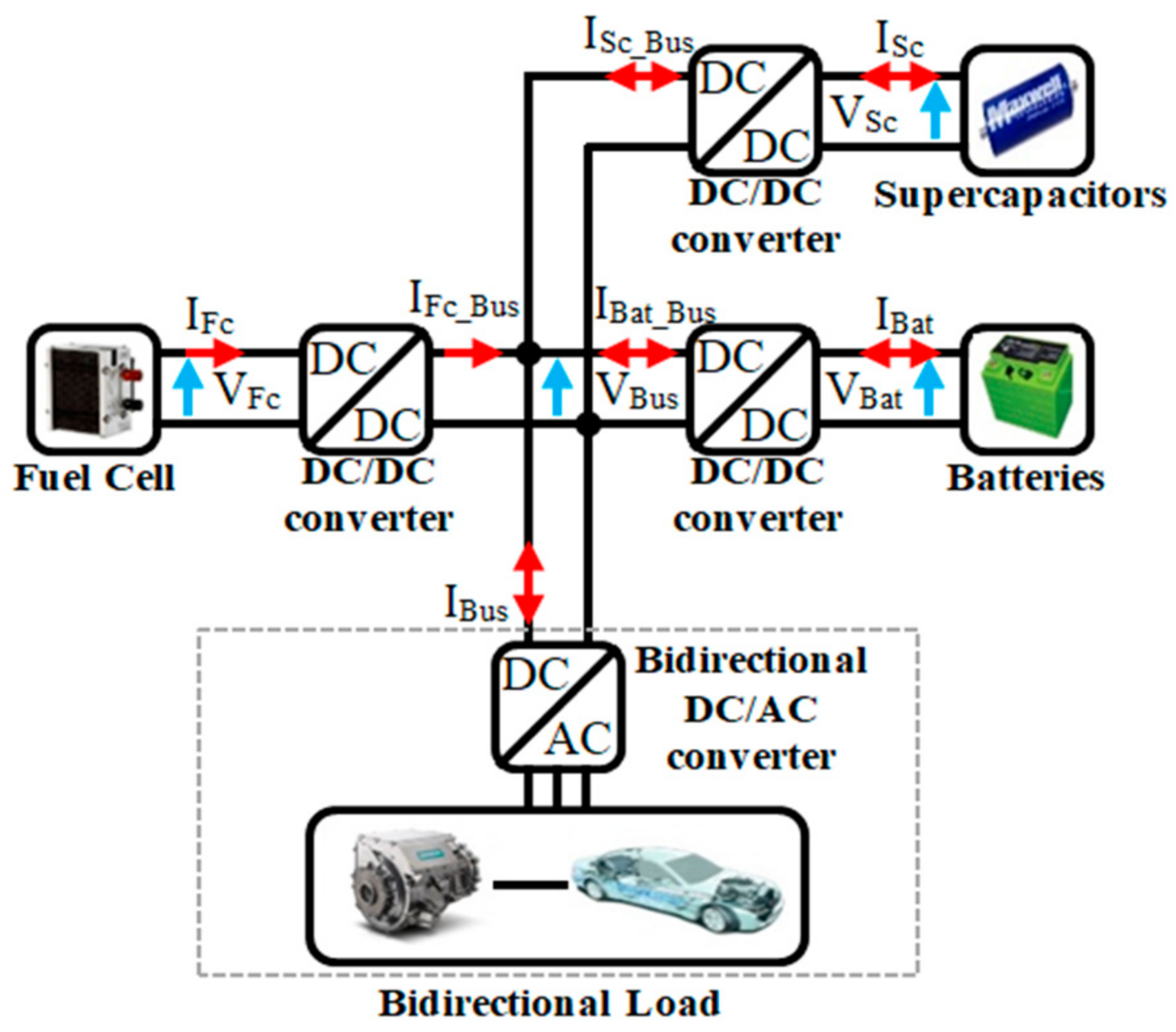
2. Model of the Sources

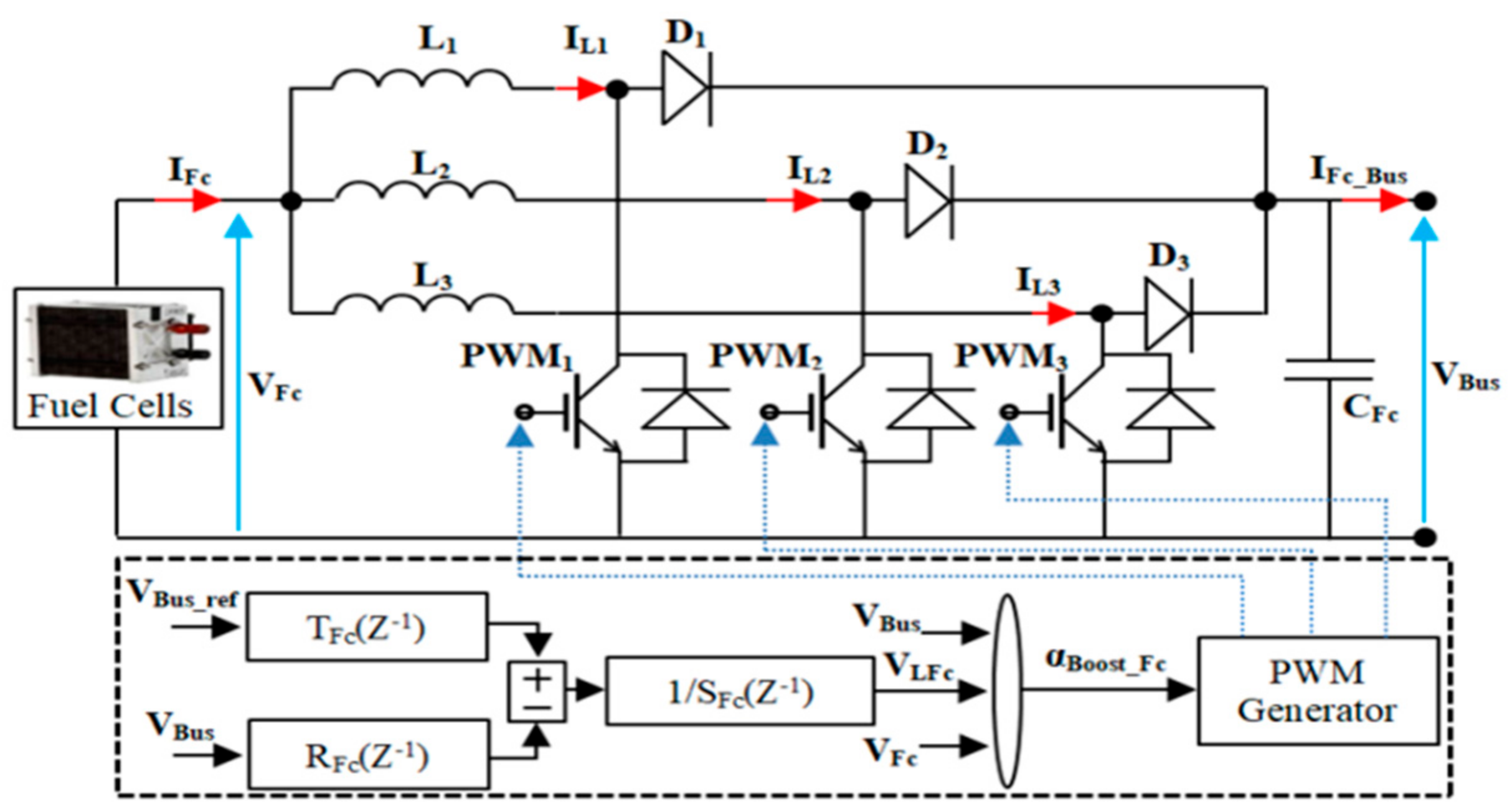
2.1. Model of Proton-Exchange Membrane Fuel Cells

Among the various fuel cell technologies, Proton-Exchange Membrane Fuel Cells (PEMFCs) are the most used for transport applications. They have been used in different applications such as: scooters, planes, buses, and more particularly for EVs and HEVs [18,19]. Fuel cells are known for their high specific energy. However, their specific power is low compared to energy storage technologies. The life expectancy of fuel cells can be quickly compromised if they are subject to significant solicitations with large DC-current ripples. The used model of the Fc extracted from [20] is presented in Equation (1), where E₀ presents thermodynamic potential for a cell, V_Act presents the voltage drop caused by activation of the anode and the cathode, V_Ohm presents the voltage drop in series resistance, V_Con corresponds to voltage drop caused by the concentrations, N_{S_Fc} presents the cell number in series.

$$\{\begin{array}{l}{V}_{Fc}=N_{S\_Fc}\ast \left(E_0-V_{Act}-V_{Ohm}-V_{Conc}\right)\\ E_0=1.229-\frac{0.85}{{10}^3}\ast (T-298.15)+\frac{4.308}{{10}^5}\ast T\ast [\ln ({\mathrm{P}}_{H2})+0.5\ast \ln ({\mathrm{P}}_{O2})]\hspace{0.17em}\\ V_{Act}=-[{\lambda }_1+{\lambda }_2\ast T+{\lambda }_3\ast T\ast \ln (C_{O2})+{\lambda }_4\ast T\ast \ln (I_{Fc})]\\ C_{O2}=\frac{{\mathrm{P}}_{O2}}{5.08\ast {10}^6\ast {\mathrm{e}}^{\frac{-498}{T}}}\\ V_{Ohm}=I_{Fc}\ast \left(R_{el}-R_p\right)\\ V_{Con}=-{\beta }_1\ast \ln \left(1-\raisebox{1ex}{$J$}\!\left/ \!\raisebox{-1ex}{$J_{\max }$}\right.\right)\\ R_p=\frac{r_m}{A_r}\ast L\\ r_m=\frac{181.6\ast \left[1+\frac{3}{{10}^2}\ast \left(\raisebox{1ex}{$i$}\!\left/ \!\raisebox{-1ex}{$A_r$}\right.\right)+\frac{62}{{10}^2}\ast {\left(\frac{T}{303}\right)}^2\ast {\left(\raisebox{1ex}{$i$}\!\left/ \!\raisebox{-1ex}{$A_r$}\right.\right)}^{2.5}\right]}{\left[\gamma -0.63-3\ast \left(\raisebox{1ex}{$i$}\!\left/ \!\raisebox{-1ex}{$A_r$}\right.\right)\ast {\mathrm{e}}^{4.18\ast \left(1-\frac{303}{T}\right)}\right]}\end{array}$$

(1)

In Equation (1), T presents the temperature in [K], P_H2 and P_O2 are the pressures of hydrogen and oxygen in [atm], I_Fc is the fuel cell current, λ₁ to λ₄ are parametric coefficients, C_O2 presents oxygen concentration, J presents current density in [A/cm²], β₁ is a constant parameter, R_el is the resistance due to electrons flow, R_p is the resistance due to protons flow, L is the polymer membrane thickness in [cm], A_r presents the active cell area in [cm²], r_m presents the specific resistivity due to hydrated protons in [Ω.cm] and γ presents membrane humidity ratio, and V_Fc is the Fc terminal voltage. All Fc model parameters are given in

Table 1. Fuel cell parameters.

Description	Symbol	Parameters
Parametric coefficients	λ1; λ2 λ3; λ4	−0.984; 0.00312 7.22 × 10−5; −1.061 × 10−4
Electron flow resistance	Rel	3 × 10−4 Ω
Pressures of O2 and H2	PO2; PH2	0.209 atm; 1.476 atm
Polymer membrane thickness	L	25 × 10−4 cm
Fc active area	Ar	67 cm2
Maximum current density	Jmax	0.672 A/cm2
Constant parameter	β1	0.15
Cells number in series	NS_Fc	288

.

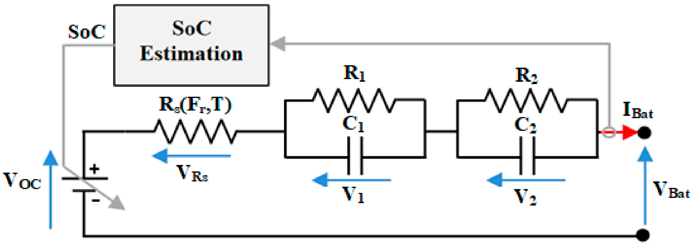
2.2. Model of LiFePO₄ Batteries

In this paper, a model dedicated to lithium iron phosphate batteries was used. This type of batteries presents an interesting solution in terms of investment cost associated to required energetic performances [21]. The used model of the batteries is shown in Figure 2. It contained an open circuit voltage Voc, which depends on the state of charge SoC and the sign of the battery’s current, a series resistance R_S(F_r,T), and two parallel RC circuits. The model contained two time constants, which remained invariable during the battery operations. The resistances and capacitances of the parallel RC circuits (R₁//C₁ and R₂//C₂) were assumed constant. The first time constant related the batteries behavior for short time durations. The second time constant was used to describe the batteries behavior for long-time horizons.

$$\{\begin{array}{l}\\ SoC=\{\begin{array}{l}SoC(t_0)+{\displaystyle {\int }_{t_0}^t\left(\frac{I_{Bat}}{3600\ast Q_{cell\_ch}(F_r,T)}\right)·dt}\begin{array}{cc}& \end{array}for\begin{array}{cc}& I_{Bat}<0\end{array}\\ SoC(t_0)-{\displaystyle {\int }_{t_0}^t\left(\frac{I_{Bat}}{3600\ast Q_{cell\_di}(F_r,T)}\right)·dt}\begin{array}{cc}& \end{array}for\begin{array}{cc}& I_{Bat}>0\end{array}\end{array}\\ \frac{d}{dt}\left[\begin{array}{l}{V}_1\\ V_2\end{array}\right]=\left[\begin{array}{cc}-\frac{1}{R_1\ast C_1}& 0\\ 0& -\frac{1}{R_2\ast C_2}\end{array}\right]\ast \left[\begin{array}{l}{V}_1\\ V_2\end{array}\right]+\left[\begin{array}{cc}\frac{1}{C_1}& 0\\ \frac{1}{C_2}& 0\end{array}\right]\ast \left[\begin{array}{l}{I}_{Bat}\\ 0\end{array}\right]\\ R_s(F_r,T)=\frac{N_{S\_Bat}}{N_{p\_Bat}}\ast R_{Cell}\left(F_r,T\right)+\frac{\left(N_{S\_Bat}-1\right)}{N_{p\_Bat}}\ast R_{bwi}\\ V_{oc}(SoC)=\{\begin{array}{l}-c_5\ast So{C}_{}^5+c_4\ast So{C}_{}^4-c_3\ast So{C}_{}^3+c_2\ast So{C}_{}^2+c_1\ast So{C}_{}^{}+c_0{{\displaystyle }}_{}for{{\displaystyle {}_{}}}_{}{I}_{Bat}<0\\ -d_5\ast So{C}_{}^5+d_4\ast So{C}_{}^4-d_3\ast So{C}_{}^3+d_2\ast So{C}_{}^2-d_1\ast So{C}_{}^{}+d_0{{\displaystyle }}_{}for{{\displaystyle }}_{}{I}_{Bat}>0\end{array}\\ V_{Bat}=N_{S\_Bat}\ast V_{oc}\left(SoC\right)+\left(\frac{N_{S\_Bat}}{N_{p\_Bat}}\right)\ast \left(R_s\ast I_{Bat}+V_1+V_2\right)\end{array}$$

(2)

The LiFePO₄ battery model is based on one battery cell with the rated parameters of LFP-100 Ah/3.2 V. The detailed characterization method is described in [22]. The analytical model of the batteries is presented in Equation (2), where N_{S_Bat} and N_{P_Bat} are the number of batteries in series and parallel. The coefficients of the V_OC(SoC) corresponding to the charge (I_Bat < 0) and discharge (I_Bat > 0) operations are: c₀ = 0.9; c₁ = 4.8; c₂ = 33; c₃ = 140; c₄ = 179; c₅ = 74; d₀ = 1; d₁ = 0.7; d₂ = 42; d₃ = 132; d₄ = 15; d₅ = 62. The parameters of the batteries model are given in

Table 2. Parameters of LiFePO₄-batteries model.

Description	Symbol	Parameters
Operating voltage range for battery cell	VBatmin~VBatmax	2.8 V~3.8 V
Resistance of the first parallel RC	R1	0.033 Ω
Capacitance of the first parallel RC	C1	92 F
Resistance of the second parallel RC	R2	0.375 Ω
Capacitance of the second parallel RC	C2	499 F
Specific power	$\rho$PBat	310 W/Kg
Specific energy	$\rho$EBat	102 Wh/Kg
Battery State of Charge (SoC) initial value	SoC(t0)	97%
Number of elements in series	Ns_Bat	59
Number of elements in parallel	NP_Bat	1
Resistance due to electric wiring for one battery	Rbwi	4.5 m Ω

.

LFP-100 Ah battery resistance and capacitance were achieved from 4800 cycles of charge-discharge tests, as presented in Equation (3), where F_r is the DC current ripples frequency in [Hz].

$$\{\begin{array}{l}{\mathrm{R}}_{\mathrm{cell}}{(\mathrm{F}}_r,\mathrm{T})=\frac{1}{1000}\ast \left(\begin{array}{l}{\mathrm{r}}_0{+\mathrm{r}}_{10}\ast {\mathrm{F}}_r{+\mathrm{r}}_{01}\ast {\mathrm{T}+\mathrm{r}}_{20}\ast {\mathrm{F}}_r{}^2{+\mathrm{r}}_{11}\ast {\mathrm{F}}_r\ast {\mathrm{T}+\mathrm{r}}_{02}\ast {\mathrm{T}}^2+{\mathrm{r}}_{30}\ast {\mathrm{F}}_r{}^3\\ {+\mathrm{r}}_{21}\ast {\mathrm{F}}_r{}^2\ast {\mathrm{T}+\mathrm{r}}_{12}\ast {\mathrm{F}}_r\ast {\mathrm{T}}^2\end{array}\right)\\ {\mathrm{Q}}_{\mathrm{cell}\_\mathrm{ch}}{(\mathrm{F}}_r,\mathrm{T})\approx {\mathrm{Q}}_{\mathrm{cell}\_\mathrm{di}}{(\mathrm{F}}_r{,\mathrm{T})=\mathrm{q}}_0{+\mathrm{q}}_{10}\ast {\mathrm{F}}_r{+\mathrm{q}}_{01}\ast {\mathrm{T}+\mathrm{q}}_{20}\ast {\mathrm{F}}_r{}^2{+\mathrm{q}}_{11}\ast {\mathrm{F}}_r\ast {\mathrm{T}+\mathrm{q}}_{02}\ast {\mathrm{T}}^2\end{array}$$

(3)

The coefficients of Equation (3) with 95% confidence bounds are given as follows: r₀ = 2.263; r₁₀ = 0.4496; r₀₁ = −0.5637; r₂₀ = −0.472; r₁₁ = −0.145; r₀₂ = 0.3145; r₃₀ = 0.1441; r₂₁ = 0.1523; r₁₂ = −4.14 × 10⁻²; q₀ = 84; q₁₀ = 1.01; q₀₁ = 1.50; q₂₀ = −0.158; q₁₁ = −0.222; q₀₂ = −0.0148. The battery model enabled to describe the LFP-batteries behavior when they were submitted to both electrical and thermal constraints.

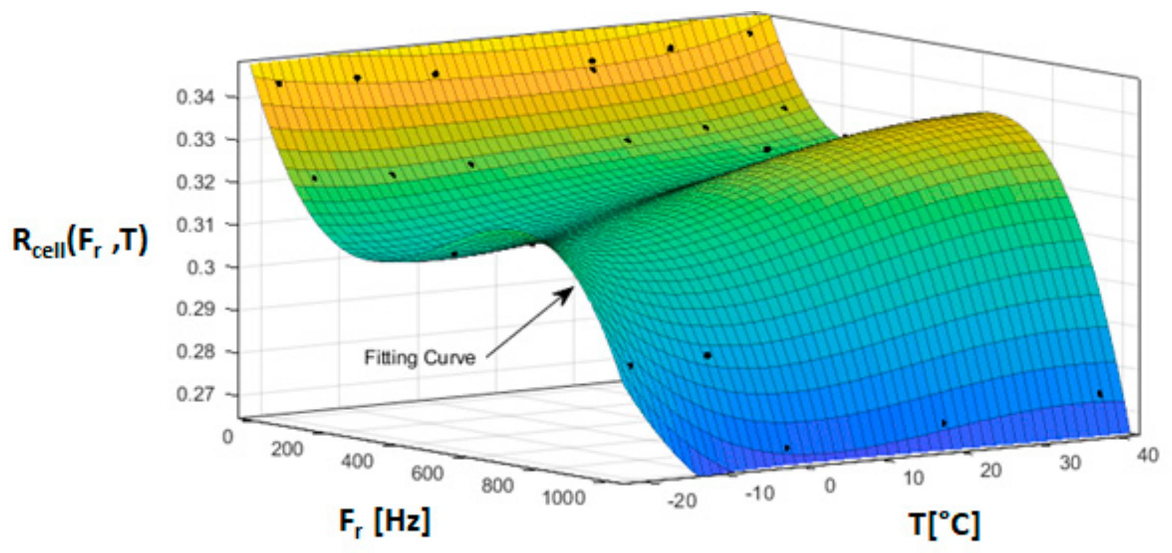
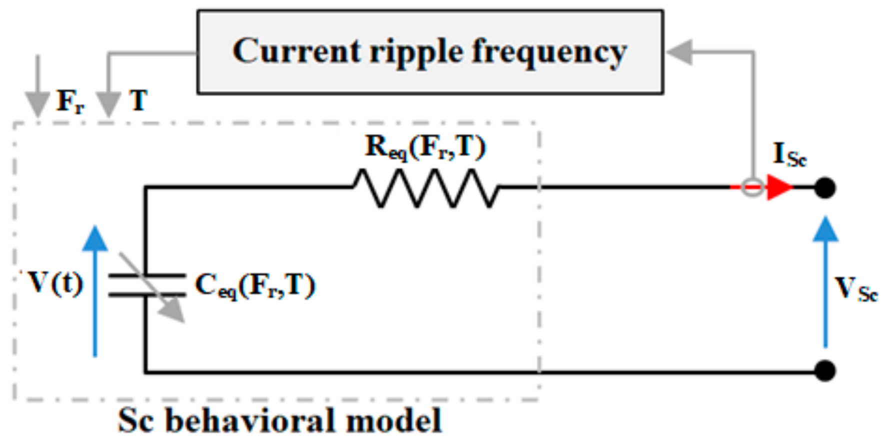
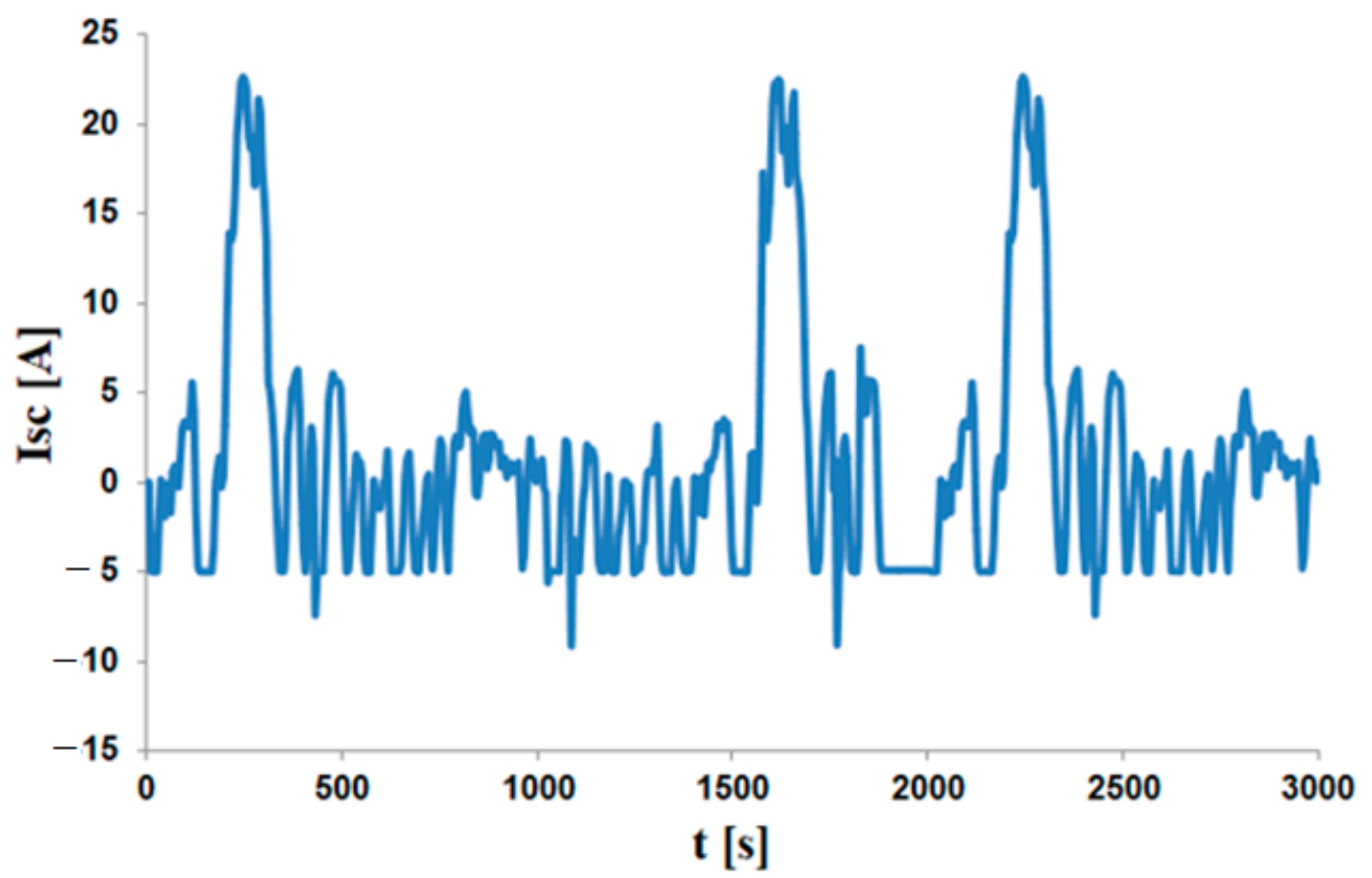
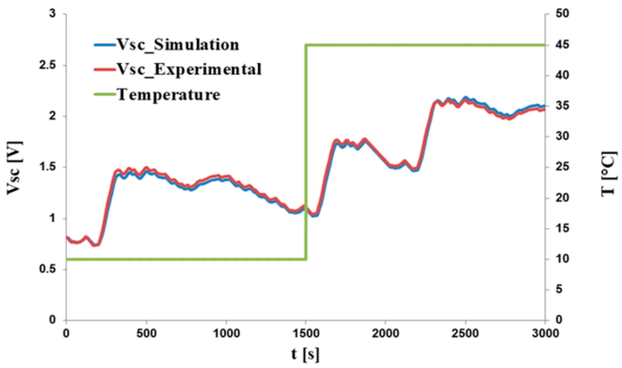
2.3. Supercapacitors Characterization and Modeling

The Sc behavior characterization was based on experimental charge/discharge tests performed with fluctuating DC current waveforms and different levels of temperature. In the literature, several Sc model were proposed [23,24,25,26], although these models were limited in critical conditions of use, in some case the Sc capacitance and resistance were constant or the multisource system real constraints were not considered. The aim of the characterization method was to evaluate the Sc parameters (capacitance and resistance) variations based on the frequency of DC current ripples (F_r) and temperature in order to establish a model that takes into account these constraints. The characterization method was firstly based on electrochemical impedance spectroscopy (EIS) cycling tests using different values of F_r for Sc cell charge/discharge and over 500 cycles. Secondly, in order to determine the Sc impedance, the tests were performed using a fixed DC voltage value superimposed to a low amplitude sinusoidal voltage with a frequency range of 1 mHz to 1 kHz. The resulting voltage was applied to the Sc cell to measure the impedance, which was used to determine the Sc cell capacitance C_cell and its resistance R_cell. To impose the thermal constraints, a climatic chamber was used to regulate the temperature to the following values in [°C]: −20, −10, 0, 20, 30, and 40. For cycling tests, F_r was fixed to: 0.5 Hz, 1 Hz, 0.1 kHz, 0.5 kHz, and 1 kHz. The performed tests made it possible to obtain the Sc cell impedance evolution in order to identify R_eq and C_eq. Sc cell resistance and capacitance were computed using Equation (4), where Im(Z) and Re(Z) present imaginary and real components of the impedance [27].

$$\{\begin{array}{l}{C}_{cell}=\frac{-1}{2\ast \pi \ast f\ast \mathrm{Im}(Z)}\\ R_{cell}=\min (\mathrm{Re}(Z))\end{array}\hspace{0.17em}$$

(4)

The Sc cell parameters were identified allowing the evolution representation of R_cell(F_r,T) in [mΩ] and C_cell(F_r,T) in [F] according to electro-thermal constraints. The Sc cell resistance and capacitance variations based on temperature and F_r are illustrated in Figure 3 and Figure 4.

Matlab curve fitting Toolbox was used to obtain the Sc cell resistance and capacitance as function of temperature and frequency as presented in Equations (5).

$$\{\begin{array}{l}{\mathrm{R}}_{\mathrm{cell}}{(\mathrm{F}}_r,\mathrm{T})=\frac{1}{1000}\ast \left(\begin{array}{l}{\mathrm{b}}_0{-\mathrm{b}}_1\ast {\mathrm{F}}_r{-\mathrm{b}}_2\ast {\mathrm{T}+\mathrm{b}}_3\ast {\mathrm{F}}_r{}^2{+\mathrm{b}}_4\ast {\mathrm{F}}_r\ast {\mathrm{T}+\mathrm{b}}_5\ast {\mathrm{T}}^2-{\mathrm{b}}_6\ast {\mathrm{F}}_r{}^3{-\mathrm{b}}_7\ast {\mathrm{F}}_r{}^2\ast {\mathrm{T}-\mathrm{b}}_8\ast {\mathrm{F}}_r\ast {\mathrm{T}}^2\\ -{\mathrm{b}}_9\ast {\mathrm{T}}^3-{\mathrm{b}}_{10}\ast {\mathrm{F}}_r^3\ast \mathrm{T}+{\mathrm{b}}_{11}\ast {\mathrm{F}}_r^2\ast {\mathrm{T}}^2-{\mathrm{b}}_{12}\ast {\mathrm{F}}_r\ast {\mathrm{T}}^3+{\mathrm{b}}_{13}\ast {\mathrm{T}}^4\end{array}\right)\\ {\mathrm{C}}_{\mathrm{cell}\_\mathrm{ch}/\mathrm{di}}{(\mathrm{F}}_r{,\mathrm{T})=\mathrm{a}}_0{-\mathrm{a}}_1\ast {\mathrm{F}}_r{+\mathrm{a}}_2\ast {\mathrm{T}+\mathrm{a}}_3\ast {\mathrm{F}}_r{}^2{-\mathrm{a}}_4\ast {\mathrm{F}}_r\ast {\mathrm{T}-\mathrm{a}}_5\ast {\mathrm{T}}^2-{\mathrm{a}}_6\ast {\mathrm{F}}_r{}^3+{\mathrm{a}}_7\ast {\mathrm{F}}_r{}^2\ast \mathrm{T}+{\mathrm{a}}_8\ast {\mathrm{F}}_r\ast {\mathrm{T}}^2+{\mathrm{a}}_9\ast {\mathrm{T}}^3\end{array}$$

(5)

Polynomial coefficients of Equations (5) are given as follows: b₀ = 339.9; b₁ = 2.283 × 10⁻¹; b₂ = 6.217 × 10⁻²; b₃ = 5.616 × 10⁻⁴; b₄ = 1.616 × 10⁻³; b₅ = 2.671 × 10⁻³; b₆ = 4.045 × 10⁻⁷; b₇ = 5.285 × 10⁻⁸; b₈ = 1.536 × 10⁻⁵; b₉ = 7.912 × 10⁻⁵; b₁₀ = 1.761 × 10⁻⁹; b₁₁ = 4.289 × 10⁻⁸; b₁₂ = 5.554 × 10⁻⁷; b₁₃ = 3.215 × 10⁻⁶; a0 = 1237; a₁ = 1.633; a₂ = 10.46; a₃ = 3.945 × 10⁻³; a₄ = 0.04636; a₅ = 0.1533; a₆ = 2.225 × 10⁻⁶; a₇ = 4.079 × 10⁻⁵; a₈ = 2.984 × 10⁻⁴; a₉ = 1.233 × 10⁻².

Figure 3 and Figure 4 show a good correlation between experimental data and the curve fitting. The Sc cell resistance R_cell(F_r,T) decreased when the DC current ripples frequency increased. Sc cell capacitance C_cell(F_r,T) increased when F_r and temperature increased. Sc pack behavior model is presented in Figure 5. This model contains an equivalent series resistance R_eq(F_r,T) and an equivalent capacitance C_eq(F_r,T). These parameters depended on the temperature and the F_r. Sc analytical model is given in Equation (6), where N_{S_Sc} and N_{P_Sc} are the number of the Sc cells in series and parallel. R_cell(F_r,T) and C_cell(F_r,T) present the Sc cell resistance and capacitance. R_wi presents wiring resistance between two consecutive cells and V_Sc0 is the Sc cell initial voltage. The proposed model’s main advantage compared to the literature was the consideration of the current waveform frequency and temperature as degradation factors for the Sc parameters (capacitance and resistance). The main Sc model parameters are given in

Table 3. Sc model parameters based on Boostcap 3000F/2.7V cell.

Description	Symbol	Parameters
Operating voltage range for Sc cell	VScmin~VScmax	0.7 V~2.7 V
Specific power	$\rho$PSc	5900 W/kg
Specific energy	$\rho$ESc	6 Wh/kg
Initial value of SoC	SoC(t0)	70%
Number of cells in series	Ns_Sc	70
Number of cells in parallel	NP_Sc	1
Resistance due to electric wiring for one cell	Rwi	4.47 m Ω

.

$$\{\begin{array}{l}{V}_{Sc}=N_{s\_Sc}\ast V_{Sc}{}_0-{\displaystyle \underset{0}{\overset{t}{\int }}\frac{I_{Sc}}{{\mathrm{C}}_{\mathrm{eq}}\left(F_r,T\right)}}\ast dt-{\mathrm{R}}_{\mathrm{eq}}\left(F_r,T\right)\ast I_{Sc}\\ {\mathrm{C}}_{\mathrm{eq}}\left(F_r,T\right)=\frac{N_{p-Sc}}{N_{s-Sc}}\ast C_{cell}(F_r,T)\\ R_{eq}\left(F_r,T\right)=\frac{N_{S\_Sc}}{N_{p\_Sc}}\ast R_{cell}(F_r,T)+\frac{\left(N_{S\_Sc}-1\right)}{N_{p\_Sc}}\ast R_{wi}\end{array}$$

(6)

The Sc cell model verification was done using a DC-current profile based on FTP-75 driving cycle and the Volkswagen e-UP vehicle model, the used current profile is illustrated in Figure 6. To show the temperature impact on resistance and capacitance, Sc temperature was respectively fixed to 10 and 45 °C through the climatic chamber as plotted in Figure 7. The simulations results compared to experimental data for one cell are presented in Figure 7, where the Sc cell terminal voltages obtained from experimental and simulation tests were close to each other, the gap between the two voltage results was lower than 5%. Figure 8 presents the parametric study of the proposed Sc behavior model. The capacitance decreased from 2960 F to 2860 F and the resistance increased from 0.258 to 0.274 mΩ. These results enabled the authors to conclude that the proposed model reproduced well the Sc behavior in charge/discharge operations, taking into consideration the Sc aging factors.

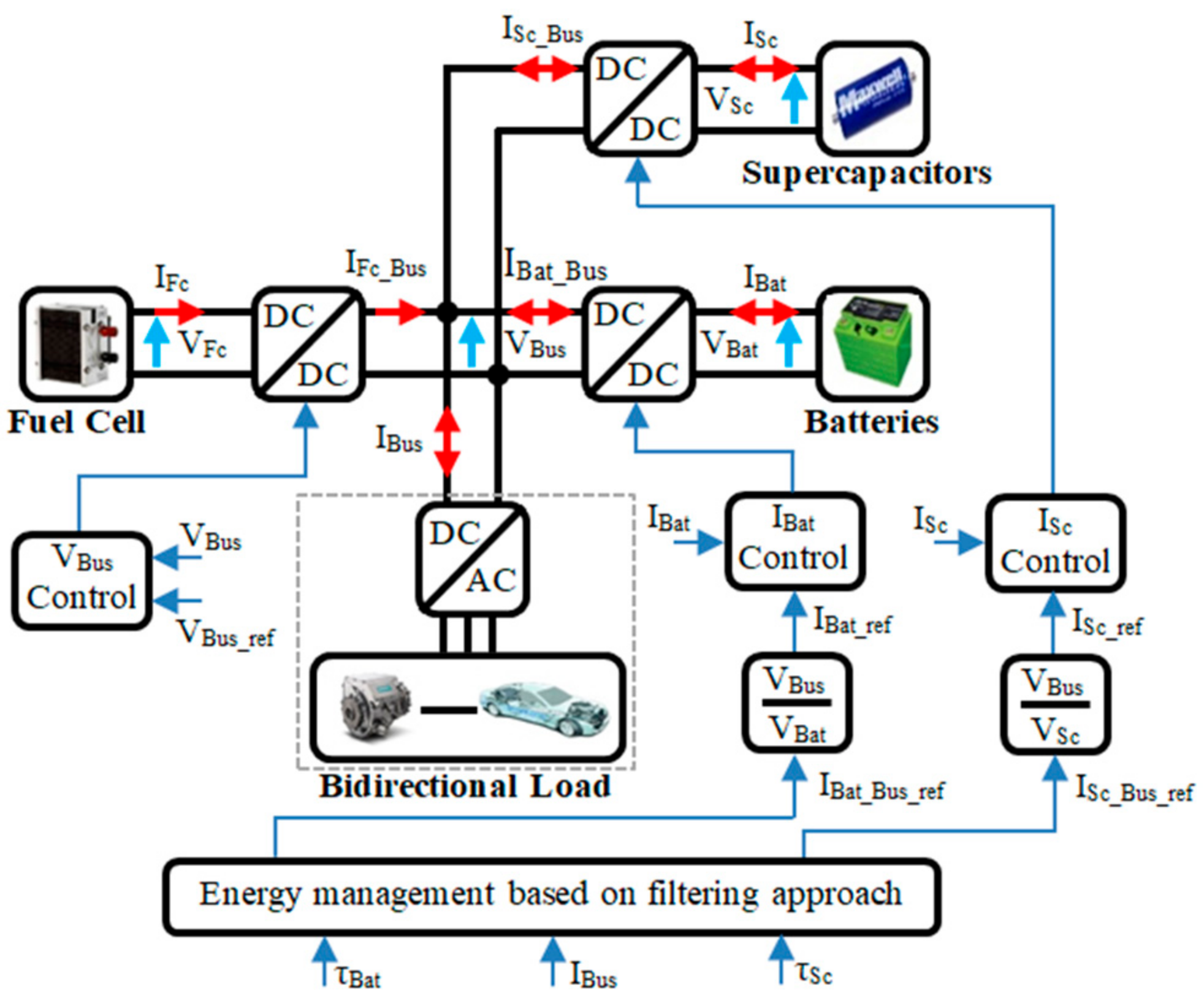
3. Electric Vehicle Energy Management Strategy (EMS)

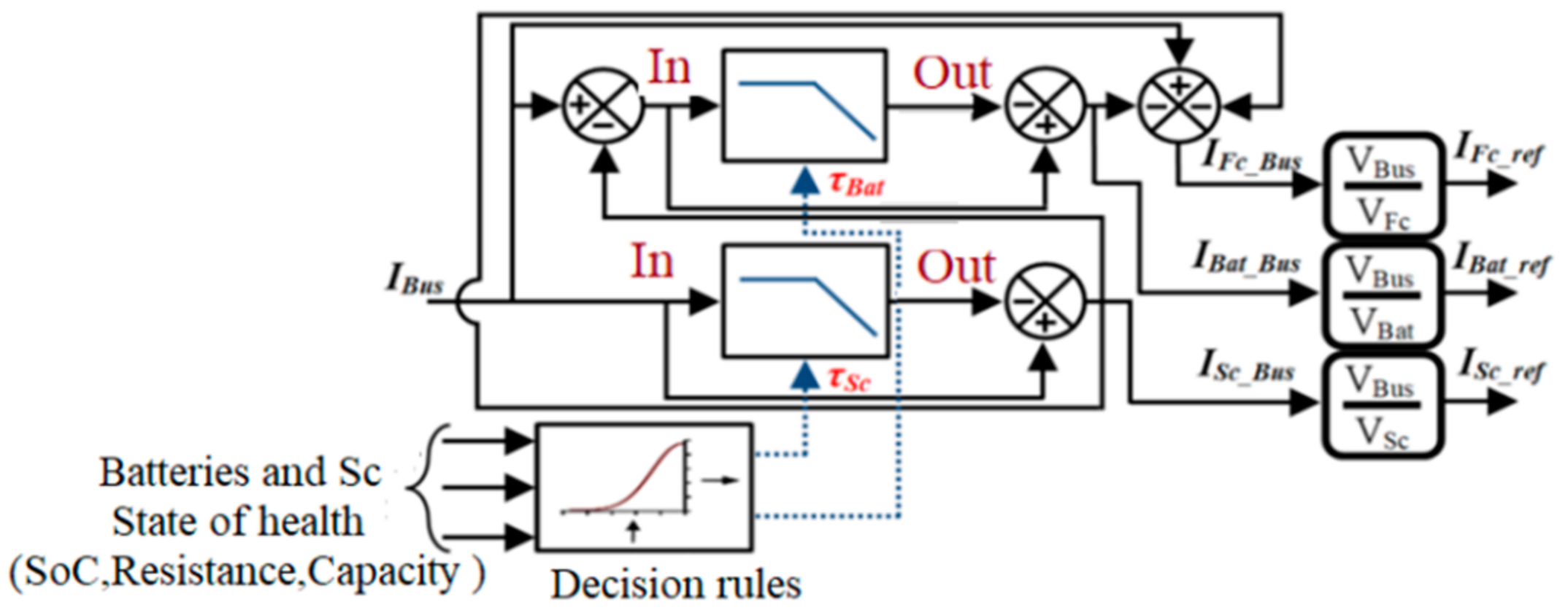
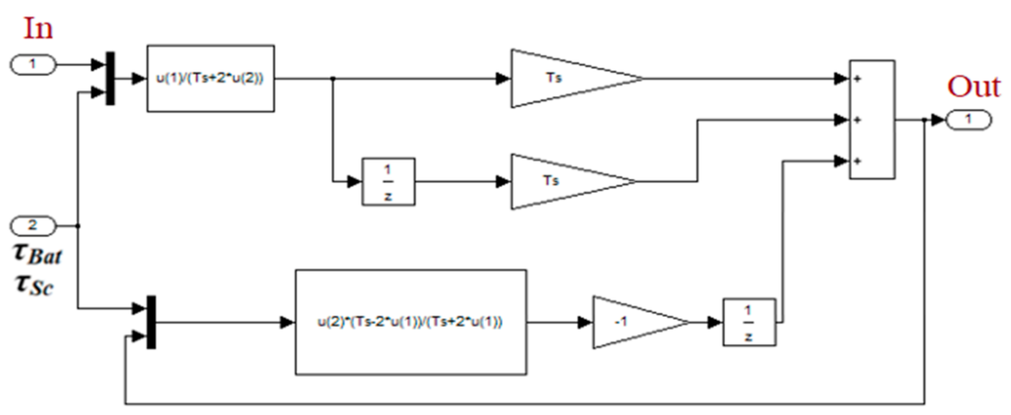
3.1. Filtering Approach for High and Average Frequency Components Extraction from Load’s Current

In EV power supply system, each electric energy storage technology has its own strengths and weaknesses. The EMS developed in this paper focuses on two main properties, namely the specific energy and the specific power. These two features are used to compare the different ESS technologies in terms of electric and dynamic performances [28,29]. Specific power defines the energy source ability to store or retrieve large amounts of energy in short time intervals. In other words, power density defines the energy source ability to respond to the load transient power solicitations, it is measured in W/kg. Specific energy defines the energy autonomy that the ESS can provide for a given application, it is measured in Wh/kg. As shown in Equation (7), the ratio of specific energy over specific power is equivalent to a time constant. A low time constant value indicates that the energy source has good dynamic (fast response) performance. On the other hand, the more the ratio is important, the more the energy source dynamic capability is reduced. Actually there is no ESS that combines satisfactorily a good specific power and a good specific energy. Each ESS has its own frequency range where its functioning is optimal. This indication is very important because it gives an idea on the load solicitations constraints to which the energy source should wisely be subjected to. This is where the idea of EMS based on frequency distribution comes from. This approach is focused on the splitting of the load’s demand into high, average, and low frequency components. Since the Sc dynamic performance is better than that of the batteries and the fuel cells, the high frequency part will be affected to the Sc pack. In terms of dynamic performance, the batteries come in second place after supercapacitors. They will therefore guarantee the medium frequency part of the load requests. Finally, the load low frequency component must be provided by the Fc stack because it is the EV’s main energy source and it has the weakest dynamic response. The initial values of the low-pass filters time constants are calculated as presented in Equation (7). The batteries and the Sc specific energy and power values are available in their datasheets [30,31].

$$\{\begin{array}{l}{\tau }_{sc}\approx \frac{{\rho }_{eSC}}{2\ast \pi \ast {\rho }_{pSC}}=\frac{6\ast 3600\mathrm{W}\mathrm{s}/\mathrm{k}\mathrm{g}}{2\ast \pi \ast 5.9\ast 1000\mathrm{W}/\mathrm{k}\mathrm{g}}=0.58\mathrm{s}\\ {\tau }_{Bat}\approx \frac{{\rho }_{eBat}}{2\ast \pi \ast {\rho }_{pBat}}=\frac{102.24\ast 3600\mathrm{W}\mathrm{s}/\mathrm{k}\mathrm{g}}{2\ast \pi \ast 309.68\mathrm{W}/\mathrm{k}\mathrm{g}}=189\mathrm{s}\end{array}$$

(7)

The originality of EMS is based on the low-pass filters time constants auto-adaptive control concept according to the batteries and Sc state of health. Figure 9 illustrates the principle of the high, average, and low frequency components extraction considering the filters time constants auto-adaptive control concept. In order to adjust the time constants of the filters during simulations and in the real time operations, we proposed a model of the filters so that the value of the time constant becomes an input for the low pass filter as illustrated in Figure 10. This adjustment is necessary to optimize the behavior of the multi-source system when the ESS starts to age. Figure 11 illustrates the overall scheme of the multisource system coordinated EMS and power converters control.

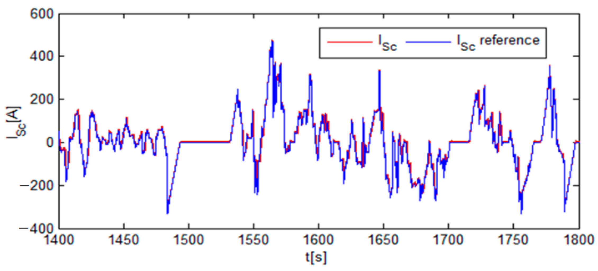
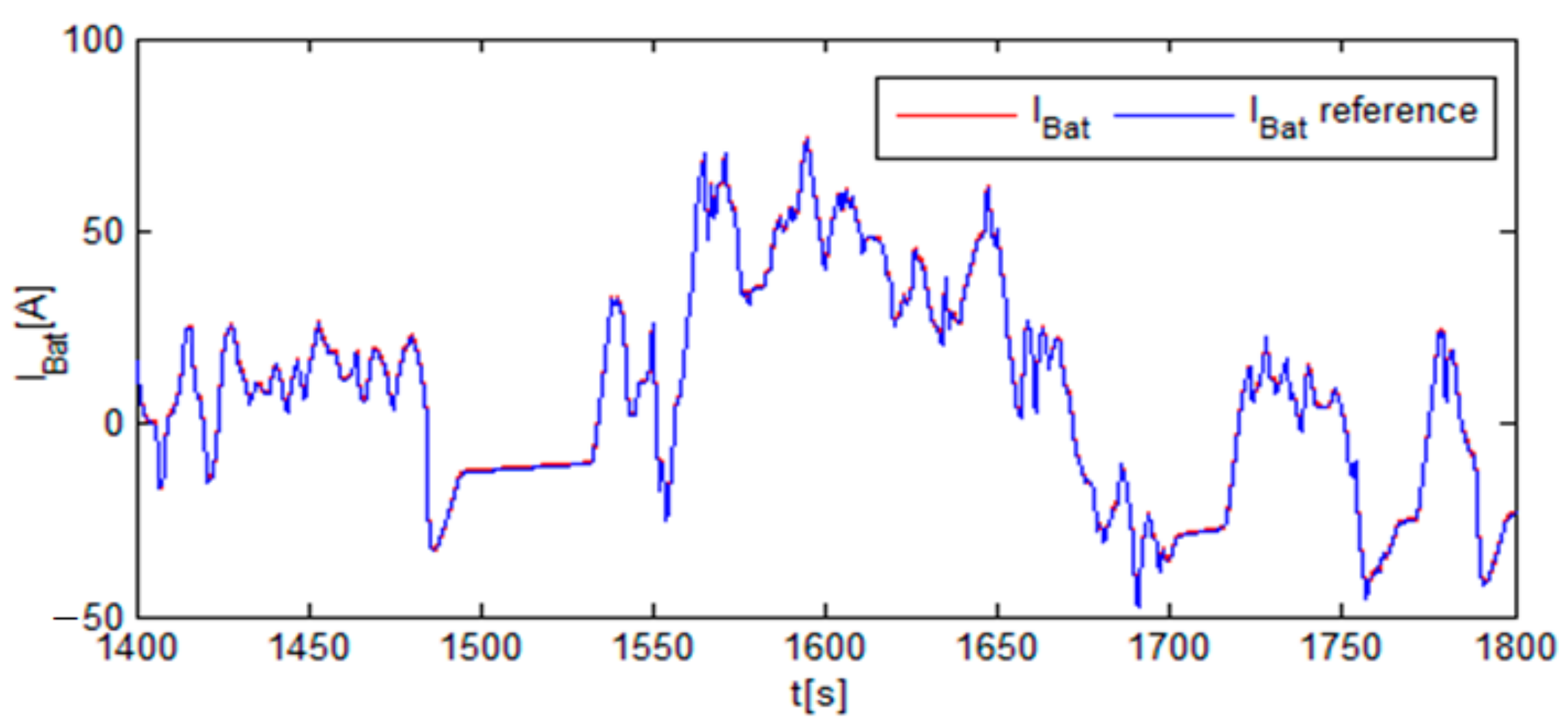
3.2. Supercapacitors and Batteries Current Control

To control the currents of the Sc and the batteries, the model of the buck/boost converter extracted from [32] is used. This model is presented in Equation (8), where k is the current sign and α_Bat/Sc presents the converter duty cycle. The values of k and α_Bat/Sc depend on the converter operation mode. The boost operation corresponds to k = 1 and α_{Bat/Sc_Boost} = 1 − α_Bat/Sc. The buck operation corresponds to k = −1 and α_{Bat/Sc_Buck} = α_Bat/Sc.

$$\{\begin{array}{l}{L}_{Bat/Sc}\ast \frac{d{I}_{Bat/Sc}}{dt}=k\ast \left(V_{Bat/Sc}-{\alpha }_{Bat/Sc}\ast V_{Bus}\right)\\ C_{Bat/Sc}\ast \frac{d{V}_{Bus}}{dt}={\alpha }_{Bat/Sc}\ast I_{Bat/Sc}-I_{Bat/Sc\_Bus}\end{array}$$

(8)

The digital RST controller was chosen to control the batteries and the Sc currents as well as the DC-link voltage. The digital RST controller can independently handle the disturbance rejection and the reference tracking dynamics, taking into account the process delay. The RST controller is based on a robust pole assignment [33]. As presented in Figure 11, the batteries and Sc currents references were obtained from the EMS and power conservation within the buck-boost converters. The three polynomials expressions are given in Equation (9) and their parameters are calculated from Equation (10). In this last equation, T_e presents sampling period, L_Bat and L_Sc are the batteries and Sc currents smoothing inductances, ω_Bat/Sc is the batteries and Sc currents control bandwidth and f_d is the power converters pulse width modulation (PWM) frequency. The batteries’ current dynamic variation was slower than the Sc current one, this was why ω_Sc is chosen as greater than ω_Bat.

$$\{\begin{array}{l}{S}_{Bat/Sc}\left(z^{-1}\right)=1-z^{-1}\\ T_{Bat/Sc}\left(z^{-1}\right)=R_{Bat/Sc}\left(z^{-1}\right)=t_{0Bat/Sc}+t_{1Bat/Sc}\ast z^{-1}\end{array}$$

(9)

$$\{\begin{array}{l}{t}_{0Bat/Sc}=2\ast \left(1-e^{-{\omega }_{Bat/Sc}\ast T_e}\right)\ast \frac{L_{Bat/Sc}}{T_e}\\ t_{1Bat/Sc}=\left(e^{-2\ast {\omega }_{Bat/Sc}\ast T_e}-1\right)\ast \frac{L_{Bat/Sc}}{T_e}\\ {\omega }_{Sc}=2\ast \pi \ast f_d;\hspace{0.17em}\hspace{0.17em}\hspace{0.17em}\hspace{0.17em}\hspace{0.17em}\hspace{0.17em}\hspace{0.17em}\hspace{0.17em}\hspace{0.17em}\hspace{0.17em}\hspace{0.17em}\hspace{0.17em}\hspace{0.17em}{\omega }_{Bat}=\frac{{\omega }_{Sc}}{2}\end{array}$$

(10)

The batteries and Sc currents control loops are illustrated in Figure 12, the duty cycle value for buck and boost operations are achieved from Equation (11).

$$\{\begin{array}{l}{\alpha }_{Buck\_Bat/Sc}=\frac{V_{Bat/Sc}+V_{LBat/Sc}}{V_{Bus}}\\ {\alpha }_{Boost\_Bat/Sc}=1-\frac{V_{Bat/Sc}-V_{LBat/Sc}}{V_{Bus}}\end{array}\hspace{0.17em}$$

(11)

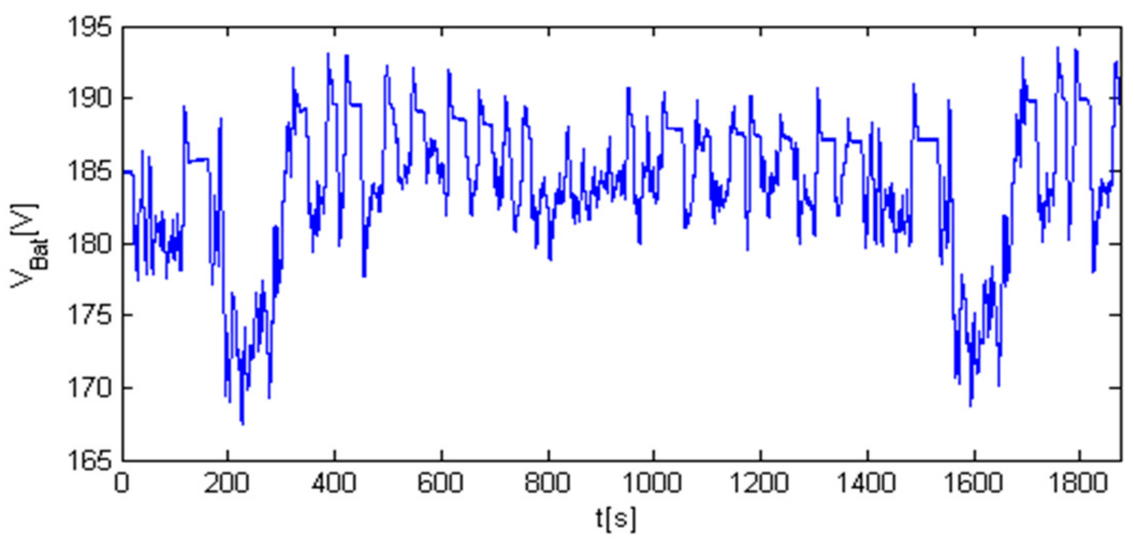
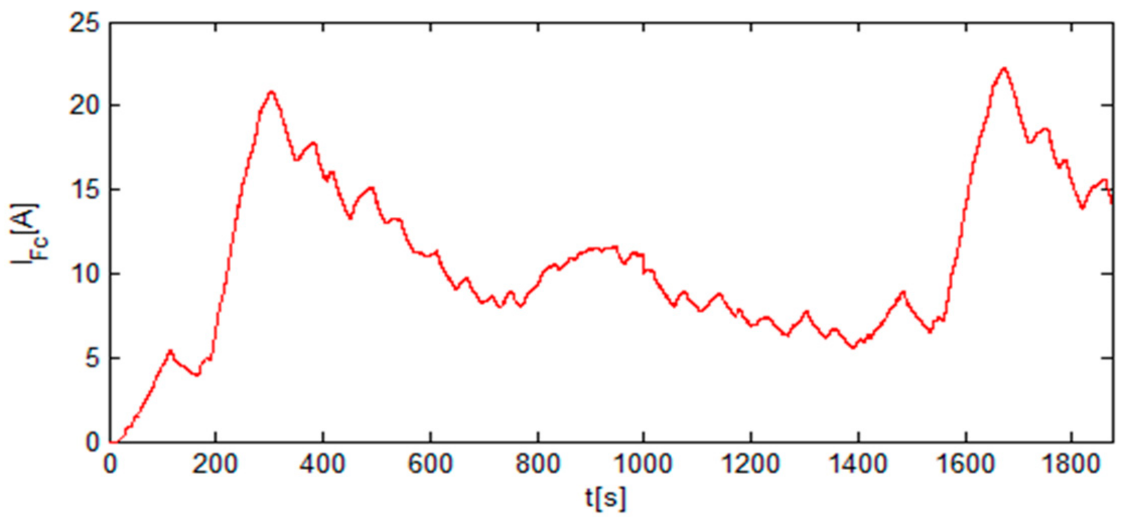
3.3. DC-Link Voltage Management

The three channels’ interleaved boost converter enabled to reduce the power conduction losses. Thanks to the current sharing between the three channels, the global current ripples can be reduced compared to classic boost converter. About control issue, three channels PWM signals will be used with phase shifted of 120°. Equation (12) presents the converter model, where α_Fc1, α_Fc2, α_Fc3 present the converter duty cycles. This model was used for system behavior simulations.

$$\{\begin{array}{l}{L}_1\ast \frac{d{I}_{L1}}{dt}=V_{Fc}-\left(1-{\alpha }_{Fc1}\right)\ast V_{Bus}\\ L_2\ast \frac{d{I}_{L2}}{dt}=V_{Fc}-\left(1-{\alpha }_{Fc2}\right)\ast V_{Bus}\\ L_3\ast \frac{d{I}_{L3}}{dt}=V_{Fc}-\left(1-{\alpha }_{Fc3}\right)\ast V_{Bus}\\ I_{Fc}=I_{L1}+I_{L2}+I_{L3}\end{array}$$

(12)

The DC-link voltage control was decoupled from the batteries and Sc current control loops. In most cases, controlling the DC-link voltage requires a cascade control loop [4]. In this paper, a single voltage control loop was used, which enabled to directly affect to Fc the low frequency part of the load solicitations. The used polynomial RST controllers are given in Equation (13), and their parameters are calculated using Equation (14), where C_Bat, C_Sc, and C_Fc are the output capacitors of the converters linked respectively to the batteries, Sc, and the Fc. C_T presents the total capacitor in DC-link and ω_Fc is the voltage control bandwidth. The duty cycle α_{Boost_Fc} has the same expression as α_{Boost_Bat/Sc}. DC-link voltage management principle is illustrated in Figure 13.

$$\{\begin{array}{l}{S}_{Fc}\left(z^{-1}\right)=1-z^{-1}\\ T_{Fc}\left(z^{-1}\right)=R_{Fc}\left(z^{-1}\right)=t_{0Fc}+t_{1Fc}\ast z^{-1}\end{array}$$

(13)

$$\{\begin{array}{l}{t}_{0Fc}=2\ast \left(1-e^{-{\omega }_{Fc}\ast T_e}\right)\ast \frac{C_T}{T_e}\\ t_{1Fc}=\left(e^{-2\ast {\omega }_{Fc}\ast T_e}-1\right)\ast \frac{C_T}{T_e}\\ C_T=C_{Fc}+C_{Bat}+C_{Sc}+C_{Bus};\hspace{0.17em}\hspace{0.17em}\hspace{0.17em}\hspace{0.17em}{\omega }_{Fc}=\frac{{\omega }_{Sc}}{100}\end{array}$$

(14)

Table 4. System control parameters.

Description	Symbol	Parameters
DC-link capacitance ISc and IBat smoothing inductances Sc current control parameters	CSc = CBat = CFc = CBus LSc = LBat t0Sc; t1Sc	3.3 mF 12 mH 110.27; 59.60
Battery’s current control parameters	t0Bat; t1Bat	85.84; 55.13
DC-link voltage control parameters	t0Fc; t1Fc	3.27; 3.23
PWM frequency	fd	2 kHz

contains all necessary parameters to manage the DC-link voltage as well as the powers (currents) of the batteries and Sc.

4. Simulations and Experimental Verifications

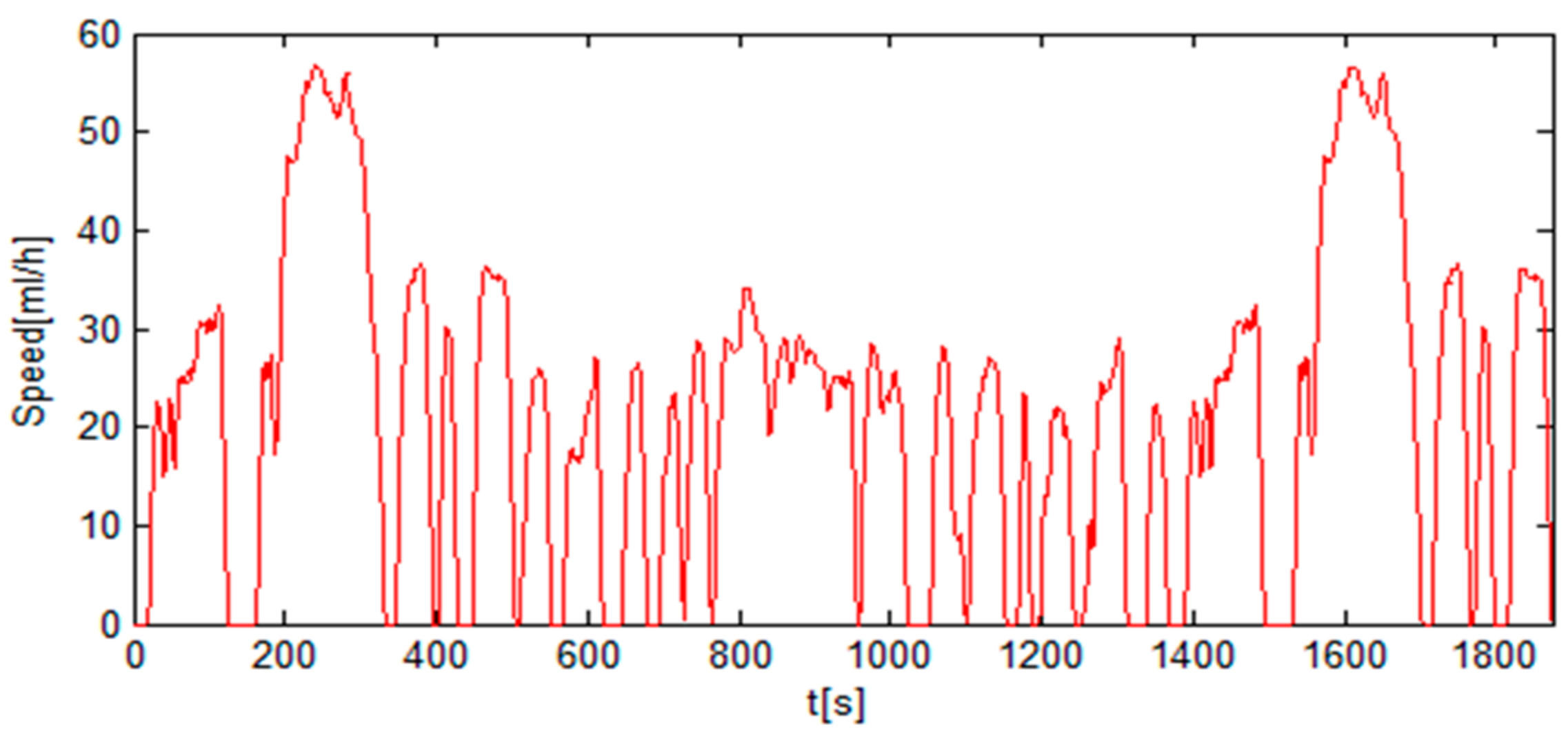
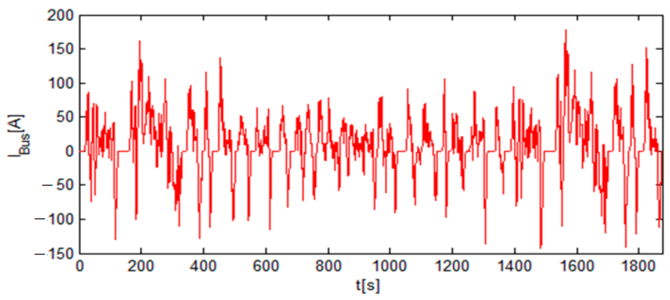
4.1. Simulation Conditions

The used speed profile is based on the US driving cycle illustrated in Figure 14. This driving cycle was chosen because it reflects relatively well the speed levels achieved by the majority of drivers. It is spread over a distance of 17.77 km for a duration equal to 1874 s with a middling speed of 34 km/h. The power profile was obtained from the real dimensions of the Volkswagen e-UP electric car with a rated power of 60 kW and a DC-link voltage equal to 374 V [34].

This vehicle is considered as an example for EV behavior simulations. The rated parameters of Volkswagen E-Up electric car and more technical information can be found in [34]. In EV applications, the DC-link voltage value is generally constant. However, to show the efficiency of the voltage management, the set points imposed to DC-link voltage are, respectively, 374 and 340 V. The driving cycle curve presents three different situations: the first case corresponds to accelerations where the Sc or batteries will be solicited depending on the nature of the vehicle’s demand (fast or slow acceleration). The second case corresponds to decelerations. In this case, the Sc or batteries will recover the energy from the traction chain depending on the deceleration nature (strong braking or slow deceleration). The third case corresponds to a constant or zero speed. In this case, the Sc and batteries are not solicited, the Fc provides the energy required by the load.

4.2. Simulation Results

The energy sources contributions and EV solicitations are presented in current since the DC-link voltage was generally constant. The load’s current was obtained by dividing the product of traction motor speed and torque (load power) by the DC-link voltage. The load’s current profile I_Bus is presented in Figure 15. This current illustrates the EV instantaneous demand during the driving cycle, it therefore contains the no fluctuating parts in case of a constant speed (highway zone) and the fluctuating requests in case of rapid accelerations, decelerations, and braking operations (urban zone). Figure 16 shows the Sc pack current. A zoom on this current shape is presented in Figure 17, where the Sc current is close to its reference. This current corresponds to the high frequency part of the load’s current, and it reflects the load dynamic behavior that corresponds to the EV acceleration, deceleration, and braking. The Sc pack terminal voltage is shown in Figure 18. The shape of this curve shows three different states. The first state corresponds to accelerations. In this case, the EMS through the low-pass filters assigns the high frequency component to the Sc pack, which causes its voltage to decrease. The second state corresponds to a strong deceleration or braking modes. In this case, the Sc pack recovers energy, which causes the voltage to increase. The third state corresponds to Sc pack constant voltage. In this case, the load demand is not fluctuating, therefore the EMS does not solicit the Sc pack because the vehicle speed is constant or equal to zero. Figure 19 illustrates the batteries’ current, which represents the load medium frequency component. The zoom section of the batteries current is plotted in Figure 20, where I_Bat is close to its reference. Batteries voltage is shown in Figure 21. This curve presents almost the same fluctuations as V_Sc, but with different levels of variations. In comparison with the batteries’ module, the Sc pack is subject to faster and higher current magnitude. Nevertheless, the batteries’ module voltage and the Sc pack ones present the same situations. Figure 22 shows the low frequency part of the vehicle request provided by the Fc stack. This current varies slowly compared to the batteries and Sc currents. Fc voltage is shown in Figure 23. Apart from the first variation, which corresponds to a voltage drop due to Fc voltage activation, V_Fc does not change significantly, which means that the Fc is not solicited during the EV transient states. DC-link voltage reference is slightly changed to show the voltage control efficiency as shown in Figure 24, where DC-link voltage is close to the set point. Based on the simulation results, the implemented RST controller and the EMS are satisfactory. The load’s current fluctuations are compensated by the batteries and Sc, therefore the Fc is protected because it only supplies the low frequency component adapted to it dynamic capability.

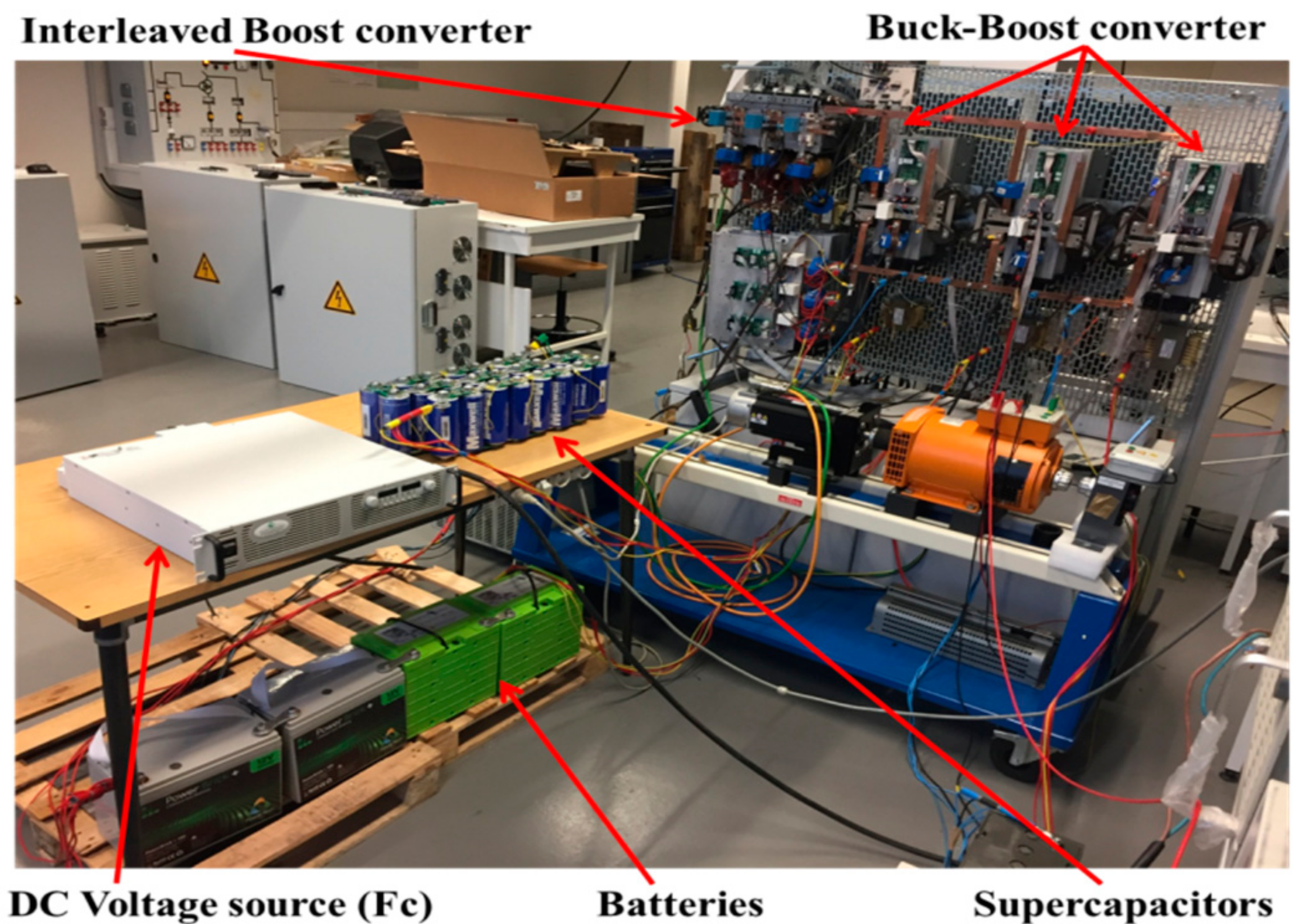
4.3. Experimental Tests Conditions

The experimental tests were performed via a reduced-scale test bench according to the available equipment in the laboratory. The reduction factor was 50 and the test bench is illustrated in Figure 25. It contained a Sc pack based on 24 cells of BoostCap (2.7 V/3000F) in series, a LiFePO₄ batteries module of 4 batteries (12 V/100Ah) in series. Sc pack and the batteries module are connected to the DC-link via two buck-boost converters in order to manage, respectively, the high frequency part and the medium frequency part extracted from the load’s current. The fuel cell was emulated using a programmable DC voltage source to manage the DC-link voltage via three channels interleaved boost converters and to compensate the load current low frequency component. The maximum voltage of the Fc emulator was fixed to 39.5 V. The vehicle power demand was emulated using a bidirectional controlled DC load. DC-link voltage reference was initially fixed to 100 V in order to decrease the number of Sc and batteries needed to perform the EMS experimental verifications. In order to verify the performance of the DC-link voltage control, the voltage reference was changed to 90 V during experimental tests. The control algorithm was implemented in dSPACE environment using Matlab/Simulink and Control Desk software.

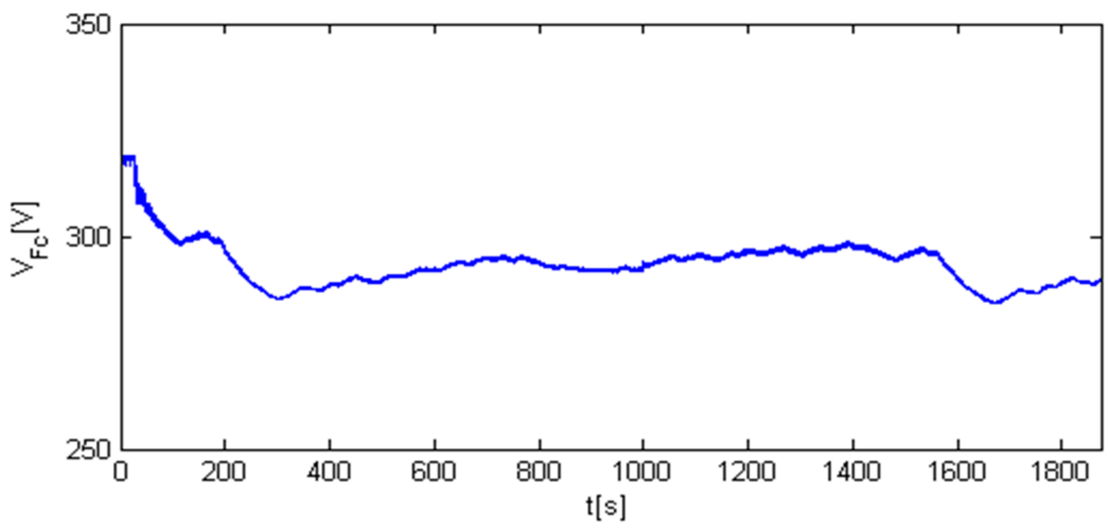
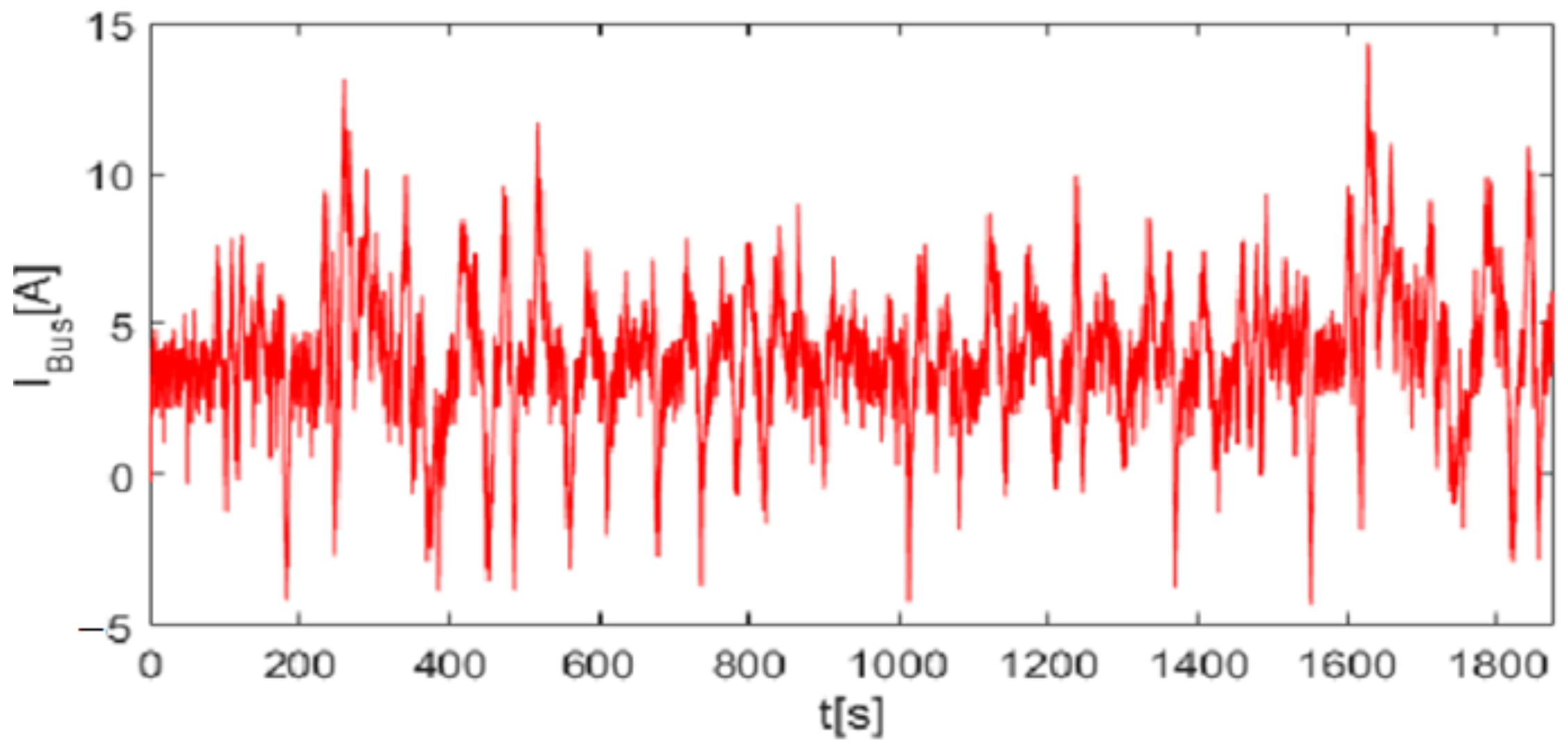
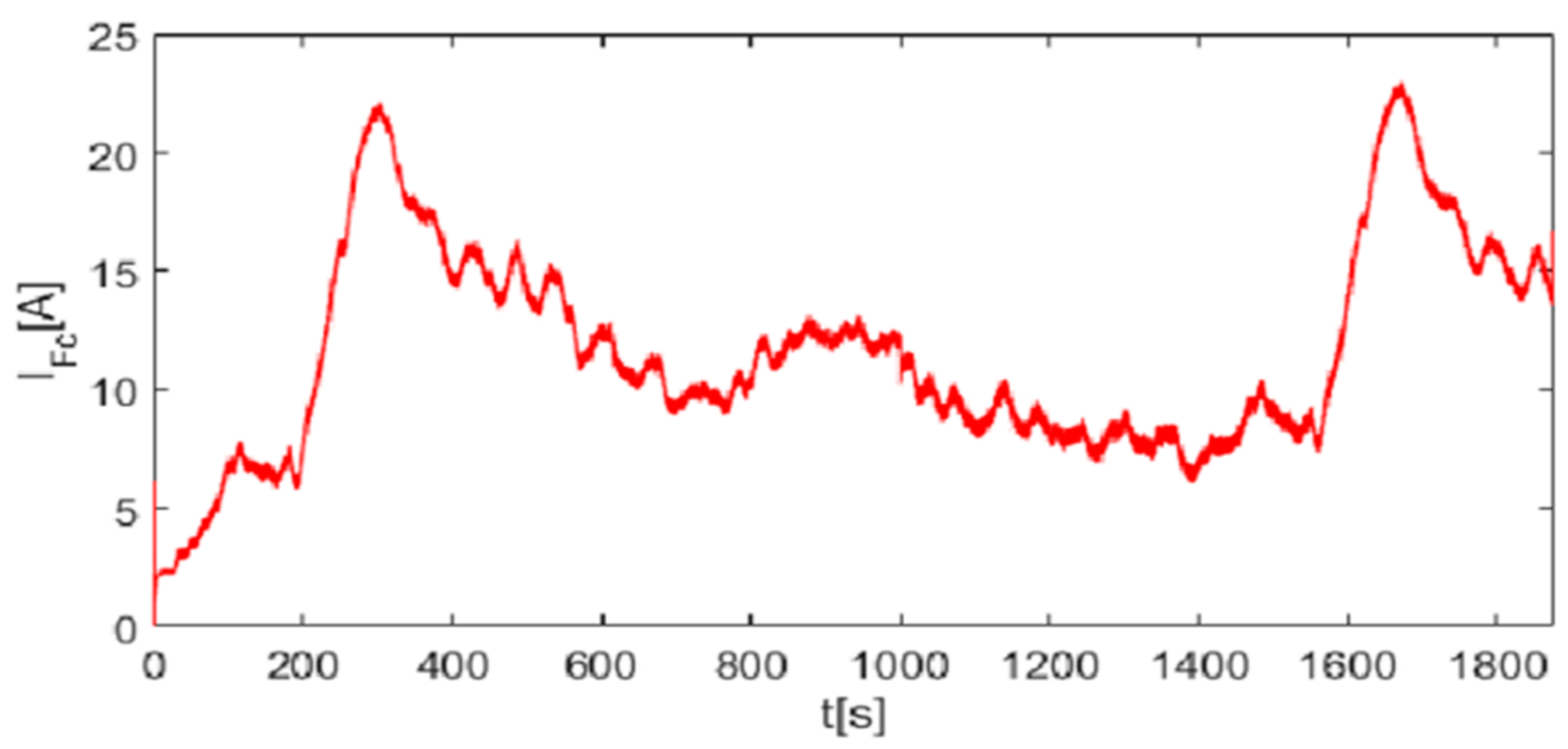
4.4. Experimental Results

Figure 26 illustrates the load current shared between the Sc, the batteries, and Fc considering to the dynamic performances of these sources. This figure has the same fluctuations compared to simulation curve plotted in Figure 15, however the magnitudes were different due to the power scale disparity between simulation environment and experimental test bench. Figure 27 and Figure 28 illustrate respectively the Fc stack current and terminal voltage. Figure 27 shows that the Fc delivers the low frequency part of the load current, which presents more fluctuations and more current peak with a no null initial condition compared to the simulations result shown in Figure 22. These contrarieties were essentially due to the difference of the dynamic characteristics between the DC source and the Fc model. Figure 28 shows that the terminal voltage of the Fc decreased according to current magnitude increasing. This figure shows a similar waveform just as the simulation result presented in Figure 23, but with more fluctuations owing to the DC-source dynamic characteristics limitations (low magnitude due to the experimental tests reduced scale). Figure 29 and Figure 30 show, respectively, the batteries current control result and its zoom. The batteries module compensated the medium frequency part of the load power demand as illustrated in Figure 29. This curve was obtained with a road flat condition, which justified the waveform shape difference when compared to the simulation presented in Figure 19. In addition, the simulation and experimental current results were not the same in terms of magnitudes as the power scale was different for both validations. The zoom of the measured current I_Bat and its reference were close, as presented in Figure 30. The measured voltage across the batteries module, presented in Figure 31, did not change significantly compared to the simulation result shown in Figure 21, this was due to the low current request according to the EMS and the test bench high capacity batteries (100Ah). Figure 31 shows three variations cases: the first case corresponds to the batteries charge, this situation corresponds to the energy recovery from EV braking operations and decelerating ones. The second case corresponds to V_Bat decrease due to the battery discharge. This state corresponds to a power demand during the EV acceleration operations. The third case corresponds to a non-fluctuating load demand, where the Sc and batteries are not solicited. Figure 32 and Figure 33 present, respectively, the Sc pack current and a zoom section of this last one, where the measured current is close to its reference. Figure 32 has the same fluctuations compared to simulation result in Figure 16, but the magnitudes are not the same due to difference of the power scale. Figure 32 shows that the high frequency part of the load demand was well compensated by the Sc pack and I_Sc variations were significant in comparison to Fc current (Figure 27) and the batteries ones (Figure 29). Sc pack terminal voltage, shown in Figure 34, presents three cases of variations similar to V_Bat, but with high magnitude and significant frequencies. The terminal Sc pack voltage presented in Figure 34 is different from the simulation (Figure 18) due to reduced power scale requirement that necessitate the Sc current magnitude adjustment in the goal to respect the minimum and maximum voltage limits. The DC-link measured and set point voltages are plotted in Figure 35. These curves show a very small gap between the measurement and the reference.

As reported in the experimental and simulations verifications sections, the supercapacitors pack simulation result, presented in Figure 16 and experimental result shown in Figure 32, contained the high frequency part of the load demand. The same goes with the batteries contribution results, where the medium frequency part is presented in Figure 19 and Figure 29. Finally, the Fc contribution results presented in Figure 22 and Figure 27 represent the low frequency part of the load requests. According to the experimental curves discussion presented in this section, the experimental results approved the validity of the simulations presented in the previous section.

5. Conclusions

In this paper, EMS based on the EV power demand distribution is presented. This distribution of energy and power requested by the EV traction chain is done taking into account the onboard sources time response. Fc ensures the vehicle’s energy production, while the Sc and batteries assist the main energy source during transient operations due to acceleration, deceleration and braking operations. In addition, a new model of the Sc taking into account electric and thermal stresses is proposed. According to the results obtained through behavioral simulation and experimental tests, the adopted EMS seemed to be very effective for a multisource system. On one hand, it took into account the energy sources capabilities by reducing the load’s current fluctuations impact on the fuel cell. On the other hand, it exploited the performances of energy sources with high specific power and great dynamic capabilities. In other words, the contribution of the Sc pack handled the majority of the fluctuations from the load’s current. The batteries’ contribution contained some fluctuations, but with lower frequencies and amplitude in comparison to those ensured by the Sc pack. Finally, the fuel cell provided only the low frequency component adapted to its dynamic performance. Regarding the perspectives of this study, the actual energy management doesn’t consider the long-time aging impact on the energy sources SoC and SoH. In fact, the real time energy management requires several months of tests to obtain a significant aging for an energy storage device. Future research works will be dedicated to this new challenge.

References

1. Abdelrahmana, S.; Attiaa, Y.; Woronowiczb, K.; Youssef, M.Z. Hybrid Fuel Cell/Battery Rail Car: A Feasibility Study. IEEE Trans Transp. Electrif. 2016, 2, 493–503. [Google Scholar] [CrossRef]
2. Yin, H.; Zhou, W.; Li, M.; Ma, C.; Zhao, C. An Adaptive Fuzzy Logic-Based Energy Management Strategy on Battery/Ultracapacitor Hybrid Electric Vehicles. IEEE Trans. Transp. Electrif. 2016, 2, 300–311. [Google Scholar] [CrossRef]
3. Shen, J.; Khaligh, A. A Supervisory Energy Management Control Strategy in a Battery/Ultracapacitor Hybrid Energy Storage System. IEEE Trans Transp. Electrif. 2015, 1, 223–231. [Google Scholar] [CrossRef]
4. Itani, K.; De Bernardinis, A.; Jammal, A.; Oueidat, M. Extreme conditions regenerative braking modeling, control and simulation of a hybrid energy storage system for an electric vehicle. IEEE Trans Transp. Electrif. 2016, 2, 465–479. [Google Scholar] [CrossRef]
5. Snoussi, J.; Ben Elghali, S.; Benbouzid, M.; Mimouni, M.F. Optimal Sizing of Energy Storage Systems Using Frequency-Separation-Based Energy Management for Fuel Cell Hybrid Electric Vehicles. IEEE Trans. Veh. Technol. 2018, 67, 9337–9346. [Google Scholar] [CrossRef]
6. Han, Y.; Li, Q.; Wang, T.; Chen, W.; Ma, L. Multisource Coordination Energy Management Strategy Based on SOC Consensus for a PEMFC–Battery–Supercapacitor Hybrid Tramway. IEEE Trans. Veh. Technol. 2017, 67, 296–305. [Google Scholar] [CrossRef]
7. Huang, Y.; Wang, H.; Khajepour, A.; Li, B.; Ji, J.; Zhao, K.; Hu, C. A review of power management strategies and component sizing methods for hybrid vehicles. Renew. Sustain. Energy Rev. 2018, 96, 132–144. [Google Scholar] [CrossRef]
8. Hossain, M.; Rahim, N.; Selvaraj, J.A. Recent progress and development on power DC-DC converter topology, control, design and applications: A review. Renew. Sustain. Energy Rev. 2018, 81, 205–230. [Google Scholar] [CrossRef]
9. Sorlei, I.-S.; Bizon, N.; Thounthong, P.; Varlam, M.; Carcadea, E.; Culcer, M.; Iliescu, M.; Raceanu, M. Fuel Cell Electric Vehicles—A Brief Review of Current Topologies and Energy Management Strategies. Energies 2021, 14, 252. [Google Scholar] [CrossRef]
10. Odeim, F.; Roes, J.; Heinzel, A. Power Management Optimization of an Experimental Fuel Cell/Battery/Supercapacitor Hybrid System. Energies 2015, 8, 6302–6327. [Google Scholar] [CrossRef] [Green Version]
11. Sampietro, J.L.; Puig, V.; Costa-Castelló, R. Optimal Sizing of Storage Elements for a Vehicle Based on Fuel Cells, Supercapacitors, and Batteries. Energies 2019, 12, 925. [Google Scholar] [CrossRef] [Green Version]
12. Gherairi, S. Hybrid Electric Vehicle: Design and Control of a Hybrid System (Fuel Cell/Battery/Ultra-Capacitor) Supplied by Hydrogen. Energies 2019, 12, 1272. [Google Scholar] [CrossRef] [Green Version]
13. Nassef, A.M.; Fathy, A.; Rezk, H. An Effective Energy Management Strategy Based on Mine-Blast Optimization Technique Applied to Hybrid PEMFC/Supercapacitor/Batteries System. Energies 2019, 12, 3796. [Google Scholar] [CrossRef] [Green Version]
14. Do, T.C.; Truong, H.V.A.; Dao, H.V.; Ho, C.M.; To, X.D.; Dang, T.D.; Ahn, K.K. Energy Management Strategy of a PEM Fuel Cell Excavator with a Supercapacitor/Battery Hybrid Power Source. Energies 2019, 12, 4362. [Google Scholar] [CrossRef] [Green Version]
15. Hussain, S.; Ali, M.U.; Park, G.-S.; Nengroo, S.H.; Khan, M.A.; Kim, H.-J. A Real-Time Bi-Adaptive Controller-Based Energy Management System for Battery–Supercapacitor Hybrid Electric Vehicles. Energies 2019, 12, 4662. [Google Scholar] [CrossRef] [Green Version]
16. Nazir, M.S.; Ahmad, I.; Khan, M.J.; Ayaz, Y.; Armghan, H. Adaptive Control of Fuel Cell and Supercapacitor Based Hybrid Electric Vehicles. Energies 2020, 13, 5587. [Google Scholar] [CrossRef]
17. Han, J.; Charpentier, J.-F.; Tang, T. An Energy Management System of a Fuel Cell/Battery Hybrid Boat. Energies 2014, 7, 2799–2820. [Google Scholar] [CrossRef] [Green Version]
18. Liu, J.; Li, Q.; Chen, W.; Yan, Y.; Wang, X. A Fast Fault Diagnosis Method of the PEMFC System Based on Extreme Learning Machine and Dempster–Shafer Evidence Theory. IEEE Trans. Transp. Electrif. 2019, 5, 271–284. [Google Scholar] [CrossRef]
19. Liang, M.; Liu, Y.; Xiao, B.; Yang, S.; Wang, Z.; Han, H. An analytical model for the transverse permeability of gas diffusion layer with electrical double layer effects in proton exchange membrane fuel cells. Int. J. Hydrogen Energy 2018, 43, 17880–17888. [Google Scholar] [CrossRef]
20. Wang, Y.X.; Ou, K.; Kim, Y.B. Modeling and experimental validation of hybrid proton exchange membrane fuel cell/battery system for power management control. Int. J. Hydrogen Energy 2015, 40, 11713–11721. [Google Scholar] [CrossRef]
21. Cao, Y.; Kroeze, R.C.; Krein, P.T. Multi-timescale Parametric Electrical Battery Model for Use in Dynamic Electric Vehicle Simulations. IEEE Trans. Transp. Electrif. 2016, 2, 432–442. [Google Scholar] [CrossRef]
22. Bellache, K.; Camara, M.B.; Dakyo, B.; Sridhar, R. Aging characterization of lithium iron phosphate batteries considering temperature and direct current undulations as degrading factors. IEEE Trans. Ind. Electron. 2020, 1. [Google Scholar] [CrossRef]
23. El Mejdoubi, A.; Chaoui, H.; Gualous, H.; Sabor, J. Online Parameter Identification for Supercapacitor State-of-Health Diagnosis for Vehicular Applications. IEEE Trans. Power Electron. 2017, 32, 9355–9363. [Google Scholar] [CrossRef]
24. Ahmad, H.; Wan, W.Y.; Isa, D. Modeling the Ageing Effect of Cycling Using a Supercapacitor-Module Under High Temperature with Electrochemical Impedance Spectroscopy Test. IEEE Trans. Reliab. 2018, 68, 109–121. [Google Scholar] [CrossRef]
25. Liu, W.; Song, Y.; Liao, H.; Li, H.; Zhang, X.; Jiao, Y.; Peng, J.; Huang, Z. Distributed Voltage Equalization Design for Supercapacitors Using State Observer. IEEE Trans. Ind. Appl. 2018, 55, 620–630. [Google Scholar] [CrossRef]
26. Murray, D.B.; Hayes, J.G. Cycle Testing of Supercapacitors for Long-Life Robust Applications. IEEE Trans. Power Electron. 2015, 30, 2505–2516. [Google Scholar] [CrossRef]
27. Bellache, K.; Camara, M.B.; Dakyo, B.; Brayima, D. Supercapacitors Characterization and Modeling Using Combined Electro-Thermal Stress Approach Batteries. IEEE Trans. Ind. Appl. 2018, 55, 1817–1827. [Google Scholar] [CrossRef]
28. Camara, M.B.; Gualous, H.; Gustin, F.; Berthon, A.; Dakyo, B. DC/DC Converter Design for Supercapacitor and Battery Power Management in Hybrid Vehicle Applications—Polynomial Control Strategy. IEEE Trans. Ind. Electron. 2010, 57, 587–597. [Google Scholar] [CrossRef]
29. Snoussi, J.; Ben Elghali, S.; Benbouzid, M.; Mimouni, M.F. Auto-Adaptive Filtering-Based Energy Management Strategy for Fuel Cell Hybrid Electric Vehicles. Energies 2018, 11, 2118. [Google Scholar] [CrossRef] [Green Version]
30. Datasheet Maxwell Technologies, K2 Ultracapacitors-2.7V Series. Available online: https://www.maxwell.com/images/documents/k2series_ds_10153704.pdf (accessed on 15 April 2021).
31. GWL Power, Technical specification, Winston-LFP100AHA TALL Cell. Available online: https://files.gwl.eu/inc/_doc/attach/StoItem/7705/ThunderSky-Winston-LIFEPO4-100Ah-TALL-Datasheet.pdf (accessed on 15 April 2021).
32. Oukkacha, I.; Camara, M.B.; Dakyo, B. Energy Management in Electric Vehicle based on Frequency sharing approach, using Fuel cells, Lithium batteries and Supercapacitors. In Proceedings of the 2018 7th International Conference on Renewable Energy Research and Applications (ICRERA), Paris, France, 14–17 October 2018; pp. 986–992. [Google Scholar] [CrossRef]
33. Khanchoul, M.; Hilairet, M. Design and comparison of different RST controllers for PMSM control. In Proceedings of the IECON 2011–37th Annual Conference of the IEEE Industrial Electronics Society, Melbourne, VIC, Australia, 7–10 November 2011; pp. 1795–1800. [Google Scholar] [CrossRef]
34. Technical Specifications for the e-Up Volkswagen Electric Car, 2017 Model. Available online: https://ev-database.org/car/1081/Volkswagen-e-Up (accessed on 15 April 2021).
Figure 1. Electric vehicle (EV) system configuration.
Energies 14 02251 g001
Figure 2. Electric behavioral model of the LiFePO4 batteries.
Energies 14 02251 g002
Figure 3. Supercapacitors (Sc) resistance as function of the temperature and DC-current ripples frequency Fr in [Hz] for 500 cycles.
Energies 14 02251 g003
Figure 4. Sc capacitance as function of temperature and DC-current ripples frequency Fr in [Hz] for 500 cycles.
Energies 14 02251 g004
Figure 5. Behavior model of the Sc pack.
Energies 14 02251 g005
Figure 6. DC-current profile based on FTP-75 (US Federal Test Procedure 75).
Energies 14 02251 g006
Figure 7. Sc cell terminal voltages obtained from experimental and simulations tests.
Energies 14 02251 g007
Figure 8. Sc parameter variations when temperature varies from 10 to 45 °C.
Energies 14 02251 g008
Figure 9. Principle of high, average, and low components extraction from the load’s current.
Energies 14 02251 g009
Figure 10. Principle of low-pass filters time constants variation in real time conditions.
Energies 14 02251 g010
Figure 11. Overall scheme of the EV energy management strategy and power converters control.
Energies 14 02251 g011
Figure 12. Batteries and Sc currents control strategy.
Energies 14 02251 g012
Figure 13. DC-link voltage control loop.
Energies 14 02251 g013
Figure 14. Federal Test Procedure (FTP-75) driving cycle.
Energies 14 02251 g014
Figure 15. Load current profile.
Energies 14 02251 g015
Figure 16. Current of the Sc corresponding to high frequency component.
Energies 14 02251 g016
Figure 17. Zoom on the Sc current control result.
Energies 14 02251 g017
Figure 18. Sc pack terminal voltage.
Energies 14 02251 g018
Figure 19. Battery current corresponding to medium frequency component.
Energies 14 02251 g019
Figure 20. Zoom on the batteries current control result.
Energies 14 02251 g020
Figure 21. Batteries module terminal voltage.
Energies 14 02251 g021
Figure 22. Fuel cell current corresponding to low frequency component.
Energies 14 02251 g022
Figure 23. Fuel cell stack terminal voltage.
Energies 14 02251 g023
Figure 24. DC-link voltage control result.
Energies 14 02251 g024
Figure 25. Reduced scale test bench.
Energies 14 02251 g025
Figure 26. Bidirectional load current.
Energies 14 02251 g026
Figure 27. Current of the fuel cell.
Energies 14 02251 g027
Figure 28. Terminal voltage of the fuel cell.
Energies 14 02251 g028
Figure 29. Battery current control result.
Energies 14 02251 g029
Figure 30. Zoom on the battery current control result.
Energies 14 02251 g030
Figure 31. Battery terminal voltage.
Energies 14 02251 g031
Figure 32. Sc current control result.
Energies 14 02251 g032
Figure 33. Zoom on the Sc current control result.
Energies 14 02251 g033
Figure 34. Supercapacitor module terminal voltage.
Energies 14 02251 g034
Figure 35. DC-link voltage control result.
Energies 14 02251 g035