Simulative Investigation of Thermal Capacity Analysis Methods for Metallic Latent Thermal Energy Storage Systems

Abstract

Latent heat storage systems are a promising technology for storing and providing thermal energy with low volume, mass and cost requirements, especially when operated at high temperatures. Metallic phase change materials are particularly advantageous for high thermal input and output, which is especially important for mobile applications. When designing a storage system, it is essential to have precise knowledge about the potential storage capacity. However, the system’s storage capacity is typically calculated from material properties determined at lab scale, although systemic boundary conditions can have a considerable influence. Systemic influences can result from thermal and reactive interfaces or from the storage design. In order to consider these influences, we propose three calorimetric procedures to thermally analyse high-temperature metallic latent energy storage systems at an application scale. We examined the procedures in a transient simulation environment, monitoring the storage capacity of the system. The procedure, based on adiabatic conditions, shows the least deviation from the simulation input parameters, but is limited to the heating process of the storage. Discharging the storage can be represented by isoperibolic conditions with controlled heat exchange. The precision of the procedures depends on the evaluation routine, the calibration routine, the heat extraction rate and the thermal inertia of the test bench.

1. Introduction

As the electrification of vehicles increases, the challenge of ensuring thermal management without excess waste heat from combustion gains importance [1,2,3]. Utilising the traction battery to cover heating demand leads to reduced vehicle range in winter conditions. The driving range can be maintained under these conditions by adding thermal energy storage (TES) in addition to the electrochemical energy storage. Carefully designed TES can save mass, space, cost and rare raw materials compared to a larger battery [4,5]. Thermal energy can be stored latently in a phase transition of a phase change material (PCM) at constant temperature. The capacity of latent thermal energy storage (LTES) can be extended by using additional storage of thermal energy with sensible heating (including the heat stored, as materials change temperature). In LTES, thermal energy can be stored in a smaller temperature range with a higher energy density than when using sensible heat storage alone. Commonly used PCMs like salt or paraffin are of interest due to their high storage density, but they suffer from low thermal conductivity [6,7]. In vehicle applications, the storage system needs to be charged and discharged especially fast. Thus, PCMs with high thermal conductivity are preferred. Because of their high thermal conductivity compared to other kinds of PCMs, metallic PCMs (mPCMs) are particularly well suited to this application [8,9,10].

Storage with high thermal input and output can be termed thermal high-performance storage (THS). Kraft et al. first proposed a THS design for a battery electric subcompact car with a defined reference scenario for ambient temperatures up to −20 °C [5]. The design was based on the mPCM Al-12wt% Si, with an operating temperature up to 600 °C. Charging power of 11 kW and thermal output of 5.1 kW were suggested. The resulting system mass of the THS was 50 kg. The study showed that the designed THS could increase the vehicle’s range in winter conditions by up to 26.7% for the chosen driving scenario. An even higher potential is expected for vehicles with higher heating demand, like buses [11].

For the adequate design of a THS system, thermophysical properties of the mPCM must be known precisely. Thermophysical properties provide information about the amount of energy the material can store and are typically determined via calorimetric methods. Experiments with small samples are often performed via differential scanning calorimetry (DSC). However, this method has some disadvantages, as the sample size is far from real application [12,13,14]. One essential disadvantage is the deviation of the ratio of surface area to volume of the storage material in a real application. Due to the high reactivity of some liquid mPCMs, the influence of the chosen crucible material for DSC measurements must not be underestimated. The severity of the reaction can depend on the surface-to-volume ratio of the mPCM sample [15,16]. A particular mechanism may become relevant when the reaction process involves diffusion-controlled processes. Those depend on the concentration gradient, which can vary for different sample dimensions. It is conceivable that a very small sample will reach a saturation limit of the solute, consuming less container material compared to a large sample.

Heat input and output in laboratory-scale experiments have different heat flux orientation and magnitude compared to the application scale. This may have an influence on the natural convection of liquid mPCM, which can be a relevant factor in damage to container material by erosion and abrasion. Another effect of a deviating heat flux situation is solidification of the mPCM, which leads to a characteristic microstructure with volume defects. It is not clear whether such phenomena could have a significant influence on damage processes or cycling stability, and consequently on the evolution of thermophysical properties.

One promising approach to assess thermophysical properties of larger PCM samples is the T-history method, first proposed by Yinping [12]. The basic principle is to log the temperature change of the PCM in a tube upon a sudden temperature change in the surroundings. The heat transfer between the PCM and the surroundings is determined from a twin setup sample with known properties. The setup was improved in order to reduce temperature gradients in the sample, which arise especially for low thermal conductivity PCMs such as salts, salt hydrates and paraffin. The T-history method has become widely accepted and used [14,17,18].

The T-history method was developed especially to characterise large PCM samples with volumes up to several millilitres with a rather simple setup. In this study, the desired test volume is in the range of several litres. A twin setup, as used in the T-history method, would result in a clumsy, space-consuming setup. It will always be necessary to build a second component completely identical to the test sample but with known properties and stability over the planned temperature program. In order to reduce the material and spatial effort, a calorimetric setup without a twin sample is favoured by the authors.

In the recent past, many studies related to lab-scale or application-scale thermal analysis of LTES systems were published. However, most of them focused on low- or mid-temperature non-metallic PCMs like paraffin or salt hydrates. Xu et al. [19] found deviations in the storage capacity determined by T-history and full-scale tests which were performed with sodium acetate trihydrate-based PCM in a temperature range up to 61 °C. Klimes et al. [20] reported on the influence of experimental techniques and conditions on the behaviour of PCMs. However, their review article only discusses non-metallic PCMs in the low or medium temperature range. Zauner et al. [21] characterised hybrid sensible-latent heat storage based on thermal oil and high-density polyethylene. Their large-scale test was modelled via Dymola and validated experimentally. Heat losses were not determined, probably due to their minor relevance in the examined temperature range up to 150 °C. Jansone et al. [22] found limits of the T-history method when determining the specific heat capacity of PCMs in the mid-temperature range. Waser et al. [23] developed a computational model for salt-hydrate based PCMs used in a low to medium temperature range. The model was validated experimentally and was found to be an important tool for properly designing subcomponents like heat exchangers.

Large-scale models and experiments are also necessary for high-temperature applications. However, in those temperature ranges, heat loss may play a larger role and should be considered carefully. Pirasaci et al. [24] developed a model to find critical design aspects for LTES using non-metallic PCMs with a melting temperature of around 500 °C. The model was validated experimentally and heat losses were considered through the energy balance of the heat transfer fluid. A full-scale thermal analysis of mPCM at high temperatures was performed by Rea et al. [25,26]. Heat flow rates for a storage system with 100 kg of Al-12wt%Si were calculated based on many assumptions. A final statement about the model’s accuracy was not given. The dependency of heat flow rates and efficiency of the application scale (because of the surface-to-volume ratio) and the thermal cycling conditions was reported. They also mentioned some practical issues when designing a real scale container, such as corrosion issues. In their experimental setup, heat losses were not measured, which was explained by deviating losses of the test setup compared to a real system. An accurate assessment of losses of a real system was recommended.

To the authors’ knowledge, none of the known thermal analysis techniques were adapted to application scale for mPCM at high temperatures for vehicle application with the adequate treatment of heat loss in the energy balance equation. In this study, we propose different system-calorimetric procedures for this purpose and analyse them via transient simulation for their accuracy to determine the storage capacity of metallic high-temperature THS. These novel procedures are the first to be applied to metallic LTES at application scale at high temperatures with proper heat loss consideration.

2. Materials and Methods

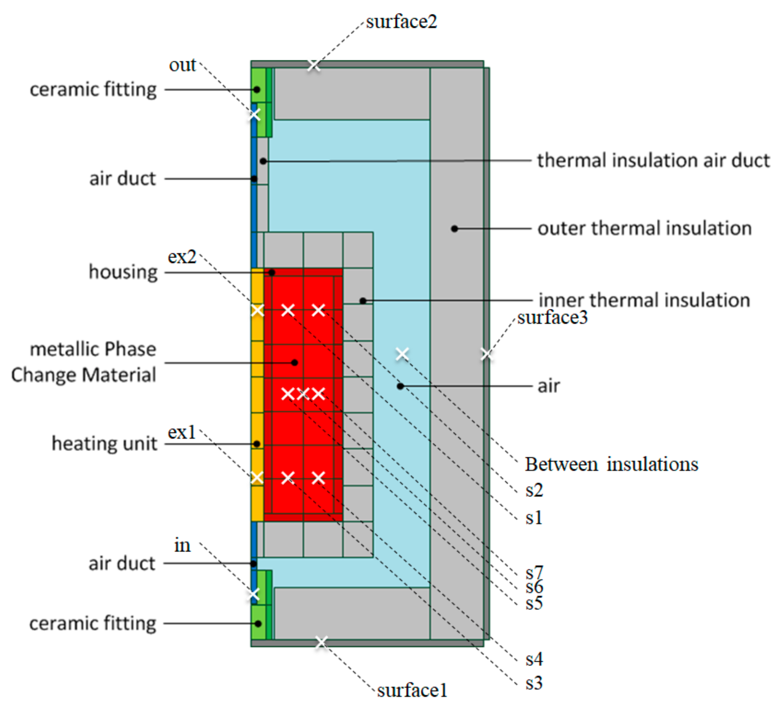
2.1. Simulated Specimen

The specimen simulated in the characterisation procedure potentially includes subcomponents like mPCM, container and heat transfer components. These heat transfer components are located in a central cylindrical tube, as proposed by Kraft and Klein Altstedde [4]. This study was performed with a sample mass of m_s = 5.688 kg. The chosen storage material was the eutectic alloy Al-12wt%Si, which was operated in a temperature range between 100 °C and 600 °C [4]. The storage material choice was made according to the storage concept proposed by Kraft and Klein Altstedde [4].

2.2. Methods

The aim of calorimetric characterisation of THS is to investigate the relevant thermophysical properties of the storage system. The properties are specific enthalpy of fusion h_fus, specific heat capacity c_p(ϑ) and melting temperature ϑ_fus. The specific state variables are gained by normalising to the sample mass m_s. The extrinsic values can be derived from the course of sample heat Q_S over sample temperature ϑ_S. Figure 1 shows a typical course of Q_S for a sample with first-order phase transition and its context with the mentioned relevant thermophysical properties. Here, only systems with a sharp melting temperature—not a melting temperature range—are considered (e.g., pure metals or eutectics). In general, it is possible to define the sample, not only as the storage material, but as the full system, including further system components like the housing. Hence, the boundaries of the sample can be defined depending on the matter of interest.

In Figure 1, the ideal course of Q_S is shown for a sample with a first-order phase transition. In Figure 2, it is qualitatively compared to a demonstrative “measured” Q_S-curve. Deviations from the ideal course result from a temperature gradient in the sample and test setup, which in turn means that the entire sample volume is not passing through the phase transition at the same time. This effect becomes more dominant the bigger the sample is. However, this effect is not expected to be very severe in this case, as metallic samples with high thermal conductivity minimise the thermal gradient [27].

The heat capacity C_p^{(ϑ1: ϑ2)} in a temperature range from ϑ₁ to ϑ₂ can directly be deduced from the slope of Q_s(ϑ):

$$C_{\mathrm{p}}^{{\vartheta }_1:{\vartheta }_2}=\frac{Q_{\mathrm{S}}\left({\vartheta }_2\right)-Q_{\mathrm{s}}\left({\vartheta }_1\right)}{{\vartheta }_2-{\vartheta }_1}$$

(1)

The specific heat capacity c_p can be derived from the relation to the sample mass m_s via c_p = C_p/m_s. As specific heat capacity is a temperature-dependent quantity, it is recommended to compare c_p values of different samples for similar temperature ranges. Enthalpy of fusion H_fus and melting temperature ϑ_fus are derived geometrically by the routine shown in Figure 3. This is a standardised routine described in DIN 51007.

Q_S is extrapolated linearly from the temperature ranges for C_p determination closest to the melting temperature (range for lower temperature: a; range for higher temperature: b) to ϑ_fus. This linear course of Q_S before the phase transition step is called the initial base line. ϑ_fus is defined as the intercept between the extrapolated initial base line and the inflection tangent of the step. The equation to determine H_fus is:

$$H_{\mathrm{fus}}=Q_{\mathrm{S}}\left({\vartheta }_1^{\mathrm{b}}\right)-Q_{\mathrm{S}}\left({\vartheta }_2^{\mathrm{a}}\right)-C_{\mathrm{p}}^{{\vartheta }_1^{\mathrm{b}}:{\vartheta }_2^{\mathrm{b}}}\cdot \left({\vartheta }_1^{\mathrm{b}}-{\vartheta }_{\mathrm{fus}}\right)-C_{\mathrm{p}}^{{\vartheta }_1^{\mathrm{a}}:{\vartheta }_2^{\mathrm{a}}}\cdot \left({\vartheta }_{\mathrm{fus}}-{\vartheta }_2^{\mathrm{a}}\right)$$

(2)

The specific enthalpy of fusion h_fus is determined via h_fus = H_fus/m_s.

In order to identify the calorimetric principles which cover all operational boundary conditions, a literature review mainly based on calorimeter classification by Sarge et al. [28] was performed. The characterisation procedure should be able to test the charging and discharging conditions of the storage. Heat output and input should be controllable in order to investigate the influence of the cooling and heating rates. Principles that are not suitable are listed below:

•

Isothermal calorimeters can only be operated at a defined temperature, thus it is not possible to test the whole operating temperature range of the specimen system.

•

Isoperibol calorimeters with uncontrolled heat exchange cannot fulfill the criterion of controllable heat input and output.

•

Isoperibol flow calorimeters are only suitable for fluid specimens.

•

Calorimeters with linear or nonlinear temperature changes of the surroundings are called scanning calorimeters. An essential component in the operation of scanning calorimeters is the time needed for heat exchange between the furnace and specimen. Depending on the heat path from the sample to the surroundings, the calorimeter signal can show a thermal lag [28,29]. Therefore, scanning calorimeters are not recommended for use with large sample sizes [30] and inhomogeneous samples, which is how the THS specimen system can be classified [31].

Suitable calorimetric principles are the isoperibol calorimeter with controlled heat exchange for both charging and discharging conditions and adiabatic calorimeters for charging conditions only. Three measurement procedures to realize these principles are proposed in this study. In order to keep the setup complexity as low as possible, procedures without a reference setup were used.

All proposed measuring procedures are based on solving a balancing equation of all heat amounts, resulting in the heat accumulation in sample Q_S at a certain sample temperature ϑ_S, referring to the chosen reference temperature ϑ_Ref. ϑ_S is logged over time t, making it possible to describe either Q_S(ϑ_S) or Q_S(t). Here, we chose to use the time-dependent values. The balancing equation, which can be used for every procedure, is:

Q_S(t) = Q_H(t) + Q_C(t) + Q_Loss(t) + Q_WF(t)

(3)

where Q_H is the heat input of the electrical heater, Q_C is the thermal energy in the components of the test bench, Q_Loss is the heat loss to the surroundings and Q_WF is the heat output by the working fluid. The difference between the procedures is in how the different contributions are determined. An overview is given in

Table 1. Overview of determination of each contribution to heat flow balance equation for different calorimetric measurement procedures.

Procedure	QH	QC	QLoss	QWF
Stepwise adiabatic	Measure PH	Measure (ϑC − ϑC,0)	Correlate to ϑSurface	Zero
Isoperibolic with loss correlation	Zero	Measure (ϑC − ϑC,0)	Correlate to ϑSurface	Measure (ϑout − ϑin) and $\dot{m}$
Isoperibolic with cooling correlation	Zero	Measure (ϑC − ϑC,0)	Correlate QCool to ϑex

P_H, power of electrical heater (W); ϑ_C, temperature of test bench components (°C); ϑ_C,0, Initial temperature of test bench components (°C); ϑ_Surface, temperature of test bench surface (°C); ϑ_Out, temperature of working fluid after passing sample (°C); ϑ_In, tempertuare of working fluid before passing sample (°C); Q_Cool, Q_Loss + Q_WF (J); ϑ_ex, temperature of heat exchanger in heat transfer zone of sample to working fluid (°C).

.

Q_C is always determined by measuring the difference of the components’ instantaneous temperature ϑ_C and initial temperature ϑ_C,0. With knowledge about the heat capacity of all test setup components C_C, the heat put into the components is described by:

$$Q_{\mathrm{C}}\left(t\right)=\left({\vartheta }_{\mathrm{C}}\left(t\right)-{\vartheta }_{\mathrm{C},0}\right)\cdot C_{\mathrm{C}}$$

(4)

The next sections describe the proposed measuring procedures in more detail.

2.2.1. Stepwise Adiabatic Procedure

In order to realise adiabatic conditions, the latent energy storage system is thermally isolated. Perfect adiabatic conditions, that is, where no heat is exchanged with the surroundings, cannot be achieved in reality. Thus, physical implementations are technically always isoperibolic, albeit with potentially very small heat loss [28,32].

Thermal energy is supplied to the thermally isolated sample via an electrical heater. If supply losses are neglected, heat input Q_H can be determined by electrical heating power P_H, which is supplied in the time interval between t_i and t_i+1:

$$Q_{\mathrm{H}}\left(t\right)=\underset{t_{\mathrm{i}}}{\overset{t_{\mathrm{i}+1}}{{\displaystyle \int }}}{P}_{\mathrm{H}}\mathrm{dt}$$

(5)

Heat loss Q_Loss cannot be directly measured but can be determined via calibration. To achieve this, the heater is power-controlled to hold the sample temperature constant for an equilibration time t_eq until a steady state is reached. Under steady state conditions, the total heating rate equals the heat flow into the setup components and the heat loss rate to the surroundings ${\dot{Q}}_{\mathrm{Loss}}$. The heat loss rate is then correlated to the surface temperature via a second-degree polynomial. The heat loss to the surroundings Q_Loss is finally received via integration over time. For this study, t_eq was chosen to be 45 min for each temperature range. The temperature step between 500 °C and 600 °C, t_eq, was chosen to be 60 min, as the phase change of the examined material Al-12wt%Si occurs in this temperature range.

2.2.2. Isoperibolic Procedure with Loss Correlation

In this procedure, the amount of thermal energy stored in sample Q_S is determined by measuring the heat balance of the working fluid which is cooling the sample. This procedure belongs to the class of isoperibol calorimeters with controlled heat exchange. Therefore, the sample is again thermally isolated, but this time, the working fluid is conducted through the central tube of the sample system. At first, the sample is heated to a maximum temperature by an electrical heater. Then, the heater is shut off and the flow of the working fluid is started. The heat transferred from the sample to the working fluid Q_WF is determined by measuring the temperature difference of the working fluid before passing sample ϑ_in and after passing sample ϑ_out. The mass flow rate $\dot{m}$ of the working fluid is set constant and the specific heat capacity of the working fluid c_p,WF is known. Q_WF can be determined via the following equation:

$$Q_{\mathrm{WF}}\left(t\right)=\dot{m}\cdot c_{\mathrm{p},\mathrm{WF}}\cdot \left({\vartheta }_{\mathrm{out}}\left(t\right)-{\vartheta }_{\mathrm{in}}\left(t\right)\right)$$

(6)

Q_Loss is determined via calibration and correlation during the heating phase, as described for the stepwise adiabatic procedure. Thus, calibration and measurement can be performed concurrently. For this procedure, t_eq = 30 min was chosen for calibration. The mass flow rate $\dot{m}$ was set to 50 kg/h.

2.2.3. Isoperibolic Procedure with Cooling Correlation

This procedure also belongs to the class of isoperibol calorimeters with controlled heat exchange. Again, the sample is isolated thermally and a working fluid is conducted through the centre of the sample. This time, the heat transferred to the working fluid Q_WF and the heat loss to the surroundings Q_Loss are not determined separately, but are combined in the expression Q_Cool = Q_WF + Q_Loss. Calibration is performed in order to correlate Q_Cool to the temperature of the heat exchanger ϑ_ex in the heat transfer zone of the sample to the working fluid. Therefore, the power of the electrical heater P_H is logged for different steady state temperature steps during heating. According to the other calibration methods, the following balance is true: ${\dot{Q}}_{\mathrm{H}}$ − ${\dot{Q}}_{\mathrm{C}}$ = ${\dot{Q}}_{\mathrm{Cool}}$. Cooling rate ${\dot{Q}}_{\mathrm{Cool}}$ is then correlated to ϑ_ex. It cannot be distinguished which amount of thermal energy is put out by the working fluid or by the loss to the surroundings. To keep the correlation as precise as possible, the working fluid’s mass flow $\dot{m}$ and the surrounding conditions need to be constant for both calibration and measurement. After the calibration and heating phase, the electrical heater is shut off, but the working fluid is kept flowing. Then, ϑ_ex(t) is logged over the cooling phase. For this procedure, t_eq = 30 min was chosen for calibration with active working fluid flow.

2.3. Experimental Setup

A test bench was designed to perform the proposed measurement procedures. In Figure 4, a schematic drawing of all parts relevant for the simulation is shown. The specimen for this study was a thermal energy storage consisting of an AISI 321 containment and the mPCM Al-12wt%Si. The container had the shape of a hollow cylinder with rounded edges and an empty mass of 3.3 kg, and was filled with m_s = 5.688 kg Al-12wt%Si cast into it. The heating unit was a hollow cylindrical copper piece with bore holes, into which 8 electric cartridge heaters were inserted within the central tube of the containment. Each cartridge heater had a maximum electrical power of 500 W. Within the centre of the heating unit, air could flow through the specimen for discharging. In order to enable high heat transfer, a heat transfer structure with fins was present in the hollow shape of the copper cylinder. The components of the air duct through the centre of the storage were thermally decoupled from the rest of the setup by ceramic fittings. The thermal energy storage component was surrounded by two layers of microporous thermal insulation to reduce thermal losses. PID controllers controlled the air mass flow and the heating power.

2.4. Simulation

For a transient simulative investigation of the measurement procedures, the Dymola simulation environment and the Modelica language were used to implement appropriate models. Sources for these models were the Modelica Standard Library v. 3.2.2 and Modelon Base Library v. 2.6 from Modelon AB, as well as in-house models, e.g., for the mPCM. As a solver, Esdirk45a (explicit singly diagonally implicit Runge-Kutta) [33] was used in this work.

For investigation of temperature gradients within components, several cells were assembled, where each cell consisted of a capacity and 4 heat conductors. This enabled heat conduction in 2 spatial dimensions. The discretisation level of each component was chosen in relation to the expected temperature gradient. The discretised simulation model is schematically displayed in Figure 5. Due to the rotational symmetry of most components, this approach results in a rotationally symmetric 2-dimensional model. For some test bench components, like the outer insulation layer, rotational symmetry is not true, which leads to a simplification of these parts. Due to their large lateral dimension compared to their small thickness, one-dimensional heat conduction through the outer insulation layer to the surroundings was also assumed.

The PID controllers for air mass flow control and heating power control were also included in the simulation model. In order to detect heat flows of interest authentically, virtual heat flow sensors were established in the simulation model. The copper cylinder with the dual function of heater and heat transfer body was geometrically simplified to a hollow cylinder. The geometry of the heat storage component itself was simplified to a cylindrical shape with a rectangular cross-section.

For the investigation of measurement procedures, different measured variables had to be logged, as outlined in Section 2.2. In the simulation model, only sensor positions that are accessible in the real setup were used. All sensors were assumed to operate ideally error-free. An overview of the measured variables and their corresponding sensor positions within the setup is shown in

Table 2. Temperature sensors used to measure relevant temperatures for procedure evaluation (for cylindrical components, logarithmic average was used). In italics are positions of sensors as marked in Figure 5.

Measure	Sensors
ϑs	Average of seven temperature sensors located in mPCM (s1–s7)
ϑsurface	Weighted average from three temperature sensors at the bottom, one side and top sheet (surface1–surface3)
ϑout	One temperature sensor (out)
ϑin	One temperature sensor (in)
ϑex	Average of two temperature sensors located at top and bottom of copper cylinder (ex1 and ex2)
ϑC	Components of test bench were divided into: Copper cylinder: ϑex Inner insulation: Average of ϑS and temperature sensor between insulations Outer insulation: Average of temperature sensor between insulations and ϑSurface Outer sheets: ϑSurface Containment: ϑS

. The indicated positions can also be found in Figure 5.

3. Results

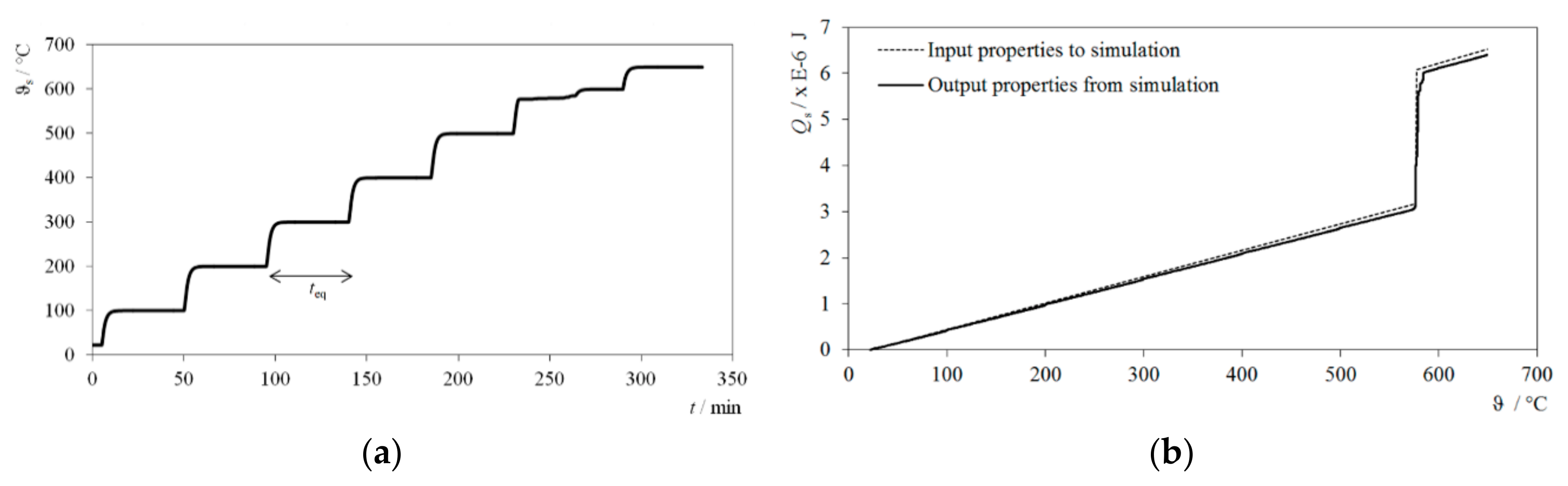
3.1. Stepwise Adiabatic Procedure

The course of sample temperature ϑ_S over time t for the stepwise adiabatic procedure is shown in Figure 6a. The temperature plateaus show the six equilibration steps where the heat loss to the surroundings was determined by measuring the heating power. The melting process of the storage material can be observed at an additional temperature plateau at 576.5 °C. The course of Q_S(ϑ) resulting from Equations (4) and (5) with temperature and power outputs of the simulation is shown in Figure 6b as well as the course of Q_S(ϑ) calculated from the simulation input values for c_p, ϑ_fus and h_fus. The slope of Q_S(ϑ), which corresponds to c_p, is observed to be lower in the simulation output than the input property. Thus, the overall amount of energy stored in the studied temperature range is underestimated.

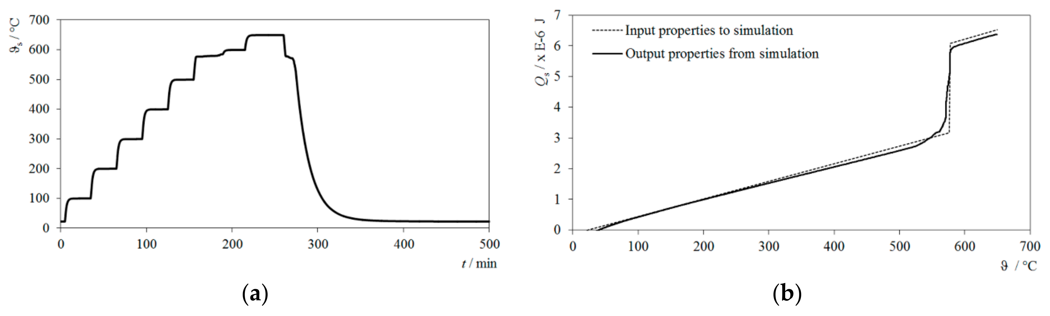
3.2. Isoperibolic Procedure with Loss Correlation

The course of sample temperature ϑ_S over time t for the isoperibolic procedure with loss correlation is shown in Figure 7a. The heating process for calibration and the cooling process for measurement can be seen. The course of Q_s resulting from simulation and the input course of Q_s are shown in Figure 7b. The simulated course of ϑ_s again shows the equilibration steps for heat loss determination and reveals the solidification process with an additional plateau at 576.5 °C. Upon further cooling, the temperature decreased more slowly and approximated room temperature asymptotically. The simulated course of Q_s revealed that c_p(ϑ) was not constant, although this was assumed for the input value. This interesting observation is elaborated further in the discussion. Again, the overall energy amount stored in the studied temperature range is underestimated. In contrast to the stepwise adiabatic procedure, this time Q_s resulted from a cooling half-cycle. This can be seen at the sharp edge at higher energy amounts, where solidification starts, and the diffuse transition to sensible cooling, as a solidification of the whole sample, takes some time.

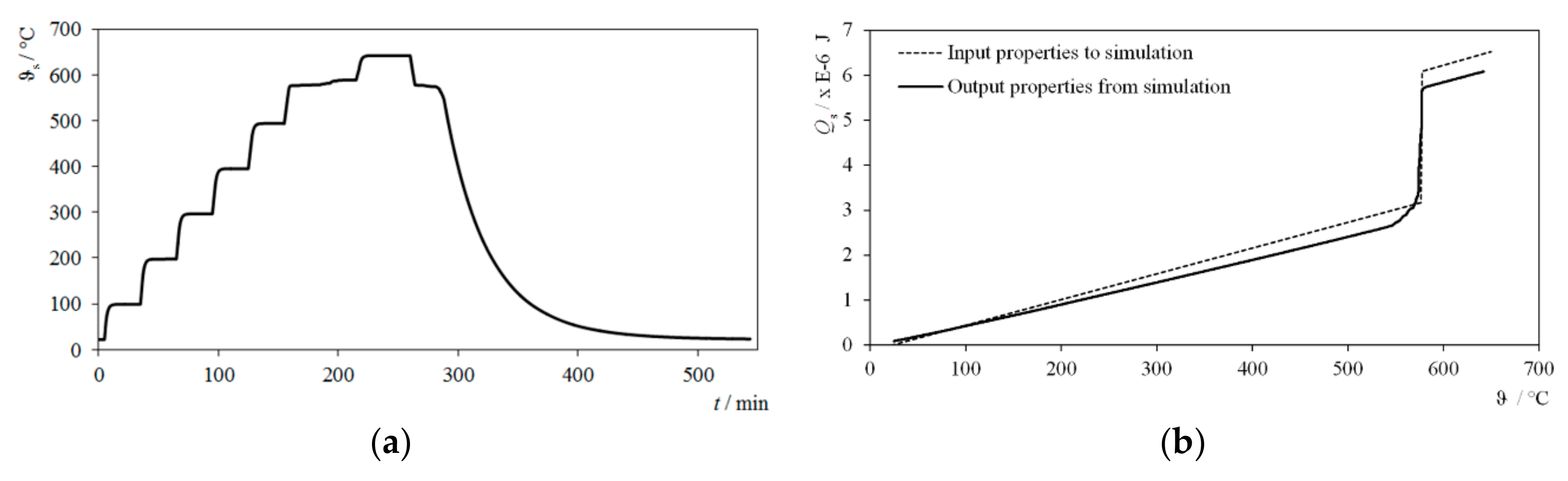
3.3. Isoperibolic Procedure with Cooling Correlation

The course of sample temperature ϑ_S over time t for the isoperibolic procedure with cooling correlation is shown in Figure 8a. The heating process for calibration and the cooling process for measurement can be seen. The course of Q_s resulting from simulation and the input course of Q_s are shown in Figure 8b. The simulation of ϑ_S shows a similar course as in the procedure with loss correlation. The simulated course of Q_S was nearly linear in the sensible range. However, the deviation of c_p in the solid range was visibly larger compared to the other procedures, and the energy stored in the studied temperature range was more greatly underestimated.

3.4. Deviation of Simulation Input Values

In order to evaluate the three proposed measuring procedures, simulated measured values were compared to the simulation input values for c_p(ϑ), ϑ_fus, h_fus and the overall stored energy in sample Q_S between 100 °C and 600 °C. The input values were determined via differential scanning calorimetry. An overview of the thermophysical properties generated by the different procedures in comparison to the input values is shown in Figure 9, with indication of the absolute deviation (primary ordinate) and relative deviation E (secondary ordinate).

The isoperibolic procedure with loss correlation shows the lowest error regarding the determination of c_p, but the largest deviation for h_fus. However, the isoperibolic procedure with cooling correlation shows contrasting behaviour. The assignment of stored energy to the sensible or the latent regime depends on the choice of extrapolation limits and the width of the now diffuse phase transition (compared with Figure 3). The stored heat in the whole temperature range Q_s^100:600 is a better indication for the accuracy of the procedure, as it is not as affected by these evaluation artefacts. Regarding this quantity, the stepwise adiabatic procedure has the lowest deviation from the simulation input value. However, this procedure is only suitable for analysing heating processes, not half-cycles with active cooling.

4. Discussion

In the simulation, all sensors were assumed to operate ideally error-free. The results of this study therefore only reflect the deviations resulting from the courses and setups of the different procedures themselves and numerical inaccuracy. In a real test setup, additional uncertainties of measurement from the sensors have to be considered.

Phase change characteristics: The melting step resulting from simulation is not as sharp as in the input. The reason could be a temperature gradient in the storage material upon melting. For the procedures where the cooling half-cycle is evaluated, the liquidus temperature can be determined more precisely and the solidus temperature is very diffuse. For the stepwise adiabatic procedure, only the heating half-cycle is evaluated, therefore the solidus temperature can be observed well but the liquidus temperature is diffuse.

Correlation temperature: The correlation temperature used for calibration has a significant systematic influence on the output. Thermal inertia in the system can lead to an incorrect estimation of heat loss if an unsuitable correlation temperature is chosen. Depending on the position of the correlation temperature, large thermal inertia can lead to the situation that no thermal equilibrium between correlation and sample temperature is reached after equilibration time during heating. Furthermore, a completely different thermal gradient can arise during cooling, so that the correlation function is no longer transferable from the heating to the cooling half-cycle.

Equilibration time: A further significant influence on the quality of calibration is the time chosen to reach steady state conditions during calibration. All procedures underestimated c_p, which could result from a temperature gradient in the sample setup, meaning that steady state was not reached in the chosen time t_eq. Thus, Q_Loss was overestimated and c_p underestimated. The deviation of c_p for t_eq = 45 min was smaller than for a tested alternative with t_eq = 30 min, as the state between the temperature steps was closer to steady state conditions. This suggests that increasing t_eq leads to increased accuracy in the determination of c_p and especially heat losses. Increasing the time step allows large thermal inertias to equilibrate, but this increases experiment time. An optimum between correlation temperature and equilibration time should be determined when commissioning physical experiments. In the simulation, thermal inertia only results from bulk thermal resistance, whereas in the experiment, thermal contact resistance also needs to be considered. Thermal contacts are strongly geometry-dependent and are affected by thermal expansion and the properties of layers or coatings at interfaces. For storage systems with poor thermal contact, the accuracy of the procedures can be reduced if the equilibration time is not increased.

Heat loss: Another important aspect that influences the accuracy of the result is the proportion of heat lost in the total energy balance Equation (3). For the stepwise adiabatic procedure, deviations between simulation input and output values increased with increasing temperature as the ratio between lost thermal energy Q_Loss and stored thermal energy Q_S increased. For the isoperibolic procedure with loss correlation, the biggest deviation between simulated and input c_p occurred at low temperatures, where the cooling rate is slowest. The slower the cooling, the faster Q_WF decreases compared to Q_Loss and the larger the proportion of Q_Loss in the total balance. The accuracy of this procedure might be increased by increasing the portion of Q_WF in the total balance with an increased mass flow rate of coolant. Similar behaviour was observed for the isoperibolic procedure with cooling correlation. However, in this procedure, the working fluid mass flow cannot be increased without limit, as the thermal output is not allowed to be larger than the thermal input realisable by the installed electrical heaters.

Numerical inaccuracy: Potential numerical inaccuracy can depend on the chosen time increment used for simulation and the residual error of the solver. These did not have considerable influence.

5. Conclusions

Three measuring procedures for the thermophysical characterisation of THS utilising mPCM at the system scale were derived and described. A test setup was designed and the procedures were examined through simulation. All sensors were assumed to operate ideally error-free so that deviations resulted only from the course of each procedure and potentially numerical inaccuracy. The most suitable procedure to determine the overall stored heat in the specimen system was the stepwise adiabatic procedure. However, this procedure is limited to heating processes and cannot be used to test half-cycles with active cooling. The accuracy of isoperibolic procedures involving either loss or cooling correlation depends on several parameters, including the extrapolation limits, the correlation temperature, the equilibration time, the mass flow of the working fluid and the thermal contact between thermal subsystems. The procedures could be optimised by adjusting these parameters through a sensitivity analysis. For a final evaluation of the proposed procedures, it is necessary to additionally assess errors that arise from the sensors and devices. The procedures outlined in this work provide a first step for commissioning an experimental apparatus. This device may be used to validate the absolute outputs of the simulation and check the reproducibility of the proposed procedures.

References

1. Neubauer, J.; Wood, E. Thru-life impacts of driver aggression, climate, cabin thermal management, and battery thermal management on battery electric vehicle utility. J. Power Sources 2014, 259, 262–275. [Google Scholar] [CrossRef]
2. Kambly, K.; Bradley, T.H. Geographical and temporal differences in electric vehicle range due to cabin conditioning energy consumption. J. Power Sources 2015, 275, 468–475. [Google Scholar] [CrossRef]
3. Yuksel, T.; Michalek, J.J. Effects of regional temperature on electric vehicle efficiency, range, and emissions in the United States. Environ. Sci. Technol. 2015, 49, 3974–3980. [Google Scholar] [CrossRef]
4. Kraft, W.; Altstedde, M.K. Use of metallic Phase Change Materials (mPCM) for heat storage in Electric- and Hybrid Vehicles. In Proceedings of the Tagungsband 6th Hybrid and Electric Vehicles Conference (HEVC 2016), London, UK, 2–3 November 2016; pp. 1–6. [Google Scholar]
5. Kraft, W.; Jilg, V.; Klein Altstedde, M.; Lanz, T.; Vetter, P.; Schwarz, D. Thermal High Performance Storages for Use in Vehicle Applications; Springer: Cham, Switzerland, 2018. [Google Scholar]
6. Gasia, J.; Miró, L.; Cabeza, L.F. Materials and system requirements of high temperature thermal energy storage systems: A review. Part 2: Thermal conductivity enhancement techniques. Renew. Sustain. Energy Rev. 2016, 60, 1584–1601. [Google Scholar] [CrossRef] [Green Version]
7. Ibrahim, N.I.; Al-Sulaiman, F.A.; Rahman, S.; Yilbas, B.S.; Sahin, A.Z. Heat transfer enhancement of phase change materials for thermal energy storage applications: A critical review. Renew. Sustain. Energy Rev. 2017, 74, 26–50. [Google Scholar] [CrossRef]
8. Birchenall, C.E.; Riechman, A.F. Heat Storage in Eutectic Alloys. Metall. Trans. A 1980, 11, 1415–1420. [Google Scholar] [CrossRef]
9. Khare, S.; Dell’Amico, M.; Knight, C.; McGarry, S. Selection of materials for high temperature latent heat energy storage. Sol. Energy Mater. Sol. Cells 2012, 107, 20–27. [Google Scholar] [CrossRef]
10. Shamberger, P.J.; Bruno, N.M. Review of metallic phase change materials for high heat flux transient thermal management applications. Appl. Energy 2020, 258, 113955. [Google Scholar] [CrossRef]
11. Kraft, W.; Stahl, V.; Vetter, P. Thermal Storage Using Metallic Phase Change Materials for Bus Heating—State of the Art of Electric Buses and Requirements for the Storage System. Energies 2020, 13, 3023. [Google Scholar] [CrossRef]
12. Yinping, Z.; Yi, J. A simple method, the -history method, of determining the heat of fusion, specific heat and thermal conductivity of phase-change materials. Meas. Sci. Technol. 1999, 10, 201–205. [Google Scholar] [CrossRef]
13. Solé, A.; Miró, L.; Barreneche, C.; Martorell, I.; Cabeza, L.F. Review of the T -history method to determine thermophysical properties of phase change materials (PCM). Renew. Sustain. Energy Rev. 2013, 26, 425–436. [Google Scholar] [CrossRef]
14. Cabeza, L.F.; Barreneche, C.; Martorell, I.; Miró, L.; Sari-Bey, S.; Fois, M.; Paksoy, H.O.; Sahan, N.; Weber, R.; Constantinescu, M.; et al. Unconventional experimental technologies available for phase change materials (PCM) characterization. Part 1. Thermophysical properties. Renew. Sustain. Energy Rev. 2015, 43, 1399–1414. [Google Scholar] [CrossRef] [Green Version]
15. Navrotsky, A. New Developments in the Calorimetry of High-Temperature Materials. Engineering 2019, 5, 366–371. [Google Scholar] [CrossRef]
16. Binder, S.; Haussener, S. Design guidelines for Al-12%Si latent heat storage encapsulations to optimize performance and mitigate degradation. Appl. Surf. Sci. 2020, 505, 143684. [Google Scholar] [CrossRef]
17. Günther, E.; Hiebler, S.; Mehling, H. Determination of the Heat Storage Capacity of PCM and PCM-Objects as a Function of Temperature. In Proceedings of the ECOSTOCK 10th International Conference on Thermal Energy Storage, Stockton, NJ, USA, 31 May–2 June 2006. [Google Scholar]
18. Rathgeber, C.; Schmit, H.; Miró, L.; Cabeza, L.F.; Gutierrez, A.; Ushak, S.N.; Hiebler, S. Enthalpy-temperature plots to compare calorimetric measurements of phase change materials at different sample scales. J. Energy Storage 2018, 15, 32–38. [Google Scholar] [CrossRef] [Green Version]
19. Xu, T.; Gunasekara, S.N.; Chiu, J.N.; Palm, B.; Sawalha, S. Thermal behavior of a sodium acetate trihydrate-based PCM: T-history and full-scale tests. Appl. Energy 2020, 261, 114432. [Google Scholar] [CrossRef]
20. Klimeš, L.; Charvát, P.; Mastani Joybari, M.; Zálešák, M.; Haghighat, F.; Panchabikesan, K.; El Mankibi, M.; Yuan, Y. Computer modelling and experimental investigation of phase change hysteresis of PCMs: The state-of-the-art review. Appl. Energy 2020, 263, 114572. [Google Scholar] [CrossRef]
21. Zauner, C.; Hengstberger, F.; Mörzinger, B.; Hofmann, R.; Walter, H. Experimental characterization and simulation of a hybrid sensible-latent heat storage. Appl. Energy 2017, 189, 506–519. [Google Scholar] [CrossRef]
22. Jansone, D.; Dzikevics, M.; Veidenbergs, I. Determination of thermophysical properties of phase change materials using T-History method. Energy Procedia 2018, 147, 488–494. [Google Scholar] [CrossRef]
23. Waser, R.; Ghani, F.; Maranda, S.; O’Donovan, T.S.; Schuetz, P.; Zaglio, M.; Worlitschek, J. Fast and experimentally validated model of a latent thermal energy storage device for system level simulations. Appl. Energy 2018, 231, 116–126. [Google Scholar] [CrossRef]
24. Pirasaci, T.; Wickramaratne, C.; Moloney, F.; Goswami, D.Y.; Stefanakos, E. Influence of design on performance of a latent heat storage system at high temperatures. Appl. Energy 2018, 224, 220–229. [Google Scholar] [CrossRef]
25. Rea, J.E.; Oshman, C.J.; Singh, A.; Alleman, J.; Parilla, P.A.; Hardin, C.L.; Olsen, M.L.; Siegel, N.P.; Ginley, D.S.; Toberer, E.S. Experimental demonstration of a dispatchable latent heat storage system with aluminum-silicon as a phase change material. Appl. Energy 2018, 230, 1218–1229. [Google Scholar] [CrossRef]
26. Rea, J.E.; Oshman, C.J.; Singh, A.; Alleman, J.; Buchholz, G.; Parilla, P.A.; Adamczyk, J.M.; Fujishin, H.-N.; Ortiz, B.R.; Braden, T.; et al. Prototype latent heat storage system with aluminum-silicon as a phase change material and a Stirling engine for electricity generation. Energy Convers. Manag. 2019, 199, 111992. [Google Scholar] [CrossRef]
27. Blanco-Rodríguez, P.; Rodríguez-Aseguinolaza, J.; Gil, A.; Risueño, E.; D’Aguanno, B.; Loroño, I.; Martín, L. Experiments on a Lab Scale TES Unit using Eutectic Metal Alloy as PCM. Energy Procedia 2015, 69, 769–778. [Google Scholar] [CrossRef] [Green Version]
28. Sarge, S.M.; Höhne, G.W.H.; Hemminger, W. Calorimetry. Fundamentals, Instrumentation and Applications, 2nd ed.; Wiley-VCH Verlag: Weinheim, Germany, 2014; ISBN 978-3-527-32761-4. [Google Scholar]
29. Mathis, D.; Blanchet, P.; Landry, V.; Lagière, P. Thermal characterization of bio-based phase changing materials in decorative wood-based panels for thermal energy storage. Green Energy Environ. 2019, 4, 56–65. [Google Scholar] [CrossRef]
30. Quick, C.R.; Schawe, J.E.K.; Uggowitzer, P.J.; Pogatscher, S. Measurement of specific heat capacity via fast scanning calorimetry—Accuracy and loss corrections. Thermochim. Acta 2019, 677, 12–20. [Google Scholar] [CrossRef]
31. Shukla, N.; Kosny, J. DHFMA Method for Dynamic Thermal Property Measurement of PCM-integrated Building Materials. Curr. Sustain. Renew. Energy Rep. 2015, 2, 41–46. [Google Scholar] [CrossRef] [Green Version]
32. Bessergenev, V.G.; Kovalevskaya, Y.A.; Paukov, I.E.; Shkredov, Y.A. Heat capacity measurements under continuous heating and cooling using vacuum adiabatic calorimetry. Thermochim. Acta 1989, 139, 245–256. [Google Scholar] [CrossRef]
33. Kværnø, A. Singly Diagonally Implicit Runge–Kutta Methods with an Explicit First Stage. BIT Numer. Math. 2004, 44, 489–502. [Google Scholar] [CrossRef]
Figure 1. Context of thermophysical properties enthalpy of fusion Hfus, heat capacity Cp(ϑ) and melting temperature ϑfus with course of sample heat QS over sample temperature ϑS referred to reference temperature ϑRef.
Energies 14 02241 g001
Figure 2. Ideal (solid) and measured (broken) curve of QS over ϑS of sample with first-order phase transition.
Energies 14 02241 g002
Figure 3. Schematic routine to derive enthalpy of fusion Hfus and melting temperature ϑfus geometrically from QS curve.
Energies 14 02241 g003
Figure 4. Schematic drawing of test bench. Component labelled “thermal energy storage” is the specimen for this study and consists of AISI 321 containment filled with mPCM Al-12wt%Si.
Energies 14 02241 g004
Figure 5. Discretisation of relevant components within simulation model and sensor positions.
Energies 14 02241 g005
Figure 6. Results of stepwise adiabatic procedure. (a) Course of simulated sample temperature over time with teq = 45 min. (b) Course of QS curve resulting from simulation (solid) compared to curve resulting from simulation input values (broken).
Energies 14 02241 g006
Figure 7. Results of isoperibolic procedure with loss correlation. (a) Course of simulated sample temperature over time with teq = 30 min and m ˙ = 50 kg/h. (b) Course of QS curve resulting from simulation (solid) compared to curve resulting from simulation input values (broken).
Energies 14 02241 g007
Figure 8. Results of isoperibolic procedure with cooling correlation. (a) Course of simulated sample temperature over time with teq = 30 min and m ˙ = 20 kg/h. (b) Course of QS curve resulting from simulation (solid) compared to curve resulting from simulation input values (broken).
Energies 14 02241 g008
Figure 9. Absolute values of measuring procedures referring to simulation input values (maximum of primary ordinate) and relative deviation E (secondary ordinate). Procedure 1 = stepwise adiabatic procedure; 2 = isoperibolic procedure with loss correlation; 3 = isoperibolic procedure with cooling correlation. (a) Specific heat capacity between 50 °C and 500 °C; (b) specific heat capacity between 600 °C and 650 °C; (c) temperature of fusion; (d) specific heat of fusion; (e) heat stored in specimen between 100 °C and 600 °C.
Energies 14 02241 g009