“Green Energy” and the Standard of Living of the EU Residents

Abstract

The author intended to present the relationship between the standard of living of EU citizens and the level of the development of renewable energy. It is particularly important in the context of the implementation of the sustainable development idea, by ensuring a high standard of living for both current and future generations, with rational use of available natural resources. The first, theoretical part of the article presents the problem related to the impact of renewable energy on the standard of living in a synthetic way. The second part involves empirical research conducted in all countries of the EU. To evaluate the level of renewable energy development and the standard of living, the author constructed original measures based on the TOPSIS method. Variables were selected on the basis of substantive, statistical and formal criteria (primarily the completeness and availability of data in 2019). Within the framework of the conducted study, the author obtained, among other things, a relatively high value of Spearman’s rank correlation coefficient between the constructed synthetic measures (0.47). Canonical analysis was used to identify the relationship between them. Numerous indicators, including canonical correlations, complete redundancy and extracted variances, were determined with the use of canonical analysis. Seven statistically significant canonical variables were identified. The value of the greatest and most statistically significant canonical correlation exceeded 0.94, and for the last statistically significant canonical variable, the value reached over 0.31. Statistical data were primarily obtained from the publicly available EUROSTAT database.

1. Introduction

It is hard to disagree that energy, regardless of its form, constitutes the basis of any economic activity. Availability of energy is currently the basis of human existence and society will become more and more dependent on energy sources, mostly since all kinds of everyday devices are powered with electricity. The development of electricity (the increase in uninterrupted energy supply) has played a special role in health care, decreasing infant mortality, development of agricultural production and industry, thus affecting the standard of living of the population. Electric energy will remain an important determinant of an adequate standard of living and the importance of energy security in each country (broadly understood as the ability to satisfy the demand for energy in terms of quantity and quality, at the lowest price possible and maintaining environmental protection) will grow. Due to these demands, new sources of energy are needed. The demand for energy increasing along with civilizational progress [1], as well as the simultaneous depletion of discovered and accessible conventional energy sources (mainly fossil fuels) and progressive degradation of the environment, makes renewable energy sources (the so-called “green energy”) the desired direction for energy generation. As a result, renewable energy sources (the so-called “green energy”) has become desired methods of energy production. Various solutions, adapted to regional and local conditions, are adopted for this purpose. Energy is obtained with the use of the wind, the sun, tides and ocean currents, river drops, or energy obtained from biomass (most often hay from crop cultivation and firewood). Landfill biogas and biogas obtained from sewage disposal processes or decomposition of components of plant or animal remains are also listed among such sources. The increase in the importance of such energy sources stems from, among other things, their positive impact on the environment or increasing of energy security (apart from the effective way of storing the produced energy). It is particularly important in the context of the implementation of the sustainable development idea, by ensuring a high standard of living for both current and future generations, with rational use of available natural resources. For this reason, increasing the share of energy obtained from renewable sources in energy balances of different countries constitutes an important aspect of the adopted sustainable development strategy. At this point, it must also be noted that a sort of coexistence of renewable energy sources and modern ways of utilising conventional energy sources (e.g., lignite) sometimes occurs as well. An example is Germany, one of the leaders in the European Union [1] (and in the world in general) in terms of lignite mining; at the same time, in the first quarter of 2019, the share of renewable energy in the amount of electricity supplied in Germany surpassed the share of electricity generated there using fossil fuels. [2].

Although the Europe 2020 Strategy is about to expire, this approach is in line with the “TOWARDS A SUSTAINABLE EUROPE BY 2030” document, which envisions a European Union-level transition to a low-carbon, climate-neutral, resource-efficient and biodiverse economy [3]. In turn, according to the European Green Deal strategic programme established by the European Commission, the goal is to make Europe a climate-neutral continent by 2050. The most important initiatives included in the programme are achieving global CO₂ emissions neutrality, incorporating a wide range of renewable energy sources into the energy system, establishing a circular economy and achieving zero emissions of pollutants [4].

In the subject literature, the impact of renewable energy on the standard of living was analysed in the context of energy poverty (by such scholars as C.W. Njiru and S.C. Letem [5], E.M. Getie [6], or M.A. Hussein and W.L. Filho [7].

In the literature, the problem of the impact of renewable energy on the standard of living has been analysed in the context of energy poverty. Less frequently renewable energy is strictly treated as a livelihood enabler.

This article aims to determine the correlation between the level of renewable energy development and the standard of living of EU citizens. An additional goal assumed by the author was to popularize the relatively rarely used canonical analysis. The aim, however, was not to scrupulously explain this calculation method in detail, but rather demonstrate its usefulness. To create a measurement tool for the analysed phenomena, the author used a multi-dimensional comparative analysis, which was a set of methods of the construction of synthetic measurements and linear ordering of objects described by a large number of variables (including the TOPSIS method). A correlation analysis was conducted to determine the direction and the strength of the correlation between the constructed, original synthetic measures of the standard of living and the level of “green energy” development. On the other hand, the author used canonical analysis, one of the advanced methods of multidimensional statistical analysis, to identify multidimensional correlations between the standard of living and the level of renewable energy development. The study involved 27 member states of the EU. Statistical data obtained from international statistical institutions, mainly EUROSTAT [8], were used in the paper. The data concerned the year 2019.

2. The Standard of Living and Renewable Energy—The Theoretical Aspect

The notion of the standard of living is commonly applied in everyday life while its meaning varies, which results primarily from the fact that it constitutes the subject of research in many scientific fields (including sociology, philosophy, economics, physiology, or psychology). On the one hand, there is a broad interdisciplinary research perspective—both problem-related and methodological—while on the other hand, there is a problem of operationalisation of this research category. What is missing in the numerous and constantly evolving literature on the subject is one commonly accepted definition.

In 1954, the UN expert committee defined the standard of living of the inhabitants as the entirety of their actual living conditions, as well as the level of material and cultural satisfaction of needs through numerous goods and paid services, as well as those derived from the social funds (quoted after [9]). This interpretation has become the basis for many other definitions, formulated in the future. A. Luszniewicz (1982) defined the standard of living as the degree to which material and cultural needs of households are met (i.e., its security) through the streams of paid goods and services and funds for collective consumption [10]. U. Grzega considered the standard of living to be “the degree of satisfaction of human needs, resulting from the consumption of material goods and services, as well as the use of the values of the natural and social environment” [11]. According to One Global Economy, the standard of living is, first and foremost, defined by three categories [12]: income (changes in annual income, savings, employment and career, entrepreneurship); education (finishing high school, university admission); health (availability of the health care system, disease management programmes, preventive medicine (including prenatal care, sanitation services, vaccinations).

The category if the standard of living is largely based on the theory of needs (see:

Table 1. Categories of human needs.

Max-Neef [10]	1. Subsistence; 2. Protection; 3. Affection, 4. Understanding; 5. Participation; 6. Idleness; 7. Creation; 8. Identity; 9. Freedom.
Słaby [6]	1. Biological condition (food, housing, health, natural environment, leisure); 2 Professional status (having a job, working hours, wages); 3. Material status (savings, prices, durable goods); 4. Educational status (education of children and youth, education of adults, culture and art); 5. Social status (social security, income egalitarianism, social pathology, family and social bonds, politics).
Murray, Pauw, Holm [11]	1. Subsistence; 2. intactness, arrangement, intake, waste, movement, temperature, receptivity); 2. Protection (e.g., maintain physical subsistence);3. Affection (e.g., pleasure, trust, loyalty, respect); 4. Participation (receiving, giving); 5. Understanding (perception, cognition, emotion, reflex); 6. Creation (transform matter, transform symbols, procreate). 7. Idleness (catharsis, revitalization); 8. Identity (e.g., physical disposition and appearance, personality); 9. Freedom (choice, value); 10. Transcendence (affirmation of life, overcome meaninglessness).
Ding, Jiang, Riloff [12]	1. Physiological Needs; 2. Physical Health and Safety Needs; 3. Leisure and Aesthetic Needs; 4. Social, Self-Worth, and Self-Esteem Needs; 5. Finances, Possessions, and Job Needs; 6. Cognition and Education Needs; 7. Freedom of Movement and Accessibility Needs.

Source: own elaboration based on [13,17,18,19].

). If human needs are satisfied to a large extent, it means that the standard of living is high. A need is defined as a perceived state of absence of something, while social needs are needs whose fulfilment requires the existence and action of various social institutions for the intended purposes. A characteristic feature of needs is their variability over time, which is less related to basic needs (e.g., food, shelter) and more to the higher (luxurious) ones [13]. According to A. Chabior et al., a need is a state of a deficiency, absence, imbalance in the qualities of the organism or environment that are important to a person. Therefore, a need means a lack of something that motives one to initiate action aimed at compensating for such lack and restoring the disturbed optimum in life [14]. According to K.W. Frieske and P. Poławski needs are conditions that must be met to make people able to cooperate, take autonomous decisions and in general participate in collective life [15]. In T. Tomaszewski’s approach, the most detailed needs mentioned in the literature can be classified into three categories: biological (or elementary) needs, social needs and cultural needs. Social or elementary needs are understood as needs related to the structure of the human organism, the satisfying of which is necessary to keep a given organism or species alive (the need for food, water, oxygen). In turn, based on the fact that humans are in a certain sense dependent on others, we can distinguish social needs (such as the need to be accepted by others, the need to be loved or recognized). The third group of needs constitutes an expression of human dependency on the creations of human culture and the operation of social institutions. Such needs can be called cultural needs, which include products of material culture (accommodation, radio, fridge, car) and creations of spiritual culture (books, the cinema and the theatre, social conversation) [16].

T. Słaby observes that in terms of economy the need to have or feel for any purpose constitutes the basis for the production and exchange of goods. The need for goods and services constitutes the basic component of rational environmental management towards sustainable development [20].

As a multidimensional phenomenon, the diversity of the standard of living is conditioned by several factors, which generally may be divided into external and internal. External factors influence the variability of the said standards in time, while internal factors-in space. Internal factors are directly or indirectly influenced by the inhabitants of a given region. This group of factors includes, among others, the manner of managing the local self-government unit, which is reflected in the organisation of life (spatial plans and their implementation, the location of jobs, housing construction, provision of social, educational, health and other services) and the level of economic development. External factors include the dynamics of population development and its structure, as well as equipment with the technical infrastructure [21]. According to J. Piasny, in socio-economic terms, the standard of living includes all circumstances characterizing material and cultural as well as social conditions of the life of society. According to the author, the determinants include work conditions (e.g., whether it was easy to obtain it, its difficulty, the length of the working week), wage or income level, consumption, housing situation, the possessed durable consumer goods, the level of health and social care, the condition of education and culture, the provision of water to households, gas, electricity, sewage systems etc. [22].

Disparities in the level of life and social inequalities (like the use of renewable energy sources) have recently become a persistent focus of economic analyses. A. Zeliaś [23] explains the growing interest of researchers in the economic category that is the standard of living with the transition from the stage of fascination with the pace of technical and economic progress into the stage of reflection on the benefits and dangers of the civilizational progress. The adverse phenomena that economic brings include [24,25]: accelerated degradation of the natural environment, threatening the lives of humans and animals; a significant increase in morbidity and premature deaths due to certain diseases, mainly the so-called “civilization diseases” (such as cardiovascular diseases, cancer); an increase in various social pathologies (such as frustration, crime, alcoholism); a rapid increase in the number of traffic accidents and accidents at work; disorientation in the value system, destruction of old systems without the creation of new ones instead; an increase in social disparities in various social cross-sections and so on; excessive consumption of products and goods, resulting in environmental pollution; inability to produce substitutes for non-renewable resources without increasing ecological risk for the environment and humans.

In recent decades, amidst the transformation of many EU economies, the standard of living was determined by many factors as well as socio-economic and political processes. Nowadays, environmental issues, including the use of renewable energy sources, are becoming particularly important.

The contemporary economic system is characterized by cost externalization and “non-payment of bills” as well as the “grow first and clean up later” strategy. As a result of this phenomenon, there is an imbalance in the economic system, which is reflected in environmental pollution of water, air and land. Increasing environmental pollution has an impact on the standard of living and production capacity—production costs are growing because technological processes require the use of clean water and clean air. In the long term, it may lead to irreversible changes in the natural environment [26]. As it has already been mentioned, ensuring a high standard of living to both current and future generations with rational use of the available natural resources constitutes a basic prerequisite for sustainable development. Such an approach dominates international economic relations, and in recent decades we have been observing a concentration of actions oriented towards the transformation of socio-economic systems into the so-called green economy.

The concept of a “green economy” is relatively new. The term itself first appeared in 1989 in the report entitled Blueprint for a Green Economy, prepared for the government of Great Britain (to support the introduction of the sustainable development idea) by D. Pearce, A. Markandya and E.B. Barbier [27]. From the perspective of these considerations, it is worth quoting the definition of “green economy” adopted by UNEP, which provides that it is an economy that improves welfare and social equality (justice) while reducing environmental risk and the use of natural resources [28]. It can be assumed that an important role in the initiation thereof was played by the United Nations Environmental Protection Programme of 2008, which called for the conclusion of an agreement, the so-called Global Green New Deal, within the framework of which opportunities and chances to recover from the global economic crisis through the development of “green” economy sectors were indicated. The Global Green New Deal. Policy Brief report, published in 2009, recommended investing in environmentally important areas with the greatest potential for transformation, headed towards “green economy”, such as, among other things: renewable energy, clean technologies, energy-efficient construction, recycling and waste management, sustainable use of land, green coal mining techniques (including the underground coal gasification process) [29]. Energetic self-sufficiency, defined by the ratio of the amount of energy obtained to the amount of energy used in a given country/region, became one of the most important indicators characterizing sustainable development [30]. The green economy thus becomes a path to achieve sustainable development.

The concept of sustainable development is supposed to contribute to solving the main challenges of contemporary economies, which comprise fears related to climate changes and excessive air pollution, but also depletion of natural resources and energy security. In the face of these challenges, the development of renewable energy seems to be an important element in the implementation of the new energy policy. Two main areas can by confirmed by the effects of implementing sustainable development:

• production and consumption, where it is expected that natural resources will be used in a rational way and energy will be used effectively, waste and poverty will be reduced and economic competitiveness will be strengthened.
• energy use and production, where it is expected that air quality will be improved, the energy intensity of production will be reduced, energy efficiency will be improved and that energy security and general access to clean energy will be increased. The area assumes that it is critically important to increase the use of renewable energy sources and slowly become less dependent on traditional energy sources (including oil and natural gas) [31].

The processes of transitioning to a low-carbon fossil-fuel-free economy to a certain extent stem from the obligations imposed on governments and national economies by international organizations, mainly within the framework of the United Nations Framework Convention on Climate Change (UNFCCC or FCCC) and the Kyoto Protocol, and partially result from the emergence of new technologies and innovations that are climate-friendly and provide a competitive advantage [32]. Although the guidelines stemming from the concept of the green economy should not be ignored by any country, the condition and implementation thereof in most of them is still not satisfactory. The basic problem in many countries is not the amount of energy produced and used, but the fact that the source thereof are fossil fuels. It is estimated that the total technical potential of renewable energy can be 100 times higher than the current global demand for energy [33].

Nowadays, the energy needs of consumers are impacted by a wide variety of factors, including the level of development of a society to which a consumer belongs, economic and cultural traditions; geographical location; mobility and development aspirations and so on [34].

Until 2050, the technological revolution will take place not only with a share of an increase in energy efficiency and renewable energy sources but also with a growing role of energy prosumers in the economy [35]. Therefore, the involvement of the main stakeholders-citizens of individual countries and regions, who must participate in the creation of their (as well as local/regional) energy security—is necessary to make the energy revolution possible. Already in 1947, M. McLuhan and B. Nevitt [36] formulated a thesis that with the development of new electrical technologies, the consumer will be increasingly often becoming the producer. Businesses (including households) using new technological solutions for the production of electricity (and/or heat energy) that satisfies their needs are referred to as prosumers in the energy market. A prosumer is a participant in the prosumption process, in other words—both a user and a consumer, producing a product to consume it on its own. A prosumer is an active consumer-customer, who not only buys electricity (and/or heat energy) from traditional suppliers but also engages in active purchase and sale relations with them. It produces energy with the use of distributed power generation equipment (DPGE) and sales the surplus. It also sells system services, such as demand reduction. It is equipped with storage DPGE technologies which provide it with back up power, especially electricity, in the case of grid failures [37]. Pro-consumer energy represents the lowest level of distributed energy. It includes such microgeneration installations as solar collectors, photovoltaic microsystems, biomass boilers, micro wind turbines, biogas-powered cogeneration microsystems, heat pumps. The most important prosumer groups include households, small and medium-sized farms as well as small and medium-sized enterprises (located mainly in rural and suburban areas).

The development of prosumer energy has many benefits for prosumers (it impacts the standard of living in the case of households), national economies and the environment. The benefits are as follows [38]: a prosumer lives in a household that generates profit by selling the surplus of produced energy; with the use of energy storage devices together with the use of microgeneration devices, a prosumer has constant access to the electricity grid, even during grid failure; by using smart power intake management capabilities, the prosumer can create their own energy tariffs, which leads to a decrease in the cost of electricity use; a prosumer becomes independent of increases in the prices of conventional energy carriers.

The main reasons for an energy policy including renewable sources are benefits (

Table 2. Advantages and disadvantages of the impact of renewable energy sources.

RES	Advantages	Disadvantages
Solar energy	its availability related to the presence of sunlight it produces no noise, harmful emissions or pollutions, it is environmentally friendly as it does not exacerbate the greenhouse effect, it constitutes a free and inexhaustible source of energy	its cyclicity associated with seasons and the time of day, the necessity to create a proper infrastructure that will keep up with the movement of the Sun and expenditures for the construction of assistive devices related thereto
Wind energy	it is a virtually free and clean source of energy, it does not pollute the environment, it can be obtained virtually everywhere, alternative workplaces, no waste	high cost of equipment installation, lack of continuity due to windless periods, it is a threat to birds, vibrations producing infrasound, noise emission, limitations related to location, visual interference
Water energy	it supports local development, it supports rural electrification, it enables saving other natural resources, it reduces environmental pollution, electricity production with the use of this method is relatively stable, damming up of water has a positive impact on the hydrological balance	negative impact of the dam infrastructure on the quality of the environment, artificial reservoirs cause changes in the hydrological conditions of rivers, siltation of river bottoms, changes in the physical and chemical properties of waters, changes in the landscape, affecting the aquatic environment by interfering with the world of fish living therein and limiting their freedom of migration, changes in fish population, generation of large amounts of methane in dammed reservoirs, they become a major threat to the environment, mainly due to a large amount of the stored organic matter and significant methane emissions, contributing to greenhouse gas emissions, they constitute obstacles in animal migration, cumbersome noise, the local populace often needs to be resettled; this may lead to intergenerational trauma in the resettled people
Biomass	a large, untapped production potential for agriculture, adequately developed animal production unused animal manure, reduction of emissions related to the use of conventional fuels	production of biomass as competition for food production, dispersion of agricultural resources, obtaining of biomass depends on the season, high cost of preparation and transport
Geothermal energy	independent of weather conditions, steady power level throughout the entire year, with proper use, exploiting geothermal energy should not generate any pollution	the potential side effects of using geothermal energy include the discharge of harmful gases and minerals into the atmosphere or surface waters and groundwaters, not all areas have access to equally effective geothermal sources (ones with the appropriate temperature), expensive generation technology (boring is required; the entire infrastructure must be constructed), geothermal sources may shift, which may result in their unavailability in the areas where the infrastructure is set up

Source: Own study based on [39,40,41].

), which can be synthetically divided into three groups [39,40,41]:

• economic-better use of production resources-land, labour, capital; economic activation of local communities; lower energy production cost; reduced fuel imports.
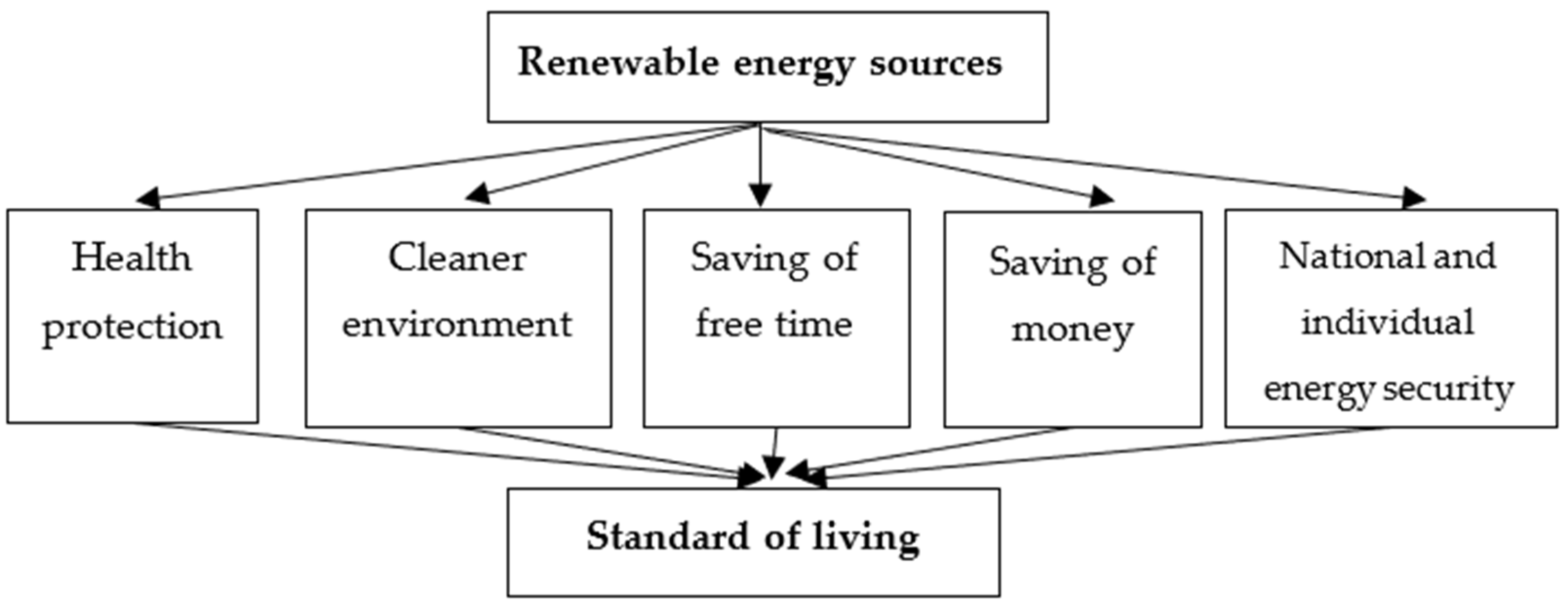
• social-the creation of new workplaces; improvement of residents’ standard of living.
• environmental-improvement in the condition of the natural environment and reduction of greenhouse gas emissions, which will have an impact on limiting the extraction of fossil fuels and, as a result, decreasing environmental burden related to the exploitation of deposits and will reduce the risk of natural disasters.

M. Wozniak and B. Saj point out that energy generated from renewable sources makes it possible to [39]: diversify the available energy sources, create active prosumer attitudes concerning the use of renewable energy in the general energy system of a given country, manage fossil fuels in a reasonable way, obtain relatively cheap, renewable electricity; significantly reduce the negative impact on the environment; reduce the costs related to energy transfer; increase social awareness in terms of ecology; improve the stability of energy supplies (especially in rural areas); expand the entrepreneurial attitudes of residents.

In the context of identifying economic benefits, it is important to assess the profitability of investments in renewable energy sources, for which mainly methods based on cash flow (static and dynamic) are used. Statistical methods used in this regard are pay-back period and rate of return. The pay-back period of the investment in RES is the time after which the revenues cover the expenses. For any investor, a higher level of investment evaluation is when the time is as short as possible. On the other hand, the rate of return of investment outlays in RES is determined based on the relation of revenues obtained as a result of the investment and the amount of the capital employed. The most often used dynamic methods to assess the cost-efficiency of the investment include the net present value (NVP), the internal return rate (IRR) and the modified internal return rate (MIRR). It is often difficult to assess the profitability of investments in the market of energy obtained from renewable sources, due to limitations associated with the lack of complete information on the current and, especially, the future operation of this market, and, in particular, the lack of sufficient information on financial forecasts, future CO2 emission costs and, most importantly, the direction of changes or stability of the existing legislation [42].

Without much reservation, it can be assumed that the main argument for the use of green energy is the prevention of environmental changes and that it is of particular importance in the context of air pollution reduction and prevention of global warming. Global warming changes the environment, increasing the frequency and intensity of extreme weather events.

In 2017, weather-related disasters caused record economic losses, amounting to EUR 283 billion. The European Commission predicts that by the year 2100, such a disaster could affect approximately two-thirds of the population of Europe, while only 5% of the population is affected by them these days. For example, annual damage from river flooding in Europe could rise to EUR 112 billion from the current EUR 5 billion. It is estimated that reduction in predicted food availability with global warming by 2 °C is more significant than with global warming of 1.5 °C (as per the “aim of the Paris Agreement”), including the regions of key importance for the safety of the EU, such as Northern Africa and the rest of the Mediterranean. It could undermine security and prosperity in the broadest sense, harming the economic, food, aquatic and energy system, which would, in turn, cause conflicts and migration pressures [43].

From the perspective of these considerations, it is worth mentioning at this point that the most important negative health effects resulting from air pollution (reflected in the standard of living) include [44]: problems with memory and concentration, depression, anatomical changes in the brain, accelerated ageing of the nervous system, stroke; breathing problems, cough, runny nose, sinusitis; myocardial infarction, hypertension, ischaemic heart disease, cardiac arrhythmias, heart failure; exacerbation of asthma, lung cancer, exacerbation of chronic obstructive pulmonary heart disease, more frequent respiratory infections; low birth weight, missed abortion, premature birth.

At this point, it is also worth mentioning the results of studies conducted by M. Szyszkowicz et al. [45] which show that there is a statistically significant correlation between air pollution with carbon monoxide, sulphur dioxide, nitrogen dioxide and the number of suicide attempts in Vancouver. It has been empirically proven that air pollution is associated not only with respiratory problems but also with depression, anatomical changes in the brain, accelerated ageing of the nervous system, the likelihood of stroke, missed abortion. According to the report by the Jagiellonian University, approx. 44,000 in Poland, one of the infamous European leaders in the level of air pollution, die due to air pollution every year [46]. In its 2015 report Economic Cost of the Health Impact of Air Pollution in Europe, the World Health Organisation states that the estimated economic cost of deaths occurring in Europe as a result of environmental pollution is approximately USD 1.6 trillion per year [47].

According to the BP Energy Outlook 2020 report, there is a clear upward trend in energy consumption all over the world, which leads to many environmental threats. The report shows that oil and coal continue to be the basic source of energy (the trend, however, is downward), and the share of renewable energy sources has been increasing for another year in a row [1].

As M. Tomala [48] correctly observes, renewable energy frequently still turns out to be more expensive than the traditional one, but the use of ecological energy must be based on a high level of social awareness consisting in the understanding of the fact that the wealth of a country does not depend solely on the accumulated capital, but also on the standard of living (as it is in the Nordic countries).

It seems that the cost of investment and operating costs of an energy or heat/cold source remains the most important criterion for the selection of energy production technology. Technologies using renewable energy sources require a relatively large initial investment, but the cost of their ongoing operation is low (solar, wind, water energy). From the perspective of these considerations, an important thing is that lower prices of renewable energy will increase the fund of free decisions of consumers, who will be able to spend the money saved on energy bills on products and services. For this reason, apart from the direct costs of financial investments in RES, we should also take into account the benefits stemming from the use of renewable resources, which to a greater or lesser extent also affect the standard of living of residents (Figure 1).

The amount of the initial capital investment has a large impact on the economic competitiveness of a given technology, especially when estimating the LCOE coefficient (levelized cost of energy). Due to the need for large expenditures at the beginning of the operation, renewable energy sources, especially those using solar technologies, frequently have a higher LCOE coefficient than conventional technologies. This argument is frequently put forward to prove that the use of renewable energy sources is too expensive. Even though the comparison of costs of energy production from renewable and conventional sources depends on the location and conditions in a given country, the LCOE coefficient suggests that using renewable energy sources we can already offer energy services at a competitive price. Moreover, it is believed that technological advancement and greater efficiency will further increase the price competitiveness of all types of RES, compared to conventional technologies. For example, it is assumed that the LCOE coefficient for wind and solar energy will have decreased by 35% (by 2030) and 50% (by 2050), respectively [33].

M. Iganrska observes that the development of the RES sector has a positive impact on the labour market, thus determining the standard of living of residents. This is especially true for the industries manufacturing renewable energy and construction equipment, due to an increase in the demand for construction services related to the construction of power generating facilities and modernization of the existing ones. Employment can also be expected to increase in the banking sector, due to the expansion of programmes financing green energy investments. There will be a shift of human capital from traditional to highly innovative sectors, which will consequently contribute to the development of the knowledge-based economy [49].

Areas allocated for RES investments do not lose their tourist and utility value. Such investments can also result in other types of investments. The areas where RES investments are implemented are perceived as investor-friendly regions, fostering the development of new technologies and protecting the environment, which makes them worth investing in [50].

In the context of the use of renewable energy sources and their impact on the standard of living of residents, it is worth mentioning the change in the time needed for the operation of thermal energy source. In general, taking into account the operation time, we can distinguish two groups of thermal energy sources unmanned sources (such as oil and gas boilers, heat pumps, solar collectors and electric heating) and sources requiring constant maintenance (all kinds of solid fuel and biomass boilers). Their time-consuming nature is dependent and can vary. In the case of changing the power source from group one to group two, the time needed for service will increase, thus generating costs of lost free time. Switching from group one to group two, however, will bring benefits associated with saving free time. Changing an individual source of thermal energy production may be associated with changes in the time needed for the operation of the source. The time needed for the following should be particularly taken into account: operation of the source producing thermal energy (supplying the source with fuel as well as other operation-related activities) during and outside the heating season; fuel management on the property (for example reloading the imported fuel from the storage area) [51].

3. Materials and Methods

All 27 member states of the European Union were included in the empirical analysis. The aim of the analysis was not to compare national fuel resources in individual countries, the structure of energy production by the source, or the share of renewable energy in electricity production as it is the subject of many widely available scientific analyses and reports (more in REN21 [52], bp Statistical Review of World Energy [53], IRENA—RENEWABLE CAPACITY STATISTICS [54]). The author aimed to construct original, synthetic measures of the standard of living and the level of renewable energy development and, on the basis thereof, conduct an assessment of development diversification in the countries of the EU as well as use an advanced, multivariate exploratory technique, i.e., canonical analysis, to assess the correlations between them.

In the literature, the problem of the impact of renewable energy on the life situation of residents was most often analysed in the context of energy poverty—a situation when a household cannot afford energy or energy services to satisfy their basic, daily needs.” Less frequently renewable energy is strictly treated as a livelihood enabler. The use of renewable energy as a tool that eliminates energy poverty and, consequently, contributes to improving the standard of living was emphasized by, among others, C.W. Njiru and S.C. Letema [5] who demonstrated that energy poverty has an impact on the physical health, well-being and welfare of the people living in the Kirinyaga province, Kenya. Similar studies were conducted by E.M. Getie [6] conducted similar studies which revealed that energy poverty has a direct or indirect impact on the standard of living of people in Ethiopia (including human resource development, residents’ health and agricultural automation which improve the standard of living). M.A. Hussein and W.L. Filho [7] analysed the quantitative relationship between energy availability and improved living conditions and elimination of poverty in sub-Saharan Africa. According to the authors, renewable energy technologies play a special role in the improvement of access to energy services for poor people and isolated rural communities. At this point, it is also worth mentioning a study that investigated the relationship between the level of economic development and renewable energy. M. Simionescu et al. [55] showed that there was a potential relationship between the share of renewable energy sources in total electricity and the real GDP per capita. Based on the constructed models for panel data, the authors indicated that GDP per capita had a positive, but very low impact on the share of RES in electricity in the years 2007–2017 in EU countries, except for Luxembourg. On the other hand, based on data from 1992–2018, J. Grabara et al. [56] analysed the relationships between economic growth and the use of renewable energy consumption and direct foreign investments in Kazakhstan and Uzbekistan. Based on the results of the Granger causality test it was, among other things, demonstrated that there is a relationship between direct foreign investments and the use of renewable energy in the countries under consideration. Based on a very extensive literature review of the problem, C. Llamosas and B.K. Sovacool [57] indicate numerous benefits resulting from the construction and operation of transboundary dams. According to them, the economic benefits include the possibility of exporting electricity, effectively generating income for hydropower exporters, while the catalytic benefits include knowledge transfer, as well as building confidence and industry experience.

An initial determination of variables describing the analysed objects (EU countries) constituted the first stage of constructing synthetic measures of EU residents’ standard of living and the level of the development of renewable energy sources (a kind of “green energy index”), according to the multivariate analysis. Both in the case of the quantification of the standard of living and the level of renewable energy development, the variables should be selected in such a way so as to reflect various aspects of these multivariate categories. As M. Walesiak correctly observes, the selection of variables is among the most important and most difficult issues. This is because the quality of variables determines the reliability of the final classification results and the accuracy of the decisions made on their basis. Only the variables which can discriminate a set of objects should be included in the classification procedure [58].

On the one hand, issues related to the assessment of the standard of living (and the quantification of environmental aspects, including those related to renewable energy) enjoy a great interest of researchers, but on the other—they are controversial. This is largely due to the multifaceted and interdisciplinary nature of this research category, which fosters the emergence of various measures and indicators relating to this phenomenon. No single, universally accepted method of measuring the standard of living of residents has been developed to date. To illustrate, at least partially, the results of works on the construction of synthetic measures obtained so far, listed below are those which in the author’s opinion are most popular in the literature in the context of the assessment of the living standard (and related categories, such as the quality of life or living conditions) and the degree of sustainability of socio-economic development (“greening of the economy” (including the use of renewable energy sources), the level of sustainable development):

• Index of the Economic Aspects of Welfare (EAW) is one of the first measures of economic welfare to more broadly incorporate the ecological aspect and a broad spectrum of qualitative factors. It was applied for the first time by X. Zolotas in 1981. Its structure is focused on the current flow of goods and services. It takes into account expenditures on public buildings, the value of household works, expenditures on durable consumer goods, advertising, the value of free time, the value of public sector services, corrected by the expenditures related to health care and education, costs of environmental pollution and the depletion of natural resources [59,60].
• Index of Sustainable Welfare (ISEW), developed in 1989 by H. Daly and J. Cobb. The first step in the construction of this measure is the correction of personal expenditures of a population by the income index spread. The obtained values are then modified by adding or subtracting monetary values of a predetermined set of factors (of social, economic and environmental nature), depending on whether a given factor has a positive or negative impact on welfare. Expenditures related to, among other things, public education and health care, or the value of services from domestic work, increase the base value and decrease, among other things, the costs of commuting, unemployment and natural environment exploitation as well as crime-related costs [61,62].
• Human Development Index (HDI), which is a complex measure based on the geometric mean of three (normalized) indicators relating to basic dimensions of human life: the ability to live a long and healthy life, measured by life expectancy at birth; the ability to acquire knowledge, measured by average years of education and the expected years of education; and the ability to attain a decent standard of living, measured by gross income per capita. Since 1900, the index has been recurrently published as part of the Human Development Report prepared by the UN Development Programme [63].
• Multidimensional Poverty Index (MPI), which replaced the HPI (Human Poverty Index) index applied since 1997. It comprises 10 elements aggregated into 3 dimensions [64]: I. Education (1. no household member has been receiving education for at least 6 years); 2. no school-age child is attending school); II. Health (1. at least one household member is malnourished; 2. child mortality); III. Living conditions (1. lack of access to electricity; 2. lack of access to clean drinking water; 3. lack of access to sanitary facilities; 4. use of “dirty cooking fuel” (e.g., charcoal); 5. disorder in the household; 6. owning at least one asset related to access to information (radio, television, telephone), mobility or supporting the household (fridge, arable land, livestock).
• Quality of Life Index (QoL), an indicator developed by “The Economist” and used for the first time in 2005 for 111 countries. The indicator is based on a unique methodology combining the results of subjective satisfaction with life and an examination of objective determinants of the quality of life. The following parameters are taken into account while calculating the index: financial situation, political stability and safety, family life (divorce rate per 1000 residents), community life (the rate of church attendance or trade union membership), climate and geography, job security (unemployment rate), political freedom, gender equality (the ratio of average earnings of men and women) [65].
• Better Life Index (BLI), created in 2011 by OECD for international comparison of social welfare. The index consists of 11 parameters: income and wealth (corrected net disposable income of a household, net household assets), work and remuneration (employment rate, long-term unemployment rate, average gross earnings of full-time employees, uncertainty in the labour market), housing (number of rooms per person, houses without basic amenities, housing expenditures), health (average life expectancy at birth, self-reported health), life and work (employees spending long hours at work (more than 50 h per week), time for leisure and personal care), education and skills (level of education, cognitive skills of students, expected years of education), social bonds (support in social media), civic involvement (participation in the development of legislation, voter turnout), quality of the natural environment (air pollution, satisfaction with water quality), personal security (homicide rates, the sense of safety while walking alone), satisfaction with life [66].
• The Happy Planet Index (HPI) was developed by the New Economics Foundation. It is used to measure the well-being in specific countries and is the product of the life expectancy and the citizens’ general satisfaction with life, as well as a measure reflecting the uneven distribution of life expectancy and the well-being experienced in a given country, divided by the so-called ecological footprint, i.e., the use of the natural environment [67].
• The Social Progress Index (SPI) is constructed based on 50 variables concerning 12 components, which are grouped into three categories: basic human needs, foundations of well-being and opportunity: nutrition and basic medical care, air, water and sanitation, shelter and personal safety (included in the 1st category), access to basic knowledge, access to information and communication, health and well-being, environmental quality (included in the 2nd category), personal rights, personal freedom and choice, inclusiveness and access to advanced education (included in the 3rd category) [68].

Among synthetic measures more focused on the environmental aspects, the following are worth mentioning:

• Living Planet Index (LPI), an index promoted by the Word Wildlife Foundation, measuring biological diversity based on data on various species of vertebrae and calculating the average change in their number over time. The measurement aims to identify biodiversity threatened by human activity. The situation of the analysed populations is compared with the situation observed in 1970 [69].
• Ecological Footprint, used as a measure of human demand for broadly defined natural capital. The “Ecological Footprint” determines how many biologically productive land and sea areas are necessary to provide resources for consumption and absorb the generated waste, based on the existing technological solutions combined with specific resource management practices [70].
• Global Green Economy Index (GGEI)—developed in 2010 r. by Dual Citizens Inc. as a complex analytical tool offering stakeholders a system for improving their operation and image within the framework of “green economy”. In 2018, its structure was based on 20 partial indicators relating to four main thematic areas: leadership in green economy implementation (actions of public entities, managements, creation of institutions, international cooperation) and climate changes; effectiveness sectors (including construction, transport and energy); markets and investments; environment [71].

According to J. Piasny [22], synthetic measures, rather than partial indicators, are a more appropriate measure of the inhabitants’ standard of living. However, some limitations on the use of synthetic measures should be kept in mind [72]: subjective selection of diagnostic variables used for the construction of a synthetics measure; subjective selection of weights for individual variables in the aggregation formula.

Considering the limited availability of statistical data, it is difficult to conduct a complex measurement of the standard of living, because the level of this multifaceted phenomenon is determined by the level of satisfaction of the above-described needs, both material and non-material. In the context of multidimensional phenomena, K. Nermend [73] indicates what, in terms of content and form, the analysed variables should be characterised by, which includes capturing the most important properties of studied phenomena, being precisely defined, logically interrelated, measurable (directly or indirectly), expressed in natural units (in the form of intensity indicators), containing a significant information load, and being characterised by high spatial variability.

The procedure of diagnostic variable selection consisted of two stages (both in the case of variables related to the standard of living and renewable energy). In the first stage, a set of potential diagnostic variables was proposed based on the above-listed formal and substantive premises (the data was obtained from the EUROSTAT database—

Table A1. Data on the standard of living—part 1.

	S1	S2	S3	S4	S5	S6	S7	S8	S9	S10	S11	S12	S13	S14	S15	S16
Belgium	81.70	5.80	377.30	3.80	1.62	29.00	39.29	12.80	37.42	1.00	47.50	24193.00	41450.00	2.30	69.00	5.40
Bulgaria	75.00	−7.00	63.40	5.80	1.56	26.20	31.55	17.50	28.65	1.00	32.50	7051.00	8780.00	2.40	73.20	4.20
Czechia	79.10	4.10	138.20	2.60	1.71	28.40	34.40	13.20	37.41	1.00	35.10	11996.00	20990.00	0.60	76.70	2.00
Denmark	81.00	2.90	138.50	3.70	1.73	29.50	30.68	10.00	41.41	1.00	49.00	33932.00	53760.00	0.80	79.10	5.00
Germany	81.00	1.80	235.20	3.20	1.57	29.70	28.41	9.30	54.50	1.00	35.50	26128.00	41510.00	1.20	79.20	3.10
Estonia	78.50	3.10	30.50	1.60	1.67	27.70	50.60	11.60	29.65	1.00	46.20	13193.00	21220.00	0.90	78.90	4.40
Ireland	82.30	12.20	71.90	2.90	1.75	30.50	25.06	12.60	48.24	1.00	55.40	32644.00	72260.00	1.60	73.30	5.00
Greece	81.90	−0.60	82.40	3.50	1.35	30.40	14.16	20.70	30.15	1.00	43.10	10068.00	17110.00	12.20	68.40	17.30
Spain	83.50	8.40	93.80	2.70	1.26	31.00	27.61	16.00	35.42	1.00	44.70	19135.00	26430.00	5.30	73.80	14.10
France	82.90	2.10	106.10	3.80	1.88	28.70	37.86	14.00	50.30	1.00	47.50	27062.00	35960.00	3.40	71.70	8.50
Croatia	78.20	−4.40	72.80	4.20	1.47	28.80	28.10	15.00	42.81	1.00	33.10	9227.00	13340.00	2.40	66.50	6.60
Italy	83.40	−2.90	201.50	2.80	1.29	31.20	24.71	23.80	29.42	1.00	27.60	20570.00	29660.00	5.60	65.70	10.00
Cyprus	82.90	13.70	95.70	2.40	1.32	29.80	27.97	14.60	30.63	1.00	58.80	21492.00	25310.00	2.10	76.00	7.10
Latvia	75.10	−6.40	30.20	3.20	1.60	27.20	40.31	12.00	29.43	1.00	45.70	10852.00	15920.00	2.40	77.30	6.30
Lithuania	76.00	0.00	44.60	3.40	1.63	27.80	37.01	11.60	58.82	1.00	57.80	10871.00	17460.00	1.90	78.00	6.30
Luxembourg	82.30	19.70	239.80	4.30	1.38	30.90	28.64	6.90	36.58	1.00	56.20	48452.00	102200.00	1.30	72.00	5.60
Hungary	76.20	−0.30	107.10	3.30	1.55	28.20	31.83	14.60	40.09	1.00	33.40	7458.00	14950.00	1.10	72.60	3.40
Malta	82.50	41.70	1595.10	5.60	1.23	29.20	19.10	9.60	25.89	1.00	38.10	17290.00	26670.00	0.90	75.90	3.60
Netherlands	81.90	7.20	507.30	3.50	1.59	30.00	27.49	7.00	46.43	1.00	51.40	27213.00	46710.00	1.00	80.90	3.40
Austria	81.80	4.80	107.60	2.70	1.47	29.50	29.04	9.20	38.52	1.00	42.40	28094.00	44780.00	1.10	77.10	4.50
Poland	77.70	−0.40	123.60	3.80	1.46	27.40	35.85	13.40	29.04	1.00	46.60	9317.00	13870.00	0.70	70.60	3.30
Portugal	81.50	1.90	113.00	3.30	1.42	29.80	23.38	9.50	35.62	1.00	36.20	12962.00	20740.00	2.80	75.50	6.50
Romania	75.30	−4.40	82.70	6.00	1.76	26.70	26.84	17.30	37.60	1.00	25.80	6196.00	11510.00	1.70	68.60	3.90
Slovenia	81.50	7.20	103.70	1.70	1.60	28.80	29.15	9.00	26.21	1.00	44.90	16048.00	23170.00	1.90	75.20	4.50
Slovakia	77.40	1.40	112.00	5.00	1.54	27.10	30.51	17.20	46.64	1.00	40.10	9869.00	17210.00	3.40	72.70	5.80
Finland	81.80	1.30	18.20	2.10	1.41	29.20	37.76	10.30	32.89	1.00	47.30	30065.00	43570.00	1.20	78.30	6.70
Sweden	82.60	9.50	25.20	2.00	1.76	29.30	45.26	6.40	37.37	1.00	52.50	27419.00	46160.00	0.90	82.90	6.80

Source: own study based on [8].

,

Table A2. Data on the standard of living—part 2.

	S17	S18	S19	S20	S21	S22	S23	S24	S25	S26	S27	S28	S29	S30	S31	S32
Belgium	562.24	950.00	312.96	26.10	15.70	1860.06	760.71	46.00	0.84	511.00	57.75	5.10	2.10	22.58	5902.24	15.00
Bulgaria	756.91	735.00	421.71	21.60	32.00	1382.13	588.61	42.10	0.52	396.00	6.86	6.40	1.20	35.15	18535.87	13.10
Czechia	661.82	369.00	403.76	36.20	5.60	2802.33	1043.01	50.90	0.88	540.00	15.87	2.40	1.50	33.92	2621.03	11.10
Denmark	242.97	442.00	419.44	31.30	2.80	3677.02	894.40	48.00	0.21	447.00	30.96	4.60	1.90	14.62	3693.70	8.40
Germany	800.23	6203.00	431.09	43.20	7.10	4188.11	1754.77	45.71	0.61	567.00	36.77	3.50	1.80	31.95	4884.70	25.20
Estonia	457.35	183.00	348.34	44.20	2.40	1956.05	1159.80	48.00	1.07	563.00	3.41	2.20	1.70	53.91	17500.93	10.20
Ireland	297.39	324.00	327.94	27.70	8.10	3322.74	1761.88	54.00	0.53	445.00	13.12	2.20	2.10	11.15	2851.97	6.50
Greece	419.77	1064.00	500.80	23.70	15.60	2202.70	854.44	49.50	3.53	487.00	0.00	5.60	1.20	29.55	4251.22	20.20
Spain	297.15	5374.00	402.08	29.20	7.80	3637.26	1433.42	61.48	1.13	513.00	30.80	2.20	1.90	36.70	2936.34	9.90
France	590.85	4851.00	317.08	38.00	3.00	4623.02	1831.68	50.00	0.44	478.00	18.43	4.20	1.90	27.12	5096.75	14.90
Croatia	561.25	210.00	344.06	36.60	12.40	1730.50	541.05	60.30	27.91	409.00	23.15	5.90	1.10	34.22	1359.91	5.90
Italy	314.05	5901.00	397.71	15.90	28.90	3579.82	1099.60	49.00	3.62	646.00	22.98	5.40	1.40	31.49	2857.92	12.40
Cyprus	330.09	79.00	407.32	38.80	39.40	1156.03	632.05	71.80	0.93	629.00	27.78	0.90	2.00	0.13	2628.32	8.40
Latvia	549.35	191.00	330.38	42.10	27.90	863.75	472.62	43.30	0.64	369.00	0.00	12.40	1.20	52.76	923.83	18.30
Lithuania	643.40	241.00	459.78	36.80	12.30	1719.37	751.48	44.00	1.34	512.00	4.96	5.40	1.60	33.70	2534.03	17.10
Luxembourg	450.70	22.00	298.49	25.10	16.60	566.15	202.22	30.87	0.69	676.00	63.81	3.20	2.00	34.30	14683.96	15.20
Hungary	701.29	470.00	338.37	39.70	12.10	1785.31	745.49	41.90	0.45	373.00	21.31	6.80	1.50	22.09	1879.67	12.40
Malta	430.84	88.00	397.21	30.50	14.40	962.30	407.40	66.20	0.49	608.00	0.00	1.40	2.20	1.46	5079.58	33.90
Netherlands	316.55	1868.00	366.96	32.20	6.20	4148.33	1492.09	50.20	0.51	494.00	66.35	1.70	2.00	8.87	8404.10	14.90
Austria	727.16	701.00	524.14	37.40	5.40	4120.70	1508.01	48.00	2.48	562.00	20.78	5.80	1.60	46.44	7412.55	10.50
Poland	653.69	1677.00	237.75	39.20	23.40	1966.12	742.57	41.70	0.30	617.00	5.24	8.10	1.10	30.29	4612.34	13.80
Portugal	344.51	934.00	442.42	41.20	14.80	2530.21	1137.99	51.05	0.70	514.00	33.23	5.40	1.70	35.91	1546.70	13.50
Romania	696.83	814.00	304.70	18.90	13.90	1268.17	546.22	39.72	0.42	332.00	3.45	4.10	1.10	29.07	10466.60	13.50
Slovenia	442.79	67.00	317.81	35.80	5.10	2115.91	733.83	43.99	4.60	549.00	30.73	4.50	1.60	61.16	3950.52	16.20
Slovakia	569.62	124.00	397.34	31.80	13.50	2050.79	707.96	36.16	0.63	426.00	9.83	1.40	1.20	39.28	2275.40	9.50
Finland	361.18	347.00	320.63	49.50	4.50	2906.83	1655.78	41.99	0.25	629.00	2.74	1.00	1.90	66.21	23232.55	9.40
Sweden	213.79	738.00	426.52	36.90	3.70	4613.31	2393.94	45.00	0.43	476.00	4.86	3.60	1.80	63.80	13554.75	6.60

Source: own study based on [8].

and

Table A3. Data on the level of development of renewable energy sources.

	R1	R2	R3	R4	R5	R6	R7	R8	R9	R10	R11
Belgium	0.01	0.07	0.03	0.01	0.01	20.83	8.31	6.81	0.00	66.85	1.18
Bulgaria	0.04	0.02	0.02	0.00	0.00	23.51	35.51	7.89	0.00	60.78	0.09
Czechia	0.03	0.01	0.02	0.02	0.00	14.05	22.65	7.83	0.16	52.11	0.74
Denmark	0.00	0.24	0.01	0.01	0.01	65.35	48.02	7.17	0.00	329.85	0.55
Germany	0.03	0.13	0.05	0.03	0.01	40.82	14.55	7.68	0.08	232.79	0.59
Estonia	0.00	0.04	0.00	0.00	0.00	22.00	52.28	5.15	0.00	0.00	0.06
Ireland	0.02	0.18	0.00	0.00	0.01	36.49	6.32	8.93	0.00	68.71	0.42
Greece	0.03	0.06	0.04	0.00	0.00	31.30	30.19	4.05	0.79	453.86	0.21
Spain	0.05	0.10	0.02	0.00	0.00	36.93	18.87	7.61	0.59	93.95	0.79
France	0.08	0.04	0.02	0.00	0.00	22.38	22.46	9.25	0.87	49.16	0.32
Croatia	0.13	0.03	0.00	0.01	0.00	49.78	36.79	5.86	0.00	66.78	0.09
Italy	0.07	0.03	0.03	0.01	0.00	34.77	19.67	9.05	1.97	71.96	0.36
Cyprus	0.00	0.02	0.02	0.01	0.00	9.76	35.10	3.32	0.00	1237.71	0.16
Latvia	0.09	0.01	0.00	0.02	0.00	53.42	57.76	5.11	0.00	11.29	0.09
Lithuania	0.03	0.05	0.00	0.00	0.00	18.79	47.36	4.05	0.02	0.00	0.28
Luxembourg	0.13	0.04	0.02	0.01	0.01	10.86	8.71	7.66	0.02	112.77	0.46
Hungary	0.00	0.01	0.01	0.00	0.00	9.99	18.12	8.03	0.01	35.81	0.19
Malta	0.00	0.00	0.04	0.00	0.00	8.04	25.70	8.69	0.00	148.94	0.44
Netherlands	0.00	0.06	0.03	0.00	0.01	18.22	7.08	12.51	0.00	39.98	1.59
Austria	0.43	0.07	0.02	0.01	0.00	75.14	33.80	9.77	0.16	570.10	0.86
Poland	0.01	0.03	0.00	0.00	0.00	14.36	15.98	6.12	0.03	71.00	0.44
Portugal	0.09	0.11	0.01	0.00	0.00	53.77	41.65	9.09	1.02	131.17	0.84
Romania	0.07	0.03	0.01	0.00	0.00	41.71	25.74	7.85	0.00	10.53	0.32
Slovenia	0.19	0.00	0.01	0.00	0.00	32.63	32.16	7.98	0.00	107.80	0.36
Slovakia	0.07	0.00	0.01	0.01	0.00	21.95	19.70	8.31	0.13	0.00	0.48
Finland	0.19	0.09	0.00	0.01	0.01	38.07	57.49	21.29	0.00	13.23	1.86
Sweden	0.55	0.17	0.01	0.00	0.01	71.19	66.12	30.31	0.47	44.87	0.66

Source: own study based on [8].

). The selection primary of sets of variables, apart from the substantive and formal criteria, was largely determined by the availability, completeness and the fact that this data is up-to-date. It was assumed that the included partial variables will be indicative and will not be absolute values, which was aimed at eliminating the distortion related to the fact that some objects (EU countries) have some characteristic traits (eg. a significantly larger area than other objects).

As a result, 29 potential diagnostic variables related to the standard of living were proposed. The variables were then divided according to substantive criteria into seven thematic groups [9,13,74,75]:

• demography: S1—Average life expectancy at birth; S2—The birth rate; S3—Population density; S4—Infant mortality rate; S5—Total birth rate. S6—Average age of mothers at birth.
• education: S7—Students enrolled in early childhood education (pre-school education) per 1000 inhabitants; S8—Percentage of young people not working or studying (aged 15–24); S9—Percentage of university students in relation to the population S10—Percentage of people with higher education in the age group 25–64 (variables S9 and S10 are similar, however, it is assumed that not every student completes his/her studies and obtains higher education).
• economy and labour market: S11—average remuneration; S12—gross domestic product in market prices per person; S13—long-term unemployment rate (12 months and more); S14—professional activity rate (age 15–74); S15—unemployment rate, S16—the percentage of people at risk of poverty and social exclusion.
• health: S17—available beds in hospitals (per 100,000 residents); S18—doctors (per 100,000 residents), S19—the percentage of people with chronic illnesses or health problems,
• tourism: S20—nights spent at tourist accommodation establishments (per 1000 residents); arrivals at tourist accommodation establishments (per 1,000 residents); S22—net occupancy of beds and rooms in hotels and similar establishments;
• transport: S23—cars per 1000 residents; S24—length of highways per 100 km²;
• housing conditions: S25—level of severe housing deprivation; S26—the average number of rooms per person,
• environmental protection: S27—forestation rate, S28—dangerous waste production (in tonnes per person); S29—the percentage of people exposed to pollution or other environmental problems.
• In turn, a set of 11 diagnostic variables, divided into two thematic groups, was used to determine the level of renewable energy development in individual EU countries.
• RES production: R1—production of electricity and derived heat based on hydroenergy (in TOE per 1000 residents); R2—production of electricity and derived heat based on wind energy (in TOE per 1000 residents); R3—production of electricity and derived heat based on photovoltaic energy (in TOE per 1000 residents), R4—production of electricity and derived heat based on biogas fuels (in TOE per 1000 residents) R5—production of electricity and derived heat based on communal waste (in TOE per 1000 residents), R6—share of energy from renewable sources in final electricity consumption, R7—share of energy from renewable energy sources in energy used for heating and cooling, R8—share of energy from renewable sources in energy used in transport,
• RES infrastructure: R9—installed heat pump capacity (in megawatts per 1000 residents), R10—solar collector surface (in km² per 1000 residents), R11—“autoproducers” of electricity from renewable energy sources per 1000 residents.

The multitude of variables (being carriers of various information) describing the analysed objects in multidimensional comparative analyses makes it necessary to choose the most important ones from the research point of view. Therefore, at the second stage of variable selection, to limit the number of potential diagnostic variables, statistical procedures were used so that the selected variables characterized the studied objects as fully as possible and, simultaneously, created a set as small as possible. As M. Walesiak [58] correctly observes, the approach which is to take account of as many variables as possible is unsubstantiated as adding one or several irrelevant variables to the set makes it impossible to detect the proper structure in the set of objects.

Studying variability and the degree of correlation of potential diagnostic data (information criterion) is of particular importance in the process of variable selection.

During variable selection, it is required that individual observations exhibit adequate variability (discriminatory ability) as poorly varied variables provide little analytical value. It was assumed that those traits will be eliminated from both primary sets for which the absolute value of classic variability coefficient will be below the arbitrarily determined, critical threshold value of this coefficient at the level of 10% (the traits were considered quasi-constant, not bringing significant information on the studied phenomenon). Subsequently, the degree of variable correlation (information capacity) was investigated, since it is assumed that two highly correlated variables are carriers of similar information, which makes one of them redundant. For this reason, in order to conduct information value assessment, one of the methods of feature discrimination depending on the value of correlation matrix—the so-called method of inverse correlation matrix—was used (more in: [76]). Based on the correlation matrix, the inverse correlation matrix was calculated for each thematic variable subgroup

$$R^{-1}=\left[{\tilde{r}}_{jj},\right]j,j\prime =1,2,\dots ,m, \mathrm{where}:$$

(1)

${\tilde{r}}_{j{j}^{\prime }}=\frac{{\left(-1\right)}^{j+j\prime }\left|R_{jj\prime }\right|}{\left|R\right|}$, where: $R_{j{j}^{\prime }}$—the matrix reduced by deleting the j-th row and the j’-th column; $R, \left|R_{jj\prime }\right|$—determinants of the R and Rjj′ matrices respectively.

In features that are overly correlated with other diagonal elements of the inverse correlation matrix are much greater than 1 (which means that the matrix is ill-conditioned). According to this method, the overly correlated feature (which corresponds to the diagonal element of the inverse correlation matrix characterized by the value exceeding the arbitrarily determined threshold value (most often r* = 10) is eliminated from the primary set of features. Then the inverse correlation matrix is calculated again, and it is analysed whether the diagonal values do not exceed the determined threshold value. The procedure is continued until all diagonal values not exceeding the determined threshold are obtained (i.e., until the stability of the inverse correlation matrix is achieved).

As a consequence, taking into account the discriminatory criterion, 4 variables (S1, S6, S9, S14) should be eliminated from the set of variables relating to the standard of living. On the other hand, all variables in the set of variables relating to the level of renewable energy development were characterized by a variable coefficient greater than the adopted critical threshold of 10%. For this reason, all variables in this set were further analysed. After conducting the assessment of the information potential (based on the results obtained with the use of the inverse correlation method) variables R4, R7 and R11 were eliminated from the set describing the level of renewable energy development, while variables S12 and S29 were eliminated from the set relating to the standard of living.

In studies aimed at linear ordering of a set of objects, variable classification by preferences among variables is of particular significance. In this context, we distinguish stimuli (high values desired from the perspective of the essence of the phenomenon under consideration), dampers (desired low values) and neutral variables (where certain nominal values constitute the optimal value, and deviations from the value worsen the evaluation of the analysed phenomenon). In the set of data relating to the standard of living, the following variables were included in the damper set: S3 (population density); S4 (infant mortality rate); S8 (young people not in employment and not attending any school (age 15–24)); S13 long-term unemployment rate (12 months and above) and S15 (unemployment rate); S16 (percentage of people at risk of poverty and social exclusion); S19 (percentage of people with chronic diseases or health problems); S25 (degree of significant housing deprivation); S28 (production of dangerous waste). The other variables were treated as stimuli. This also applies to the variables describing the sphere of tourism, assuming that the higher values of considered variables, the greater the tourist attractiveness and the more opportunities for leisure activities. In the set of variables relating to the level of renewable energy development, all variables under consideration were classified as stimuli.

In studies using linear ordering and classification methods, there is a need to de-value variables and standardise orders of magnitude to render them comparable. This operation is known as normalization transformation. The most common methods of data normalization include standardization, unitization and quotient transformation. Normalisation was performed by standardizing the value of a variable. The purpose of standardisation is to obtain variables with a distribution with an average of 0 and a standard deviation of 1. On the other hand, the most popular [58,77] standardization formula has the form:

$$z_{ij}=\frac{x_{ij-{\overline{x}}_j}}{S_j}$$

(2)

where: ${\overline{x}}_j$—arithmetic mean; S_j—standard deviation of variable x_ij; i = 1, 2, ..., n; j = 1, 2, ..., m.

The so selected and initially transformed set of values, became the basis for linear ordering of the considered objects (as well as further analyses). The classic TOPSIS (the Technique for Order of Preference by Similarity to Ideal Solution) method, which is considered to be a model method, was used to facilitate linear ordering of the selected countries of the European Union in terms of the standard of living of the residents and the level of renewable energy development. This method makes it possible to determine the hierarchy of objects in accordance with the adopted criteria. It is a certain modification of Hellwig’s method, which is popular among scientists. In this method, the synthetic measure is constructed taking into account the Euclidean distance of observation not only to the pattern (the most desired variant) but also from the anti-pattern, known as the anti-deal reference solution (in contrast to Hellwig’s method, in the case of which only the distance from the patter is considered). The following stages in the construction of a synthetic measure can be distinguished in this method [78]:

• Creating a standardized decision matrix based on the quotient transformation.

  $$z_{ij}=\frac{x_{ij}}{\sqrt{{\sum }_{i=1}^m{x}_{ij}^2 }} \mathrm{for} i = 1, 2,\dots m \mathrm{and} j = 1, 2, \dots , m$$

  (3)

  where: x_ij —the observation of the j-th variable in the i-th object.

• Constructing a matrix of weights using weighing of variables and subsequently creating a weighted standardized decision matrix (as a result of multiplying the standardized values by the weights):

$$v_{ij}=w_j· z_{ij}$$

(4)

• Based on the standardized decision matrix, the value vector for the pattern (A⁺) and the anti-pattern (A⁻) is determined:

$$A^{+}=\begin{array}{c}(\max \left(v_{i1}\right), \\ i\end{array}\begin{array}{c}\max \left(v_{i2}\right)\\ i\end{array},\dots ,\begin{array}{c}\max \left(v_{iN}\right))\\ i\end{array}=\left(v_1^{+},v_2^{+},\dots , v_n^{+}\right),$$

(5)

$$A^{-}=\begin{array}{c}(\min \left(v_{i1}\right),\\ i\end{array}\begin{array}{c} \min \left(v_{i2}\right)\\ i\end{array},\dots ,\begin{array}{c}\min \left(v_{iN}\right))\\ i\end{array}=\left(v_1^{-},v_2^{-},\dots , v_n^{-}\right),$$

(6)

• Indicating the distance from the pattern and the anti-pattern for each analysed object based on the Euclidean metric:

$$s_i^{+}=\sqrt{{\sum }_{j=1}^N{\left(v_{ij}-v_j^{+}\right)}^2; } s_i^{-}=\sqrt{{\sum }_{j=1}^N{\left(v_{ij}-v_j^{-}\right)}^2}, i=1,2,\dots , M, j=1,2,\dots ., N$$

(7)

• Determining the value of the synthetic variable which defines the similarity of objects to the “model” solution, in accordance with the following formula:

$$C_i=\frac{s_i^{-}}{s_i^{+}-s_i^{-}}, \mathrm{where} 0\le C_i\le 1$$

(8)

The smaller the distance of a given object from the model unit and, therefore, the greater the development anti-pattern, the closer the value of the synthetic feature to 1.

A classification of the EU countries by the standard of living of their residents and the level of renewable energy development was conducted with the use of the PAM (Partitioning Around Medoids) method to determine groups of objects similar to each other in terms of variables describing them. As correctly observed by J. Korol and P. Szczuciński [79], classification methods make it possible to divide the analysed object sets into adequate subsets (classes) in such a way that the objects belonging to the same subset are most similar to each other, while those belonging to different subsets are least similar to each other. The idea behind clustering methods is to delimit a set of objects into homogenous subgroups, enabling better description thereof from the perspective of the purpose of structural comparisons.

The PAM method is among relatively new classification methods (the mechanism of clustering around medoids was proposed by Kaufman and Rousseeuw in 1987) (more in: [80,81]). The idea behind this method is to search for k objects, so-called representatives, which are centrally located in clusters (so-called medoids). An object in which the mean dissimilarity (distance to the representative) of all objects in the cluster is the smallest is considered to be the representative of the cluster. In reality, the algorithm minimizes the sum of dissimilarities instead of the mean dissimilarity. The selection of k medoids is a process consisting of two steps. First, an initial clustering is obtained by successive selection of “representative” objects until k objects are checked. The first object is the one for which the sum of dissimilarities for all other object is as small as possible (it is a certain kind of a “multidimensional median” of N objects, hence the term “medoid). In each subsequent step, the object which to the greatest extent contributes to the decreasing of the objective function (the sum of dissimilarity) is selected. The next stage is a sort of attempt to correct the set of representatives. It is done by including all pairs of objects (i, h) for which i object was selected for the set of representatives, and an h object does not belong to the set of representatives, checking whether after changing the i into the h, the objective function decreases. The final mean distance (dissimilarity), which is interpreted as the measure of the “goodness” of the final clustering of the considered objects, is expressed by the following formula:

$$F=\frac{{\sum }_{i=1}^N{d}_{i,m\left(i\right)}}{N}$$

(9)

where: m(i) is the representative (medoid) of the closest i object.

Two types of isolated clusters can be distinguished in the algorithm of this method: the L-cluster and the L*-cluster. The C cluster is an L-cluster if the following condition is met for each i object belonging to C:

$$\begin{array}{c}max\\ j\in C\end{array} d_{ij}< \begin{array}{c}min\\ h\notin C\end{array} d_{ih}.$$

(10)

In turn, the C cluster is an L*-cluster if:

$$\begin{array}{c}max\\ i,j\in C\end{array} d_{ij}< \begin{array}{c}min\\ l\in C, h\notin C\end{array} d_{lh}.$$

(11)

The diameter of the C cluster, defined as the greatest dissimilarity (distance) between the objects belonging to C, is determined in this method:

$$D_C=\begin{array}{c}max\\ i,j\in C \end{array}{d}_{ij}$$

(12)

When j is the medoid of the C cluster, the mean distance from the considered C objects to j is calculated as follows:

$${\overline{d}}_j=\frac{{\sum }_{i\in C}{d}_{ij}}{N_j}$$

(13)

In addition, the maximum distance of all C objects to j is calculated as follows:

$$DIS{T}_{max}=\begin{array}{c}max\\ i\in C\end{array} d_{ij}$$

(14)

It was arbitrarily assumed that there would be 4 clusters.

Subsequently, a canonical analysis was conducted to present multidimensional correlations between the sets of variables relating to the standard of living of EU residents and the level of renewable energy development. Canonical analysis can be viewed as a generalization of the linear multiple regression (in which the variability of one endogenous variable may be explained by the variability of a set of exogenous variables) into two sets of variables (endogenous and exogenous). If the set of response features consists of only one feature, the method is equivalent to multiple regression. Therefore, canonical analysis searches for an answer to the question of what is the extent of the simultaneous influence of the whole set of endogenous variables on the whole set of exogenous variables. Analysis of correlations between two sets of variables comes down to analysing the relationships between two new types of variables (so-called canonical variables, also known as canonical roots). Canonical roots constitute the weighted sums of the first and second primary data sets. The weights are generated in a manner that maximizes the mutual correlation of the weighted sums. If this condition is met, it means that pairs of canonical variables are considered to be good representations of the initial data within the framework of the adopted model. Maximum correlation is sought with the use of the Lagrange multiplier method (see: [82,83,84,85,86,87]). Considering the arrangement of two random variables [x, y], where: $x={\left[x_1,x_2,\dots , x_p\right]}^T$ is a vector of exogenous variables, $y={\left[y_1,y_2,\dots , y_q\right]}^T$is a vector of endogenous variables, the aim is to maximize the value of the expression:

$$r_l=\frac{\left(w_x^T{R}_{xy}{w}_y\right)}{\sqrt{\left(w_x^T{R}_{xx}{w}_x{w}_y^T{R}_{yy}{w}_y\right)}},$$

(15)

where: R_xx—the correlation matrix of exogenous variables, R_yy—the correlation matrix of endogenous variables, R_xy—the correlation matrix of both types of variables, w_x, w_y—weights for the first and second type of canonical variables; r_l—the canonical correlation coefficient.

The literature review concerning the application of canonical analysis indicates that this technique remains one of the least commonly used statistical methods in social sciences. Thus, it is also a rarely used tool in the context of the issues of living standards and factors determining the level of this phenomenon. Here, we can mention the studies of O.R. Ebenezer who conducted a canonical analysis which showed that there is a positive correlation between the levels of poverty and literacy concerning data from the state of Ekiti in central Nigeria [88]. In contrast, K. Chin-Tsai [89] conducted a canonical analysis to evaluate correlations between quality of life and professional satisfaction among cyclists. In the context of energy sources, a canonical analysis has been used, for instance, by T. Saeed and G.A. Tularam [90] to identify relationships between fossil fuel prices (oil, natural gas and coal) and climate change (expressed by variables related to green energy, carbon emissions, temperature and precipitation indexes). F.J. Santos-Allamilos et al. [91] used a canonical analysis to assess the spatio-temporal balance between regional resources of solar and wind energy. The conducted analysis indicated the optimal distribution of wind farms and solar power plants throughout the analysed territory (south of the Iberian Peninsula) to minimise the variability of total energy contribution in the power system.

It appears that the relatively low popularity of this tool among researchers and in economic analyses (compared to, for example, classical correlation analysis or regression analysis) may result from at least two reasons. Firstly, the method itself is quite complicated (it requires knowledge of, e.g., multiple regression). Secondly, there are some difficulties in interpreting the obtained results (e.g., a high number of determined indicators). Considering the multifaceted nature of both the standard of living and the level of renewable energy development, the use of this multidimensional exploratory technique to assess interactions occurring between the two appears substantiated. In the context of the multifaceted phenomena analysis, the use of, e.g., multiple regression models and separate analysis of each endogenous variable (in this case, concerning the standard of living), could entail certain “information noise” and thus the risk of narrowing down and distorting the results of conducted analyses. This may result in the loss of crucial information concerning the correlation occurring in the set of endogenous variables. Furthermore, it appears insufficient to conduct only a classical correlation analysis (e.g., Pearson’s) for pairs of studied variables, as it does not take into account the correlations occurring within the analysed sets of variables.

At this point, it should be noted that to obtain reliable results of the analysis, it is necessary to operate on a sufficiently large sample. T. Panek and J. Zwierzchowski [92] believe that a sample size of 50 observations may be considered sufficient. Therefore, to increase the reliability of results obtained based on the canonical analysis, the following assumptions were made:

• to describe a pre-selected set of variables characterising the standard of living, data aggregated at the level of NUTS-2 regions were used. Due to frequent data gaps for some regions: Guadeloupe (French overseas department in Central America), Martinique (French overseas department in the Caribbean Islands), Guyane (French overseas department located in the north-eastern part of South America on the Atlantic Ocean), Mayotte (French overseas department in the Indian Ocean) and La Réunion (French overseas department in the Indian Ocean)—those regions were excluded from further analyses. Ultimately, 235 EU regions were included in the canonical analysis,
• in the case of variables concerning the renewable energy sources, it was assumed that their values were distributed proportionally to the number of residents of those regions. It resulted from the lack of statistical data aggregated at the NUTS-2 regional level,
• due to lack of regional data for variables: S11, S16, S19, S25, S26, S27 and S28, it was assumed that values of these variables are identical across the country,
• if no data were available for 2019, data for 2018 were included.

The results of the canonical analysis are sensitive to outliers. For this reason, it was preceded by the analysis of the internal structure of studied variables to identify outlier observations that may arise, for example, from transcription errors. For this purpose, the “three-sigma” rule was applied (see [93,94]), according to which, observations outside the range [mean3*standard deviation; mean+3*standard deviation] are eliminated. If outliers were identified, they were replaced with average values calculated for all regions of a given country, in which there where units characterised by partial variables exceeding the limit values. Such a necessity occurred 17 times for the set of variables concerning the standard of living (14 times as a result of exceeding the upper limit of the aforementioned range and 3 times the lower limit) and 7 times for the level of renewable energy development (as a result of exceeding the upper limit of the range).

In the canonical analysis, the key issue is to determine (by testing the statistical significance) how many pairs of canonical variables should undergo an in-depth evaluation. In significance tests in the canonical correlation analysis, the null hypothesis assumes that there are no correlations between two sets of input variables. The null hypothesis was verified using the Ʌ-Wilks canonical correlation significance test (Wilks’ lambda). The test statistic for the s-k set of variables adopts the following form [95,96]:

$${\mathsf{\Lambda }}_k={\displaystyle \prod }_{l=k}^s\left(1-r_l^2\right)$$

(16)

where: s—number of canonical elements, k—number of removed canonical elements, $r_l^2—$a squared canonical correlation coefficient for the l-th canonical variable.

This statistic is characterised by the Ʌ-Wilks’ probability distribution, assuming the truth of the null hypothesis with parameters n—1, p, q.

To facilitate the interpretation of canonical weights, the literature on the subjects includes recommendations for using a standardised data matrix [92]. For this reason (as mentioned earlier), both analysed sets of variables were subjected to a standardisation process.

As part of the conducted analyses, values of extracted variance were determined for each generated canonical variable. Such an indicator provides information about the percentage of the input variable variance explained by the said canonical variables. It is determined by adding the squares of canonical factor loadings located by a given variable in the set for a particular canonical root and subsequently dividing the result by the number of variables. The analytical form of the indicator may be presented as follows:

$$\overline{R_{u_l}^2}=\frac{1}{q}{\sum }_{j=1}^q{c}_{jl}^2 \mathrm{or}\overline{R_{v_l}^2}=\frac{1}{m-q}{\sum }_{j=q+1}^m{d}_{jl}^2, l = 1,2, \dots , s,$$

(17)

where: q—the number of input variables; c_jl—is the canonical factor loading of the j-th basic variable and the l-th canonical variable of the first type; d_jl—is the canonical factor loading of the j-th basic variable and the l-th canonical variable of the second type.

The product of the said mean and the square of the canonical correlations, referred to as the redundancy index, was subsequently determined (more information in [97]). Its value indicates how much of the average variance in one set is explained by a particular canonical variable, with another given set of variables. The analytical form of this index may be presented as follows:

$$R_{u_l,x^2}^2=\overline{R_{u_l}^2} · {\mathsf{\lambda }}_l \mathrm{or} R_{v_l,x^1}^2=\overline{R_{v_l}^2} · {\mathsf{\lambda }}_l, l = 1,2, \dots , s,$$

(18)

where: ${\lambda }_l$—the characteristic element of the square matrix of canonical correlation.

The said index is also referred to as the composite coefficient of determination or composite determination.

A single significance level of α = 0.05 was assumed throughout the analysis, which covered only those “categories”, for which the p-value was less than the assumed significance level.

4. Study Results: A Multivariate Analysis of Correlations Between the Standard of Living of the EU Residents and the Level of Renewable Energy Development

Countries of the European Union are significantly differentiated and disproportionate in terms of infrastructure and equipment supporting the development of RES, the system of obtaining energy from renewable sources and the share of RES in energy consumption. As a result, the constructed synthetic measures of the renewable energy development level exhibited relatively high variation. Significant discrepancies between energy systems (and energy intensity of economies) of the EU countries are influenced by numerous factors, among which the most important are [30]: geographic location and endowment with natural resources; energy, transport and housing infrastructure facilities; human capital; equipment with capital and access to assistance programmes and support funds; interest in and acceptance of solutions applying RES; innovativeness of the economy (enterprises) and equipment in R&D facilities; historical and political conditions of local, regional and national scale.

The highest value of the TOPSIS-based measure of renewable energy development level (over 0.56) was recorded in Sweden (see

Table 3. Values of the synthetic measures of the standard of living and renewable energy development level.

Standard of Living		Renewable Energy
Country	I	Country	II
Sweden	0.5432	Sweden	0.5628
France	0.5200	Austria	0.4312
Finland	0.5114	Denmark	0.4189
Germany	0.5005	Italy	0.3869
Netherlands	0.4921	Germany	0.3644
Malta	0.4900	Finland	0.3549
Belgium	0.4879	Cyprus	0.3365
Estonia	0.4859	Portugal	0.3285
Austria	0.4819	Greece	0.3079
Cyprus	0.4788	Netherlands	0.2819
Ireland	0.4787	Ireland	0.2735
Denmark	0.4722	Belgium	0.2543
Spain	0.4680	Spain	0.2510
Luxembourg	0.4652	France	0.2345
Czechia	0.4558	Malta	0.2278
Lithuania	0.4495	Luxembourg	0.2081
Poland	0.4397	Croatia	0.1937
Slovenia	0.4261	Slovenia	0.1918
Slovakia	0.4260	Latvia	0.1884
Portugal	0.4179	Romania	0.1725
Bulgaria	0.4146	Bulgaria	0.1521
Greece	0.3999	Czechia	0.1440
Romania	0.3855	Slovakia	0.1249
Croatia	0.3830	Estonia	0.1214
Latvia	0.3826	Hungary	0.1129
Italy	0.3815	Lithuania	0.0877
Hungary	0.3727	Poland	0.0747
Variation
AA	0.4522	AA	0.2514
Vs [in %]	10.5792%	Vs (in %)	47.3466%
SD	0.0478	SD	0.1190
MED	0.4652	MED	0.2345
Q1	0.4162	Q1	0.1623
Q3	0.4869	Q3	0.3325

I—Synthetic measure of the standard of living, II—Synthetic measure of the renewable energy development level, AA—arithmetic average, V_s—coefficient of variation, SD—standard deviation, MED—median, Q1—first quartile, Q3—third quartile. Source: Own study based on [8].

). In recent years, residents of Sweden have dramatically reduced the use of fossil fuels (Sweden pays the highest carbon tax in the world) and became significantly involved in the development of renewable energy. They adopted a policy of developing energy clusters based on modern technology and RES, and aim to generate energy exclusively from renewable energy sources by 2040. Austria (where the synthetic measure of the renewable energy development level was over 0.43) and Denmark (0.42) were placed at further positions in the created ranking. Austrian energy is based primarily on hydropower, and it is assumed that it will be completely derived from renewable energy sources by 2030. In turn, Denmark is the global energy leader in the wind sector, assumed to completely transition to renewable energy by 2050.

Sweden, Austria and Denmark assumed leading positions in the world’s 2020 energy transition ranking compiled by the World Economic Forum (Energy Transition Index—ETI). The ranking classifies countries according to the performance of their current energy systems and readiness for the energy transition. Sweden assumed the top global position in this respect; Denmark placed fourth while Austria ranked sixth (more information: [98]).

High values of the constructed synthetic measures of the renewable energy development level in these countries are derived from high or very high values of partial variables concerning primarily the share of renewable energy in final electricity consumption, the production of electricity and derived heat based on renewable municipal waste, as well as the production of electricity and derived heat based on wind energy.

What draws attention is that ten countries rated lowest in terms of the renewable energy development level are relatively new members of the European Union (all of these countries joined the Community in 2004 or later). These countries recorded low or very low values of the analysed partial variables used to construct the synthetic measure. In particular, they included variables concerning the production of electricity and derived heat based on renewable municipal waste and wind energy, as well as the solar collector surface.

Poland was the lowest-rated country in this respect. According to the data from Statistics Poland, the share of energy from renewable sources in the acquisition of total primary energy increased from 13.25% in 2015 to 15.96% in 2019. In 2019, the share of renewable energy in gross final energy consumption in power engineering increased by 1.31 percentage points compared to the previous year. Factors contributing to the increase in this measure consisted of a rise in gross final renewable electricity consumption (by 9.52%) and a decrease in gross final renewable electricity consumption (by 0.81%). Energy derived from renewable sources in Poland in 2019 comes primarily from solid biofuels (65.56%), wind energy (13.72%) and liquid biofuels (10.36%) [99].

For the partial variables included in the study, the coefficient of variation for the constructed measure of the level of renewable energy development was over 47%, while the standard deviation was nearly 0.12 (with a mean value of nearly 0.25). This confirms the significant variation in the level of renewable energy development in the European Union. The said measure was characterised by right-side asymmetry (the classical asymmetry coefficient was 0.66), which indicates the prevalence of values not exceeding the arithmetic mean.

In turn, the assessment of the standard of living of the European Union population based on the synthetic measures constructed shows that the highest level of this phenomenon (for the partial variables considered) occurred in the case of Sweden (where the synthetic measure of the standard of living was over 0.54), France (0.52) and Finland (0.51). High values for variables related to such things as the number of students enrolled in early childhood education, average wages, nights spent in tourist accommodation, and the average number of rooms per person were reported in the case of these countries.

In turn, for the included partial variables, the lowest values of the synthetic measure of the standard of living were characteristic of Hungary (0.37), Italy and Latvia (slightly over 0.38 each). These countries recorded relatively low values of partial variables concerning, for example, the number of doctors per 1000 inhabitants, the average number of rooms per person and the percentage of people with higher education.

The synthetic measure of the standard of living of the European Union inhabitants was characterised by left-side asymmetry, which indicates that most countries recorded values above the level of the arithmetic mean. The classical asymmetry coefficient was −0.06, which allowed assessing the degree of the asymmetry as weak. The classical variation coefficient was less than 10.5%, which indicates a relatively weak differentiation of the analysed phenomenon (for the analysed set of partial variables). In the case of three-quarters of the EU countries, the value of the synthetic measure did not exceed 0.49 (with a minimum value of 0.37 and a maximum value of 0.54).

To conduct more in-depth analyses, the EU countries were classified using the previously discussed PAM method (

Table 4. Results of grouping the EU countries according to the standard of living and the level of renewable energy development.

Standard of Living
I	II	III	IV
Estonia, Finland, Sweden	Belgium, Denmark, Germany, Ireland, France, Cyprus, Luxembourg, Malta, Netherlands, Austria	Greece, Spain, Italy	Bulgaria, Czechia, Croatia, Latvia, Lithuania, Hungary, Poland, Portugal, Romania, Slovenia, Slovakia
Renewable Energy
Sweden	Denmark, Germany, Ireland, Greece, Spain, France, Italy, Austria, Portugal, Finland	Cyprus	Belgium, Bulgaria, Czechia, Estonia Croatia, Latvia, Lithuania Luxembourg, Hungary Malta, Netherlands Poland, Romania Slovenia, Slovakia

Source: Own study based on [8].

). The identified groups incorporate countries with similar standards of living and levels of renewable energy development, yet the composition of a given group does not provide information about the degree of development of the analysed phenomenon. The PAM method (or non-linear ordering methods in general) does not allow determining the hierarchy of the analysed multifaceted objects. The obtained grouping results may be compared with results of the linear ordering (in this case, the results obtained using the TOPSIS method), although they may not completely coincide. To facilitate interpretation, the results of the classification procedure were presented in a tabular form and numbered in descending order according to the arithmetic means of synthetic measures (obtained using the TOPSIS method) within a given group.

With regard to the results of grouping EU countries according to the standard of living of their inhabitants using the PAM method, the last group was the most numerous (11 countries). Group IV included the highest number of countries (15) also in terms of the level of renewable energy development. In the case of both the standard of living of the inhabitants and the level of renewable energy development, group I, characterised by the highest level of analysed phenomena, was relatively small (3 countries and 1 country, respectively). The application of the PAM method allowed identifying certain regularities, including:

• the last group distinguished due to the standard of living of the inhabitants included the majority of countries that joined the EU in 2004 and later (Croatia),
• Sweden was placed in the first group due to the standard of living and the level of renewable energy development.
• as many as 10 countries ranked in the lowest-rated group in terms of the standard of living and the level of RES development (Bulgaria, Czech Republic, Croatia, Latvia, Lithuania, Hungary, Poland, Romania, Slovenia and Slovakia).
• Estonia was the only country ranked in the highest-rated group due to the standard of living and simultaneously in the lowest-rated due to the level of renewable energy development.

In the next step, a correlation analysis was conducted to examine the relationship between the standard of living of the EU residents and the level of renewable energy development (measured using the author’s synthetic measures). For this purpose, the non-parametric Spearman’s rank correlation coefficient was applied.

Spearman’s rank correlation coefficient is not only more resistant to outliers than the commonly used Pearson’s correlation coefficient, but it is also recommended if the sample distribution does not meet the assumption of a normal distribution [100]. The value of Spearman’s rank correlation coefficient between the synthetic measure of the standard of living of the EU residents and the level of renewable energy development was 0.4652, which allows assessing the strength of this correlation as average. The determined correlation coefficient was statistically significant at the significance level p < 0.05. For the purpose of the in-depth study, a canonical analysis was conducted, which determines the interdependencies between two sets of variables (rather than individual variables).

In the conducted canonical analysis, the number of generated canonical roots is equal to the minimum number of variables included in one of the analysed sets. In this case, it is eight canonical variables (roots), since this is the size of the reduced set of variables describing the level of renewable energy development. The first generated pair of canonical variables, which synthetically illustrates correlations between the analysed sets of variables, explains the majority of relationships between these sets. In practice, most attention is paid to the correlation for the first canonical variable. However, it is necessary to bear in mind that the first pair of canonical variables does not completely explain the relationships between the variables under study. Therefore, it becomes necessary to determine successive pairs of canonical roots that explain relationships in other (less significant) dimensions. Calculations are conducted until all canonical variables are determined—their number is equal to the minimum number of variables in any of the sets. Only statistically significant canonical variables should be subject to in-depth analysis. To identify such variables, the previously described Wilks’ lambda test was conducted (

Table 5. Wilks’ lambda test results.

Root Removed	Canonical Correlation	χ2 Test Value	Number of Degrees of Freedom for χ2 Test	Probability Level p for χ2 Test	Value of Wilks’ Lambda Statistics
0	0.9400	1290.3840	184	0.0000	0.0027
1	0.8354	821.5867	154	0.0000	0.0231
2	0.7428	560.6475	126	0.0000	0.0764
3	0.6642	385.7014	100	0.0000	0.1705
4	0.6197	258.8623	76	0.0000	0.3050
5	0.5317	153.2339	54	0.0000	0.4951
6	0.4853	80.7912	34	0.0000	0.6903
7	0.3115	22.2584	16	0.1351	0.9029

Source: Own study based on [8].

).

In the last isolated pair, canonical variables do not correlate with each other in a statistically significant manner, therefore they were omitted in further description and interpretation.

In the first stage of the study, canonical weights were determined (as part of the canonical analysis) for the first pair of canonical variables that has the greatest contribution in explaining correlations between the analysed phenomena. Then, the magnitudes of weights for subsequent statistically significant canonical variables were determined. The weights created for standardised sets of variables are equivalent to beta coefficients in multiple regression. They inform about the contribution of each variable to the generated weighted sum. As their absolute value increases, so does the contribution (positive or negative) in the generation of the canonical variable.

Since the variables used for canonical analysis were subjected to the standardisation process, it is possible to directly compare the absolute values of the canonical weights determined (

Table 6. Canonical weights and factor loadings.

	Canonical Weights							Factor Loadings
	Variables Related to the Standard of Living of Residents
	I	II	III	IV	V	VI	VII	1	II	III	IV	V	VI	VII
S2	0.01	−0.07	−0.31	−0.48	−0.37	0.29	−0.01	0.17	0.33	−0.35	−0.14	−0.35	0.15	0.22
S3	0.03	0.01	0.03	−0.25	−0.08	0.10	0.11	−0.02	−0.02	−0.15	−0.15	−0.09	0.05	−0.04
S4	0.09	−0.11	−0.23	−0.12	−0.15	0.05	0.09	−0.28	−0.04	−0.13	−0.12	−0.22	−0.08	0.09
S5	0.06	−0.07	0.30	0.34	0.06	−0.04	0.30	0.15	0.29	0.18	0.02	−0.06	−0.08	0.37
S7	−0.23	0.36	0.09	−0.11	0.17	0.16	−0.57	0.17	0.35	0.30	0.37	−0.30	0.16	−0.24
S8	−0.07	0.22	−0.10	0.21	0.27	−0.32	0.32	−0.22	−0.24	−0.02	0.17	0.20	0.11	−0.25
S10	−0.13	0.30	0.16	0.77	−0.10	−0.52	0.08	0.29	0.50	−0.12	0.18	−0.17	−0.17	−0.06
S11	0.75	−0.08	−0.40	−0.29	−0.03	−1.22	−0.70	0.48	0.25	−0.09	−0.39	0.32	−0.28	−0.12
S13	−0.64	−0.24	0.11	−0.22	−0.76	1.19	−1.64	−0.20	−0.33	−0.10	0.15	0.23	0.15	−0.40
S15	0.50	−0.02	−0.07	0.28	0.50	−1.20	1.31	−0.06	−0.24	−0.06	0.20	0.28	0.17	−0.36
S16	−0.54	−0.12	0.77	−0.43	0.30	0.15	−0.52	−0.22	−0.34	0.18	−0.30	0.56	0.01	−0.09
S17	−0.20	−0.30	−0.20	−0.06	−0.71	−0.21	0.27	−0.28	−0.28	0.04	−0.20	−0.35	−0.30	0.46
S18	0.15	0.00 *	−0.46	−0.11	0.78	−0.11	0.29	0.15	−0.34	−0.37	−0.19	0.38	−0.10	0.20
S19	−0.24	0.41	0.45	0.01	0.23	−0.60	0.08	0.16	0.17	0.17	0.00 *	−0.13	−0.23	0.45
S20	−0.19	−0.13	0.16	−0.32	−0.06	−0.39	−0.11	0.01	−0.20	−0.18	−0.08	0.02	−0.08	0.12
S21	0.06	0.03	0.34	0.02	0.35	−0.02	0.58	0.19	0.04	0.35	−0.19	0.37	0.07	0.35
S22	0.20	−0.01	−0.49	0.49	−0.07	0.70	−0.13	0.10	−0.06	−0.23	0.23	0.24	0.25	0.09
S23	−0.15	0.09	−0.12	−0.03	−0.09	0.20	0.11	−0.01	−0.01	0.11	−0.17	0.13	0.08	−0.06
S24	0.08	−0.22	0.28	−0.10	−0.21	−0.18	−0.25	0.03	0.20	−0.02	−0.15	−0.14	−0.13	−0.36
S25	0.23	−0.4	−0.28	0.21	0.00 *	0.29	−0.05	−0.18	−0.40	0.06	0.36	−0.22	−0.20	−0.10
S26	−0.06	−0.08	−0.61	0.04	−0.11	1.62	0.32	0.23	0.43	−0.14	−0.33	0.25	0.01	0.06
S27	0.73	−0.84	0.17	0.2	−0.59	0.53	0.03	0.68	−0.32	0.40	0.10	−0.16	0.21	0.08
S28	−0.02	0.46	0.25	−0.63	0.08	0.28	−0.17	0.49	0.41	0.29	−0.32	−0.21	0.09	0.01
	Variables Related to the Level of Renewable Energy Development
	I	II	III	IV	V	VI	VII	I	II	III	IV	V	VI	VII
R1	0.33	−0.4	0.15	0.64	−1.02	−0.01	−0.01	0.79	−0.12	−0.01	0.24	−0.51	0.06	−0.14
R2	0.01	0.56	−0.59	1.23	0.03	0.50	1.14	0.52	0.43	−0.51	0.39	0.14	−0.22	−0.06
R3	−0.01	0.06	−0.75	−0.60	−0.32	0.83	0.25	−0.02	0.23	−0.72	−0.25	−0.32	0.38	−0.22
R5	0.25	0.10	0.22	−1.01	0.18	−1.09	−1.53	0.63	0.51	−0.25	−0.01	−0.07	−0.26	−0.38
R6	0.46	−0.67	−0.40	−0.66	0.51	−0.26	0.19	0.78	−0.40	−0.18	−0.06	0.35	−0.10	0.23
R8	0.30	0.71	0.46	−0.06	0.29	0.80	0.42	0.76	0.34	0.40	−0.09	0.12	0.35	0.04
R9	−0.04	−0.28	0.04	0.34	0.45	0.31	−0.81	0.12	−0.28	−0.16	0.40	0.38	0.49	−0.59
R10	−0.03	0.22	0.08	0.19	0.29	−0.53	−0.23	−0.02	0.26	−0.48	0.13	0.01	−0.11	−0.02

* The value 0.00 results from the adopted format of data presentation. In reality, a value greater than 0. Source: Own study based on [8].

). Based on the conducted calculations, it is possible to conclude that for the first canonical variable, the S11 (0.7501) and R6 (0.4637) variables exhibit the greatest (absolute) weight values. Therefore, it can be assumed that the first canonical variable was the most significantly influenced by the correlation between the average wage and the share of renewable energy in final electricity consumption. For the assumed partial variables, the greatest contribution in the determination of the second canonical variable was made by variables S27 (−0.8422), describing the forestation rate, and R8 (0.7086), referring to the share of energy from renewable sources in energy used in transport. Variables S16 (the percentage of people at risk of poverty and social exclusion) and R3 (production of electricity and derived heat based on photovoltaic energy) had the greatest contribution in the generation of the third canonical variable, while the fourth canonical variable was influenced mostly by variables S10 (the percentage of people with higher education) and R5 (production of electricity and derived heat based on renewable municipal waste). Variables S18 and R1, S26 and R5, as well as S13 and R5 had the greatest contribution in the determination of the fifth, sixth and seventh canonical variables, respectively. Due to the large number of variables used and statistically significant, canonical variables generated, results of the canonical analysis were presented in a tabular form rather than using canonical models.

In the subsequent step, canonical factor loadings and redundancy values were determined (see

Table 7. Isolated variances and redundancies.

Specification	Set of Variables Related to the Level of RES Development		Set of Variables Reflecting the Standard of Living of the EU Inhabitants
	Isolated Variance	Redundancy	Isolated Variance	Redundancy
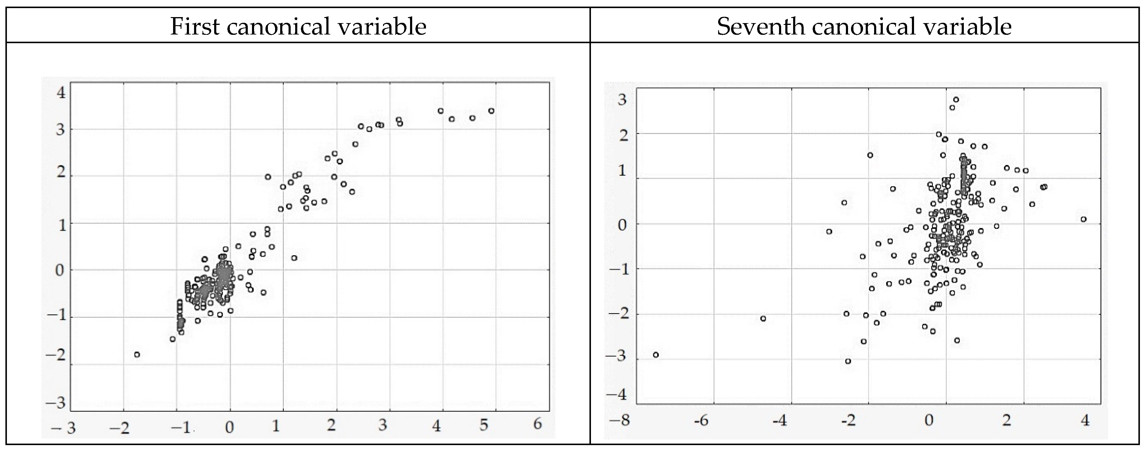
First canonical variable	0.3112	0.2749	0.0685	0.0605
Second canonical variable	0.1163	0.0812	0.0821	0.0573
Third canonical variable	0.1613	0.0890	0.0437	0.0241
Fourth canonical variable	0.0571	0.0252	0.0491	0.0216
Fifth canonical variable	0.0831	0.0319	0.0689	0.0265
Sixth canonical variable	0.0803	0.0227	0.0250	0.0071
Seventh canonical variable	0.0771	0.0182	0.0601	0.0142

Source: Own study based on [8].

). Factor loadings are interpreted as values of correlation between canonical and interchangeable variables in each analysed set. The greater they are (in terms of an absolute value), the more emphasis should be placed on this variable during the interpreting. T. Panek and J. Zwierzchowski [92] recommend interpreting variables for which the square of this correlation coefficient is greater than 0.50. In turn, G. Więcek and A. Sękowski [101] propose analysing only those variables for which the value of loads (not their squares) is greater than 0.30. For this analysis, it was assumed that the critical value of the correlation coefficient square is 0.20 (to facilitate the interpretation, those values were presented in Table 6 in bold and italics).

In the set of variables concerning the standard of living of the residents, for the first canonical root, the highest factor loading is presented by variable S27 (0.6762); for the second canonical variable, the highest factor load is shown by variable S10 (0.4852), for the third—variable S27 (0.3987), for the fourth—variable S11 (−0.3931), and the fifth—variable S17 (−0.3477). For the last two significantly static canonical roots, the greatest factor loadings were exhibited by variables S17 and S13 (-0.3031 and -0.3986, respectively). With regard to the set of variables concerning the renewable energy development level, for the first canonical variable, the highest factor loading is carried by variable R1 (0.7932), for the second—variable R5 (0.5088), for the third—variable R3 (−0.7187), for the fourth—variable R9 (0.3963), for the fifth—variable R1 (−0.5072), for the sixth and seventh—variable R9 (0.4900 and −0.5868, respectively).

In the literature on the topic, there are opinions, which claim that, in the interpretation of results obtained based on the canonical analysis, the interpretation of individual variables should be conducted using values of canonical factor loadings. This is substantiated by the fact that they are easy to understand intuitively. However, it is necessary to note that the values of such coefficients indicate correlations of individual input variables with canonical variables and, unlike the canonical weights, do not take into account the effects of covariance within a given set of input variables. As a result, the interpretation of canonical roots based on the values of correlation coefficients may lead to different conclusions than a more complete “multidimensional” interpretation based on canonical weights [93].

Based on the values of canonical weights and factor loadings, it can be concluded that the first statistically significant canonical root explained the following relationships:

• the higher the production of electricity and derived heat based on hydroenergy (R1), wind energy (R2) and renewable municipal waste (R5), the higher the average wage of workers (S11);
• the higher the production of electricity and derived heat based on hydroenergy (R1), wind energy (R2) and renewable municipal waste (R5), the lower the generation of hazardous waste (S28),
• as the share of renewable energy in final electricity consumption (R6) and the share of renewable energy in energy consumption in transport (R8) increase, so does the forestation rate. Therefore, it is possible to presume that activities related to the “greening” of the economy go hand in hand.

Based on the values of canonical weights and factor loadings for the second canonical root, it can be concluded that there is a positive correlation between the production of electricity and derived heat based on renewable municipal waste and the percentage of people with higher education in the age group 25–64 (S10). In turn, based on the fourth canonical root (or, more precisely, its weights and canonical loads), it can be concluded that the percentage of people at risk of poverty and social exclusion (S16) decreases as the production of electricity and derived heat based on hydroenergy (R1) increases. However, based on the values of canonical weights and factor loadings for the last necessary significant variable, it may be concluded that, as the installed heat pump capacity (R9) increases, the percentage of people with chronic diseases or health problems (S19) decreases.

When analysing factor loading values for the third, fourth and sixth canonical roots, it is possible to notice that in at least one analysed set, the square of the correlation coefficient between canonical variables and partial variables was less than 0.2 for all considered variables. For this reason, such canonical variables were not interpreted in terms of factor loadings and canonical weights.

In the subsequent step, the mean of the factor loading squares of every analysed set was determined for each statistically significant canonical variable, thus obtaining an indicator referred to as the extracted variance. In turn, by multiplying the said mean by the square of the canonical correlation, the redundancy value was obtained. The table below presents the values of the extracted (isolated) variance and redundancies (Table 7).

The most statistically significant canonical variable isolates more than 31% of the variance in the set of variables relating to the level of renewable energy development and nearly 7% in the second set (concerning the standard of living of EU residents). In turn, the second and third canonical variables isolate respectively 11.6% and 16% of the variance in the set describing RES, as well as 8% and 4% in the set of variables related to the standard of living. In the case of subsequent canonical variables, the degree of variance isolation in the set concerning the level of renewable energy development is significantly smaller; in the second set, the extracted (isolated) variance did not exceed 7%. The last statistically significant canonical variable isolates nearly 8% of the variance in the first set and 6% in the second set.

For the set of variables related to the standard of living of the EU residents, it is possible to explain 6.1%, 5.7%, 2.4%, 2.2%, 2.7%, 0.7%, and 1.4% of the variance of the set of variables describing the level of renewable energy development, respectively. In turn, with regard to the set of primary variables concerning the level of renewable energy development, it is possible to explain 27.5%, 8.1%, 8.9%, 2.5%, 3.2%, 2.3%, and 1.8% of the variance based on the first seven statistically significant canonical variables, respectively. Therefore, the fourth and subsequent statistically significant canonical variables already make a small specific contribution to explaining this variation. When comparing the amount of explained variance in both analysed sets of variables, it can be seen that in terms of each generated canonical root, the group of variables describing the level of RES development has a greater contribution to explaining the standard of living of the residents. This results in a research-relevant conclusion: variables describing the RES development level constitute a better predictor of variation in the standard of living that vice versa.

The next step involves the calculation of the total redundancy, interpreted as the average percentage of the variance explained in one set of variables for a second given set, based on all canonical variables. The conducted calculations show that the knowledge of values of variables describing the renewable energy development level allows explaining nearly 55.5% of the variance of variables from the set describing the standard of living of the EU residents. This value may be assessed as relatively high, and to obtain even better results, further research should be conducted in the future, using a different set of input variables and a changed number of such variables.

When studying multidimensional correlations between the standard of living and level of renewable energy development, it is worth noting the high and, more importantly, statistically significant (see Table 5) canonical correlation values. However, at this point, it should be emphasised that canonical correlation cannot be interpreted in the same manner as classical correlation (e.g., Pearson’s). These values are interpreted as correlations between the weighted sum values in each set and the weights calculated for subsequent canonical variables. The value of the greatest and most statistically significant canonical correlation was 0.94. For the last (seventh) statistically significant canonical variable, this value was nearly 0.49. The square of these canonical correlations constitutes a measure of the degree of explanation, through linear relationships, of the variability of one set of variables by the other input set, through successive pairs of canonical variables. For the first statistically significant canonical variable, the square of the canonical correlation is over 0.88, while for the second one, it is nearly 0.70. For the last statistically significant canonical variable (seventh), this coefficient is close to 0.24. It can be assumed that this generated model describes the analysed data sets relatively well.

The figure below presents the scatter plots of the first and last statistically significant canonical variable (Figure 2). The OX axis refers to the set of variables concerning the level of renewable energy development while the OY axis refers to the standard of living of the EU inhabitants.

For the first canonical variable, the scatter plot does not present any strong scatter of points representing the analysed objects. These points are arranged along a straight line. This indicates that the generated pairs of canonical variables carry a significant amount of information about the covariance of the two analysed sets of input variables. The proximity of most points (which in the case of canonical analysis represent the European Union regions) may indicate a similar structure of input variables. In the scatter plot compiled for the last statistically significant canonical variable, points representing the analysed objects are also arranged along an upwardly inclined line, yet are more scattered relative to the said line. This indicates that such a pair of canonical variables carries a significantly smaller amount of information about the covariance of two analysed variables than the first pair of canonical variables.

5. Conclusions

Initially, renewable energy was marginalised due to very high investment costs. However, their progressive decline indicates that renewable energy is currently perceived not only as a source of energy but also as an instrument that facilitates resolving many other global problems. Among other things, it is crucial for ensuring energy security, reducing the effects of environmental contamination and mitigating the influence of excessive greenhouse gas emissions, which is particularly important in the context of implementing the concept of sustainable development. One of the basic tasks of the state consists in ensuring energy security (especially important nowadays, from the perspective of the standard of living) which should not, however, take place at the cost of environmental degradation. Renewable energy sources generate zero to small amounts of pollution, which in the face of a deteriorating condition of the natural environment is an undeniable advantage.

The conducted studies aimed to detect correlations between the sets of variables describing the standard of living of the EU inhabitants and the level of renewable energy development. The canonical analysis appears to be the most appropriate statistical tool, which may be used to study multidimensional interactions between two sets of variables. Due to the multifaceted character of the analysed categories, the sole use of classical correlation analysis or multiple regression analysis seems to be inadequate. According to the author, for the analysis of socio-economic phenomena, it is important to popularise the use of multidimensional exploratory methods (such as canonical analysis) to identify correlations between compiled, multidimensional categories.

In the conducted studies, the canonical analysis was preceded by the creation of the author’s synthetic measures and the determination of the correlation coefficient between them. For the partial variables included in the study, the coefficient of variation for the constructed measure of the level of renewable energy development was over 47%, while the standard deviation was nearly 0.12 (with a mean value of nearly 0.25). This confirms the significant variation in the level of renewable energy development in the European Union. In turn, for the constructed synthetic measure of the standard of living, the classical variation coefficient was less than 10.5%, which indicates a relatively weak differentiation of the analysed phenomenon (for the analysed set of partial variables). In the case of three-quarters of the EU countries, the value of the synthetic measure did not exceed 0.49 (with a minimum value of 0.37 and a maximum value of 0.54). Based on the conducted correlation analysis, it can be concluded that there is a positive, moderate and statistically significant correlation between the standard of living of the EU residents and the level of renewable energy development (measured by synthetic measures constructed using the TOPSIS method) (Spearman’s rank correlation coefficient was nearly 0.47). Seven statistically significant canonical variables were identified using canonical analysis. Based on the value of the redundancy coefficient determined as part of the canonical analysis, it can be concluded that, with the knowledge of the considered variables describing the level of renewable energy development in the EU, it is possible to explain nearly 55.5% of the variance of variables from the set concerning the standard of living of the residents. In other words, more than half of the variation associated with the standard of living of the EU residents is determined by partial variables relating to the level of renewable energy development that were taken into account. It should also be mentioned that high values of canonical correlation coefficients were identified for statistically significant canonical variables. For the most statistically significant canonical variable, this coefficient was 0.94, while for the least statistically significant, it was 0.31.

The results of conducted studies (i.a. the ranking of countries in terms of the standard of living of the residents), can be used indirectly by, for example, central and self-government authorities responsible for local and regional development (including undertaking pro-social and pro-environmental actions) in the context of selecting the direction of socio-economic restructuring of individual countries and self-government units (taking into account the financial capacity of the society). Furthermore, the results of the studies may indirectly prompt self-government authorities to undertake actions directed towards more efficient use of the capacity for funding investment projects aimed to develop renewable energy technologies. Quantification of such important economic categories as the standard of living and the renewable energy sources development level in comparison with other areas may be conducive to initiating activities (e.g., of local authorities in shaping sustainable development strategies) directed towards stimulation of development aimed to achieve the highest standard of living while respecting natural resources. The conducted studies and obtained results may constitute the starting point for further analyses using different statistical methods (e.g., Granger causality analysis) and/or diagnostic variables, or to encourage similar studies at the level of other countries and self-government units. In further analyses, it would also be worth it to examine the spatial interactions between the phenomena analysed, including analysing autocorrelation and spatial heterogeneity, as well as constructing spatial regression models (including SEM and SLM models). It is possible to consider weighting the applied diagnostic variables based on expert opinions and/or statistical methods, which, however, in the case of spatial unit analyses, is a controversial solution.

References

- Bp p.l.c. Energy Outlook, 2020 Edition. Bp p.l.c. 2020. Available online: https://www.bp.com/content/dam/bp/business-sites/en/global/corporate/pdfs/energy-economics/energy-outlook/bp-energy-outlook-2020.pdf?utm_source=newsletter&utm_medium=email&utm_campaign=newsletter_axiosgenerate&stream=top (accessed on 2 March 2021).
- Fraunhofer ISE. Public Net Electricity Generation in Germany 2019: Share from Renewables Exceeds Fossil Fuels, FRAUNHOFER INSTITUTE FOR SOLAR ENERGY SYSTEMS ISE. 2020. Available online: https://www.ise.fraunhofer.de/content/dam/ise/en/documents/News/0120_e_ISE_News_Electricity%20Generation_2019.pdf (accessed on 28 March 2021).
- European Commission. Reflection Paper towards A Sustainable Europe by 2030; European Commission: Brussels, Belgium, 2019. [Google Scholar] [CrossRef]
- European Commission. Communication from the Commission to the European Parliament, the European Council, the Council, the European Economic and Social Committee and the Committee of the Regions the European Green Deal; European Commission: Brussels, Belgium, 2019. [Google Scholar]
- Njiru, C.W.; Letema, S.C. Energy Poverty and Its Implication on Standard of Living in Kirinyaga, Kenya. J. Energy 2018, 2018, 3196567. [Google Scholar] [CrossRef]
- Getie, E.M. Poverty of Energy and Its Impact on Living Standards in Ethiopia. J. Electr. Comput. Eng. 2020, 2020, 7502583. [Google Scholar] [CrossRef]
- Hussein, M.A.; Filho, W.L. Analysis of energy as a precondition for improvement of living conditions and poverty reduction in sub-Saharan Africa. Sci. Res. Essays 2012, 7, 2656–2666. [Google Scholar]
- Eurostat. Available online: https://ec.europa.eu/eurostat/web/main/data/database (accessed on 20 February 2021).
- Zeliaś, A. Poziom życia w Polsce i krajach Unii Europejskie; PWE: Warszawa, Poland, 2004. [Google Scholar]
- Luszniewicz, A. Statsytyka Społeczna: Podstawowe Problemy i Metody; PWE: Warszawa, Poland, 1982. [Google Scholar]
- Grzega, U. Poziom życia Ludności w Polsce—Determinanty i Zróżnicowania; Wydawnictwo Uniwersytetu Ekonomicznego w Katowicach: Katowice, Poland, 2012. [Google Scholar]
- Mourad, M.; Perez, A.; Richardson, C. Digital Inclusion Social Impact Evaluation; Final Report; One Global Economy: Washington DC, USA, 2014. [Google Scholar]
- Słaby, T. Poziom i jakość życia. In Statystyka Społeczna; Panek, T., Ed.; PWE: Warszawa, Poland, 2007; pp. 99–130. [Google Scholar]
- Chabior, A.; Fabiś, A.; Wawrzyniak, J.K. Starzenie się i Starość w Perspektywie Pracy Socjalnej; Centrum Rozwoju Zasobów Ludzkich: Warszawa, Poland, 2014. [Google Scholar]
- Frieske, K.W.; Popławski, P. Opieka i Kontrola; Interart: Warszawa, Poland, 1996. [Google Scholar]
- Tomaszewski, T. Aktywność człowieka. In Kształtowanie Motywacji i Postaw. Socjotechniczne Problemy Działalności Ideowo-Wychowawczej; Czapów, C., Ed.; Książka i Wiedza: Warszawa, Poland, 1976; pp. 88–89. [Google Scholar]
- Max-Neef, M.A. Human Scale Development. In Conception, Application and Further Reflections; The Apex Press: New York, NY, USA; London, UK, 1991. [Google Scholar]
- Murray, M.; Pauw, C.; Holm, D. The House as a Satisfier for Human Needs: A Framework for Analysis, Impact Measurement and Design. In Proceedings of the XXXIII IAHS World Congress on Housing Transforming Housing Environments through Design, Pretoria, South Africa, 27–30 September 2005; pp. 1–9. [Google Scholar]
- Ding, H.; Jiang, T.; Riloff, E. Why is an Event Affective? Classifying Affective Events based on Human Needs. In Proceedings of the Workshops at the Thirty-Second AAAI Conference on Artificial Intelligence, New Orleans, LA, USA, 2–7 February 2018; pp. 8–15. [Google Scholar]
- Słaby, T. Konsumpcja. Eseje Statystyczne; Difin: Warszawa, Poland, 2006. [Google Scholar]
- Sompolska-Rzechuła, A.; Oleńczuk-Paszel, A. Poziom życia ludności na obszarach wiejskich i miejskich w Polsce. Wieś Rol. 2017, 4, 77–96. [Google Scholar] [CrossRef]
- Piasny, J. Problem jakości życia ludności oraz źródła i mierniki ich określania. Ruch Prawniczy. Ekon. Socjol. 1993, 2, 73–92. [Google Scholar]
- Zeliaś, A. Dobór zmiennych diagnostycznych. In Taksonomiczna Analiza Przestrzennego Zróżnicowania Poziomu życia w Polsce W ujęciu Dynamicznym; Zeliaś, A., Ed.; Wydawnictwo Akademii Ekonomicznej w Krakowie: Kraków, Poland, 2000; pp. 35–55. [Google Scholar]
- Gotowska, M. Problemy definiowania poziomu i jakości życia. In Poziom i Jakość życia w Dobie Kryzysu; Gotowska, M., Wyszkowska, Z., Gotowska, M., Eds.; Wydawnictwo UTP: Bydgoszcz, Poland, 2013; pp. 11–24. [Google Scholar]
- Kryk, B. Jakość życia a społeczna odpowiedzialność przedsiębiorstwa za korzystanie ze środowiska. In Jakość życia w Perspektywie Nauk Humanistycznych, Ekonomicznych i Ekologii, Tomczyk-Tołkacz, J., Ed.; Akademia Ekonomiczna we Wrocławiu: Jelenia Góra, Poland, 2003; pp. 260–268. [Google Scholar]
- Sulich, A.; Grudziński, A.; Kulhánek, L. Zielony wzrost gospodarczy—Analiza porównawcza Czech i Polski. Pr. Nauk. Uniw. Ekon. Wrocławiu 2020, 64, 192–207. [Google Scholar] [CrossRef]
- Visser, W.; Pearce, D.; Markandya, A.; Barbier, E.B. Blueprint for a Green Economy; Greenleaf Publishing Limited: South Yorkshire, UK, 2013; pp. 70–76. [Google Scholar]
- UNEP. Towards a Green Economy: Pathways to Sustainable Development and Poverty Eradication—A Synthesis for Policy Makers; United Nations Environment Programme: Saint-Martin-Bellevue, France, 2011. [Google Scholar]
- Krakowińska, E. “Zielone” miejsca pracy w energetyce odnawialnej w Polsce i na Mazowszu. In Rola Odnawialnych źródeł Energii w Rozwoju Społeczno-Ekonomicznym Kraju i Regionu; Nowak, A.Z., Ed.; Wydawnictwo Naukowe Wydziału Zarządzania Uniwersytetu Warszawskiego: Warszawa, Poland, 2016; pp. 69–96. [Google Scholar]
- Maśloch, G. Construction Autonomous Energy Regions in Poland—Utopia or Necessity? Stud. Prawno-Ekon. 2018, 106, 251–264. [Google Scholar] [CrossRef]
- Nowak, A.Z.; Zaborowska, W. Wprowadzenie. In Rola Odnawialnych źródeł Energii w Rozwoju Społeczno-Ekonomicznym Kraju i Regionu; Nowak, A.Z., Ed.; Wydawnictwo Naukowe Wydziału Zarządzania Uniwersytetu Warszawskiego: Warszawa, Poland, 2016; pp. 10–13. [Google Scholar]
- Kochańska, E. Determinanty Rozwoju Odnawialnych źródeł Energii; Centrum Badań i Innowacji Pro-Akademia: Łódź, Poland, 2014. [Google Scholar]
- WWF. Demaskowanie Mitów: Obalanie Mitów o Energii Odnawialnej; WWF International: Gland, Switzerland; Warsaw, Poland, 2014. [Google Scholar]
- Gnutek, Z. Wybrane aspekty użytkowania energii w rolnictwie. Inżynieria Rol. 2011, 9, 49–56. [Google Scholar]
- Graczyk, A.M. Koordynacja polityki energetycznej—Regionalne ujęcie wsparcia odnawialnych źródeł energii w świetle Strategii rozwoju energetyki na Dolnym Śląsku. Barom. Reg. 2016, 14, 113–120. [Google Scholar]
- McLuhan, M.; Nevitt, B. Take Today—The Executive as Dropout; Harcourt Brace Jovanovich: San Diego, CA, USA, 1972. [Google Scholar]
- Zalega, T. Wykorzystanie Odnawialnych źródeł Energii w Gospodarstwach Domowych seniorów w Polsce w świetle wyników badań własnych. In Rola Odnawialnych źródeł Energii w Rozwoju Społeczno-Ekonomicznym Kraju i Region; Nowak, A.Z., Ed.; Wydawnictwo Naukowe Wydziału Zarządzania Uniwersytetu Warszawskiego: Warszawa, Poland, 2016; pp. 48–68. [Google Scholar]
- Borys, G. System wsparcia energetyki prosumenckiej w Polsce. Studia Ekonomiczne. Zesz. Nauk. Uniw. Ekon. Katowicach 2014, 198, 35–43. [Google Scholar]
- Woźniak, M.; Saj, B. Odnawialne źródła energii w badaniach ankietowych mieszkańców województwa podkarpackiego. Zesz. Nauk. Inst. Gospod. Surowcami Miner. Energią PAN 2018, 61–80. [Google Scholar] [CrossRef]
- Creţan, R.; Vesalon, L. The Political Economy of Hydropower in the Communist Space: Iron Gates Revisited. Tijdschr. Econ. Soc. Geogr. 2017, 108, 688–701. [Google Scholar] [CrossRef]
- Vãran, C.; Creţan, R. Place and the spatial politics of intergenerational remembrance of the Iron Gates displacements in Romania, 1966–1972. Area 2018, 50, 509–519. [Google Scholar] [CrossRef]
- Świątek, M.; Cedro, A. Odnawialne źródła Energii w Polsce ze Szczególnym Uwzględnieniem Województwa Zachodniopomorskiego; Uniwersytet Szczeciński: Szczecin, Poland, 2017. [Google Scholar]
- European Commission. Communication from the Commission. A Clean Planet for All. A European Strategic Long-Term Vision for a Prosperous, Modern, Competitive and Climate Neutral Economy; COM(2018) 773 Final; European Commission: Brussels, Belgium, 2018. [Google Scholar]
- Jędrak, J.; Konduracka, E.; Badyda, A.J.; Dąbrowiecki, P. Wpływ Zanieczyszczeń Powietrza na Zdrowie [Impact of Air Pollution on Health]; Krakowski Alarm Smogowy: Kraków, Poland, 2017. [Google Scholar]
- Szyszkowicz, M.; Willey, J.B.; Grafstein, E.; Rowe, B.H.; Colman, I. Air Pollution and Emergency Department Visits for Suicide Attempts in Vancouver, Canada. Environ. Health Insights 2010, 4, EHI.S5662. [Google Scholar] [CrossRef] [PubMed]
- Rzędowska, A.; Rzędowski, J. Smog. Czas na Decydujące Starcie. Raport; Instytut Jagielloński: Warszawa, Poland, 2018. [Google Scholar]
- WHO Regional Office for Europe—OECD. Economic Cost of the Health Impact of Air Pollution in Europe: Clean Air, Health and Wealth; WHO Regional Office for Europe: Copenhagen, Denmark, 2015. [Google Scholar]
- Tomala, M. Energia odnawialna jako kluczowy element bezpieczeństwa zaopatrzenia energetycznego i środowiskowego państw nordyckich, Bezpieczeństwo. Teor. Prakt. 2016, 1, 105–117. [Google Scholar]
- Ignarska, M. Odnawialne źródła energii w Polsce. Poliarchia 2013, 1, 57–72. [Google Scholar] [CrossRef]
- Skubiak, B. Rola Samorządów w Przezwyciężaniu Barier Rozwoju Odnawialnych źródeł Energii. In Trendy i Wyzwania ZrównOważonego Rozwoju; Kryk, B., Ed.; Uniwersytet Szczeciński: Szczecin, Poland, 2011; pp. 275–294. [Google Scholar]
- Ligus, M.; Poskrobko, T.; Sidorczuk-Pietraszko, E. Pozaśrodowiskowe Efekty Zewnętrzne w Lokalnych Systemach Energetycznych; Fundacja Ekonomistów Środowiska i Zasobów Naturalnych: Białystok, Poland, 2015. [Google Scholar]
- REN21. Renewables 2020 Global Status Report; REN21 Secretariat: Paris, France, 2020. [Google Scholar]
- BP p.l.c. BP Statistical Review of World Energy 2020, 69th ed.; Statistical Review of World Energy: London, UK, 2020. [Google Scholar]
- IRENA. Renewable Capacity Statistics 2019; International Renewable Energy Agency (IRENA): Abu Dhabi, United Arab Emirates, 2019.
- Simionescu, M.; Bilan, Y.; Krajňáková, E.; Streimikiene, D.; Gędek, S. Renewable Energy in the Electricity Sector and GDP per Capita in the European Union. Energies 2019, 12, 2520. [Google Scholar] [CrossRef]
- Grabara, J.; Tleppayev, A.; Dabylova, M.; Mihardjo, L.W.W.; Dacko-Pikiewicz, Z. Empirical Research on the Relationship Amongst Renewable Energy Consumption, Economic Growth and Foreign Direct Investment in Kazakhstan and Uzbekistan. Energies 2021, 14, 332. [Google Scholar] [CrossRef]
- Llamosas, C.; Sovacool, B.K. The future of hydropower? A systematic review of the drivers, benefits and governance dynamics of transboundary dams. Renew. Sustain. Energy Rev. 2021, 137, 110495. [Google Scholar] [CrossRef]
- Walesiak, M. Uogólniona Miara Odległości GDM w Statystycznej Analizie Wielowymiarowej z Wykorzystaniem Programu R; Wydawnictwo Uniwersytetu Ekonomicznego we Wrocławiu: Wrocław, Poland, 2011. [Google Scholar]
- Redclif, M. Critical Concepts in the Social Sciences; Routledge Taylor & Francis: London, UK; New York, NY, USA, 2005. [Google Scholar]
- Bleys, B. Alternative Welfare Measures. MOSI Work. Pap. 2005, 12, 1–15. [Google Scholar]
- Lawn, P.A. A theoretical foundation to support the Index of Sustainable Economic Welfare (ISEW), Genuine Progress Indicator (GPI), and other related indexes. Ecol. Econ. 2003, 44, 105–118. [Google Scholar] [CrossRef]
- Gasparatos, A.; El-Haram, M.; Horner, M. A critical review of reductionist approaches for assessing the progress towards sustainability. Environ. Impact Assess. Rev. 2008, 28, 286–311. [Google Scholar] [CrossRef]
- UNDP. Human Development Indices and Indicators 2018 Statistical Update; United Nations Development Programme: Washington, DC, USA, 2018. [Google Scholar]
- UNDP. Human Development Report 2015. Work for Human Development—TECHNICAL NOTES. 2015, pp. 1–10. Available online: http://hdr.undp.org/sites/default/files/hdr2015_technical_notes.pdf (accessed on 6 March 2021).
- The Economist Intelligence Unit’s Quality-of-Life Index. 2005. Available online: https://www.economist.com/media/pdf/quality_of_life.pdf (accessed on 6 March 2021).
- OECD. Better Life Index: Definitions and Metadata. 2019. Available online: https://www.oecd.org/statistics/OECD-Better-Life-Index-definitions-2019.pdf (accessed on 6 March 2021).
- NEF. Happy Planet Index 2016 Methods Paper. Available online: https://static1.squarespace.com/static/5735c421e321402778ee0ce9/t/578cc52b2994ca114a67d81c/1468843308642/Methods+paper_2016.pdf (accessed on 28 March 2021).
- Green, M.; Harmacek, J.; Krylova, P. 2020 Social Progress Index; Executive Summary; Social Progress Imperative: Washington, DC, USA, 2020; Available online: https://www.socialprogress.org/static/37348b3ecb088518a945fa4c83d9b9f4/2020-social-progress-index-executive-summary.pdf (accessed on 28 March 2021).
- Almond, R.E.A.; Grooten, M.; Petersen, T. Living Planet Report—2020: Ratunek dla Różnorodności Biologicznej; WWF: Gland, Switzerland, 2020. [Google Scholar]
- Lazarus, E.; Zokai, G.; Borucke, M.; Panda, D.; Iha, K.; Morales, J.C.; Wackernagel, M.; Galli, A.; Gupta, N. Working Guidebook to the National Footprint Accounts; Global Footprint Network: Oakland, CA, USA, 2014. [Google Scholar]
- The Global Green Economy Index. Available online: https://dualcitizeninc.com/global-green-economy-index/ (accessed on 28 March 2021).
- Karpińska-Mizielińska, W. Instytucje Infrastruktury Rynkowej w Kreowaniu Przedsiębiorczości Lokalnej; Fundacja Promocji Rozwoju im. E. Lipińskiego: Warszawa, Poland, 1999. [Google Scholar]
- Nermend, K. Metody Analizy Wielokryterialnej i Wielowymiarowej We Wspomaganiu Decyzji; PWN: Warszawa, Poland, 2017. [Google Scholar]
- Kuc, M. Konwergencja społeczna i ekonomiczna regionów państw nordyckich. Coll. Econ. Anal. Ann. 2016, 41, 175–188. [Google Scholar]
- Malinowski, M.; Smoluk-Sikorska, J. Spatial Relations between the Standards of Living and the Financial Capacity of Polish District-Level Local Government. Sustainability 2020, 12, 1825. [Google Scholar] [CrossRef]
- Wysocki, F. Metody Taksonomiczne w Rozpoznawaniu Typów Ekonomicznych Rolnictwa i Obszarów Wiejskich; Wydawnictwo Uniwerystetu Przyrodncizego w Poznaniu: Poznań, Poland, 2010. [Google Scholar]
- Młodak, A. Analiza Taksonomiczna w Statystyce Regionalnej; Difin: Warszawa, Poland, 2006. [Google Scholar]
- Hwang, C.L.; Yoon, K. Multiple Attribute Decision Making: Methods and Applications; Springer: New York, NY, USA, 1981. [Google Scholar]
- Korol, J.; Szczuciński, P. Ekonometryczne Modelowanie Procesów Gospodarki Regionalnej Opartej na Wiedzy; Wydawnictwo Adam Marszałek: Toruń, Poland, 2009. [Google Scholar]
- Kaufman, L.; Rousseeuw, P.J. Finding Groups in Data: An Introduction to Cluster Analysis; John Wiley & Sons Inc.: Hoboken, NJ, USA, 2005. [Google Scholar]
- UNESCO. IDAMS. Internationally Developed Data Analysis and Management Software Package; UNESCO: Paris, France, 2008. [Google Scholar]
- Ter Braak, C.J.F. Interpreting canonical correlation analysis through biplots of structure correlations and weights. Psychometrika 1990, 55, 519–531. [Google Scholar] [CrossRef]
- Cavadias, G.S.; Ouarda, T.B.M.J.; Bobée, B.; Girard, C. A canonical correlation approach to the determination of homogeneous regions for regional flood estimation of ungauged basins. Hydrol. Sci. J. 2001, 46, 499–512. [Google Scholar] [CrossRef]
- Hardoon, D.R.; Szedmak, S.; Shawe-Taylor, J. Canonical Correlation Analysis. In An Overview with Application to Learning Methods; University of London: London, UK, 2003. [Google Scholar]
- Weenink, D. Canonical Correlation Analysis. IFA Proc. 2003, 25, 81–99. [Google Scholar]
- Naylor, M.G.; Lin, X.; Weiss, S.T.; Raby, B.A.; Lange, C. Using Canonical Correlation Analysis to Discover Genetic Regulatory Variants. PLoS ONE 2010, 5, e10395. [Google Scholar] [CrossRef]
- Krzyśko, M.; Łukaszonek, W.; Wołyński, W. Canonical Correlation Analysis in the Case of Multivariate Repeated Measures Data. Stat. Transit. New Ser. 2018, 19, 75–85. [Google Scholar] [CrossRef][Green Version]
- Ebenezer, O.R. Canonical Correlation Analysis of Poverty and Literacy Levels in Ekiti State, NIGERIA. Math. Theory Model. 2012, 2, 31–39. [Google Scholar]
- Chin-Tsai, K. Life Quality and Job Satisfaction: A Case Study on Job Satisfaction of Bike Participants in Chiayi County Area. J. Int. Manag. Stud. 2011, 6, 1–9. [Google Scholar]
- Saeed, T.; Tularam, G.A. Relations between fossil fuel returns and climate change variables using canonical correlation analysis. Energy Sources Part B Econ. Plan. Policy 2017, 12, 675–684. [Google Scholar] [CrossRef]
- Santos-Alamillos, F.J.; Pozo-Vázquez, D.; Ruiz-Arias, J.A.; Lara-Fanego, V.; Tovar-Pescador, J. Analysis of Spatiotemporal Balancing between Wind and Solar Energy Resources in the Southern Iberian Peninsula. J. Appl. Meteorol. Clim. 2012, 51, 2005–2024. [Google Scholar] [CrossRef]
- Panek, T.; Zwierzchowski, J. Statystyczne Metody Wielowymiarowej Analizy Porównawczej: Teoria i Zastosowania; Oficyna Wydawnicza SGH: Warszawa, Poland, 2013. [Google Scholar]
- Jaba, E. The “3 sigma” rule used for the identification of the regional disparities. Yearbook of the “Gheorghe Zane”. Inst. Econ. Res. 2007, 16, 47–57. [Google Scholar]
- Kasunic, M.; McCurley, J.; Goldenson, D.; Zubrow, D. An Investigation of Techniques for Detecting Data Anomalies in Earned Value Management Data; Software Engineering Institute: Pittsburgh, PA, USA, 2011. [Google Scholar]
- Noble, R.B., Jr. Multivariate Applications of Bayesian Model Averaging; Virginia Polytechnic Institute: Blacksburg, VA, USA, 2000. [Google Scholar]
- Tadeusiewicz, R.; Izworski, A.; Majewski, J. Biometria; AGH: Kraków, Poland, 1993. [Google Scholar]
- Thompson, B. Fundamentals of Canonical Correlation Analysis: Basics and Three Common Fallacies in Interpretation; University of New Orleans and Louisiana State University Medical Center: New Orleans, LA, USA, 1987. [Google Scholar]
- World Economic Forum. Fostering Effective Energy Transition, 2020 ed.; WWF: Cologny, Germany; Geneva, Switzerland, 2020. [Google Scholar]
- GUS. Energia ze źródeł Odnawialnych w 2019 r; Główny Urząd Statystyczny: Warszawa, Poland, 2020.
- Kopczewska, K.; Kopczewski, T.; Wójcik, P. Metody Ilościowe w R. Aplikacje Ekonomiczne i Finansowe; CeDeWu: Warszawa, Poland, 2009. [Google Scholar]
- Więcek, G.; Sękowski, A. Powodzenie w kształceniu integracyjnym a wybrane zmienne psychospołeczne—Weryfikacja modelu teoretycznego. Rocz. Psychol. 2007, 10, 89–111. [Google Scholar]