1. Introduction
Solar and wind energy are slowly becoming significant players in the Polish energy system. This is particularly visible from a perspective of their rated capacity, which, as of the end of 2020, was 3420 MW [
1] and 6347 MW [
2], respectively, for solar and wind. Although such capacities correspond to 19.8% of the total installed capacity [
3], the share of solar and wind energy in satisfying the national electrical energy demand remains relatively low, at 1.4% and 9.2%, respectively. (Estimation based on Entso data on wind generation in Poland [
4], which in 2020 was 15.2 TWh; electricity demand in Poland, which was 165.5 TWh [
5]; and assuming photovoltaic (PV) generation as 1 MWh per 1 kW of installed capacity. For PV, assumption was made that, over the year 2020, generation was calculated for mean installed capacity of that at the beginning of 2020 (1300 MW) and end of 2020 (3420 MW), namely 2360 MW).
With a growing share of solar and wind sources, their efficient integration to the existing structure of the power system becomes a major challenge [
6]. The complexity of the problem lies in an intrinsically variable and nondispatchable nature of solar and wind generators but also in limited flexibility of the available infrastructure.
In power systems with a nonexistent or low share of variable generators, the unpredictability was historically concerning, mostly on the demand side. In the past, many research works have been dedicated to the problem of developing precise day-ahead energy demand forecasting tools, applying methods, such as Artificial Neural Networks combined with wavelet transformation [
7], Deep Neural Networks [
8] or various data-driven approaches, as presented in a review by Liu et al. [
9]. On the other hand, the supply side was considered as fully controllable with a safety margin reserved for unexpected individual units failures or sudden spikes in power demand. With the advent of large-scale solar and wind power generators (in particular, from the perspective of their high installed capacities in relation to the load but still relatively small share in satisfying the demand), the problem of energy supply forecasting became a pressing need to efficiently operate the power system. Precise forecasts are mandatory not only for a transmission system operator but also for owners of variable power stations who want to actively participate in energy markets. Furthermore, as stated by Jacobson and Deluchi [
10], forecasting power generation from variable renewable generators is essential from the perspective of their efficient integration to the grid.
The main contribution of this paper is presenting a model for a day-ahead wind power prediction for the whole country in the example, Poland, not by applying models to individual wind farms but for the whole country at once.
The two following subsections will present a nonexhaustive literature review summarizing most recent works in the area of wind power forecasting. The first subsection will analyse articles discussing wind power forecasting outside Poland and the second one those focusing on Poland, as they can be directly used later on in the results discussion section.
Section 2 describes machine learning methods, a training strategy, details of numerical weather prediction (NWP) forecasting and wind power generation data.
Section 3 describes results of the study, including analysis of special cases.
Section 4 discusses the results, and
Section 5 concludes the paper.
1.1. Wind Power Forecasting
Over the recent years, several review articles have been published that analysed, in detail, various wind power forecasting methods and approaches. A review by Hanifi et al. [
11] provided a critical overview on physical, statistical and hybrid approaches to wind power forecasting. Their review not only indicated the past and current trends in this area of research but also highlighted future research directions, which include a need to develop more advanced and cost-effective forecasting methods; improve data processing and error post-processing, due to a proliferating amount of available data; and creating specific models for an off-shore wind power prediction, as such wind turbines operate in different weather conditions. Importantly, the authors noted that there is a lack of consensus with regard to the standard baseline model, which could be used as a reference for the newly developed ones. Furthermore, the review work by Hanifi et al. analysed the structure of input variables used in wind power prediction models. Their findings indicate that, among 40 analysed articles, exactly 50% used wind speed, followed by 25% that has also included air temperature. Very few studies used predictors, such as “generation hour” or “turbulence intensity”. The findings presented by Hanifi et al. are in line with the results presented by Lin and Liu [
12], who also found that wind speed, wind direction, temperature and humidity are the most commonly used wind power predictors. According to Hanifi et al., the most commonly used metrics for model evaluation are root mean square error (RMSE), normalized RMSE (nRMSE), mean absolute error (MAE) and mean absolute percentage error (MAPE). Another review work by Santhos et al. [
13] discussed differences between wind speed and wind power forecasting. In their work, they have also provided a temporal (time horizon) classification of forecasting models. According to it, one can distinguish very short-term forecasting (from a few seconds to 30 min), short-term forecasting (from 30 min to day-ahead), medium-term forecasting (from day-ahead to month-ahead) and long-term forecasting (more than month-ahead). Santhos et al. summarize the potential of hybrid method approach, which can yield an increase in forecast accuracy.
A study by Zhang et al. [
14] discussed the development of probabilistic wind power forecasting methods. Such an approach is suggested by the authors, since wind-to-power conversion is a complex and nonlinear problem. By using the probabilistic approach, one can not only obtain the forecast but also the quantitative information on the uncertainty. Considering above, Zhang et al. have distinguished the following three main categories of wind power forecast incorporating the uncertainty: probabilistic forecasting, risk index forecasting and scenario forecasting. Another work by Yan et al. [
15] conducted yet another in-depth review on the wind power probabilistic forecasting, with a special attention paid to the uncertainty factors, modelling approaches and time horizons. The authors state that the probabilistic wind speed forecasting brings additional benefits by reducing the risk of a deterministic prediction, improves the process of power system scheduling, reduces operating costs of wind farms and the power system and improves a wind power grid integration.
The day-ahead wind power forecasting problem was widely discussed by Yang et al. [
16], whereas the improved clustering algorithm was proposed and Zheng et al. [
17], where a two-stage hybrid model approach was proposed. High resolution NWP models, downscaled with a computational fluid model, were proposed by Mana et al. [
18], with a finding that they can perform as good or better than statistical methods. A novel variational model decomposition and long, short-term memory were introduced by Shi et al. [
19]. There was an interesting finding that some methods perform better at the beginning of the day and others at the end of the day.
A review article by Augustyn and Kamińska [
20] provides a good overview of most commonly applied forecasting methods. The following classification can be applied:
persistence models—which assume that wind power at time t is the same as in t—Δt;
physical models—which use a combination of wind turbine/characteristic power curve and numerical weather prediction (NWP) model data to generate forecasts;
statistical models—include time series and machine learning models. The time series-based models are autoregressive approach, autoregressive moving average and autoregressive integrated moving average. Models with exogenous inputs are also applied. Recently, models based on Artificial Neural Networks (ANN) gained popularity. They are often combined with other approaches, such as wavelet transformation, k-nearest neighbour algorithms and evolutionary optimization techniques. Techniques mentioned earlier can be naturally used independently.
hybrid methods—is an approach when both large amounts of historical data and physical models are applied. Hybrid method aims at using the strengths of both approaches.
Summarizing the above, the research in the field of wind power forecasting is focused on precise weather predictions on different timescales and postprocessing them to energy with physical, statistical and hybrid models.
1.2. Wind Power Forecasting in Poland
This section presents an overview of recent articles dedicated to wind power forecasting in the context of the Polish power system.
An article by Rubanowicz [
21] analysed several statistical methods for generating short-range wind power forecasts from a wind farm. The results of his investigation have revealed that Holt method outperformed the remaining approaches, in terms of forecast’s accuracy. Popławski et al. [
22] presented a one-day-ahead energy production model for a wind farm with 15 wind turbines. Their model included Unified Model forecasts from the Interdisciplinary Centre for Mathematical and Computational Modelling. Considering the MAPE criterion, their model was characterized with 46.9% error. Karkoszka [
23] presented an overview of various methods (physical, statistical and hybrid) to forecast wind power generation from wind farms. As input data, various NWP models have been considered.
Baczyński and Piotrowski [
24] analysed a day-ahead wind energy production forecast model based on ANN. Their analysis revealed that wind speed is a crucial input parameter in determining the model’s accuracy. Best results have been obtained by combining several neural networks. In another work, Popławski and Szeląg [
25] have analysed the possibility of using Hurst exponent to predict the instability of wind power generation. Their findings indicate that this approach can decrease the normalized MAPE (nMAPE) by 0.64%. Szeląg [
26] used wind speed, temperature and air pressure as input variables to predict a power output from a wind farm consisting of 10 turbines, each with a nominal capacity of 2.5 MW. The forecasting model was able to predict the energy generation, with nMAPE equal to 6.63%. However, the author did not use real meteorological forecasts. Instead, random error to measurements had been introduced. Hossa et al. [
27] used wind speed measurements to predict wind power generation from a fleet of 19 wind turbines. A multilevel regression method was applied and yielded a mean error equal to 12%.
Rubanowicz [
28] applied an Elman ANN to recreate the power generation from the selected wind farm. The results of his analysis highlight the importance of including the wind speed and wind direction as input variables. Rubanowicz stresses a need for careful evaluation of input data, since measuring errors often lead to skewed forecasts, as the model has been created based on an invalid training subset. A study by Malska and Mazur [
29] has shown that wind speed variability on a spatial scale can lead to different power outputs of wind turbines, even if these are located close to each other, indicating, thereby, a need for downscaling and more detailed measurements. A work by Baczyński and Kopyt [
30] considered two wind farms located in Poland. For them, they have created wind power forecasts for the next 48 h based on wind speed forecasts available from NWP. The conversion of wind speed to wind power, based on ANN, had been applied. The best results had been obtained by combining two NWP models.
Czapaj et al. [
31] discussed various forecasting methods (persistent, regressions, exponential smoothing) for demand and supply forecasting in energy clusters to find that only multivariate adaptive regression splines yield satisfactory results. Poławski and Szeląg [
32] used fractal theory to generate short-term wind power forecasts. Pietrzak and Świderski [
33] proposed a relevant extension to the existing database of wind speed measurements. Namely, they paid attention to the fact that wind speed measurements can not only be obtained from the meteorological institute but are also commonly generated by institutions managing transmission networks or roads. Greater spatial coverage of wind speed measurements could improve the quality of forecasting models.
Summarizing the above, the research in Poland is mainly focused on using observational data to analyse the possibility of predicting energy production, if precise forecast will be provided. Only local implementations are examined with short range prediction for a few wind turbines. In terms of methods, statistical ones are usually used, with most research focused on ANN implementations. Up to now, there is no research on the subject of day-ahead wind power forecasting for the whole country in Poland.
1.3. Research Questions
Considering the literature review presented in
Section 1.1 and
Section 1.2, as well as the general context and the increasing role of wind power in the Polish energy system, the objectives of this work are summarized as follows:
Is it possible to predict day-ahead wind power generation in Poland with high accuracy?
Which machine learning methods predict day-ahead wind power generation with the smallest error?
Is there seasonal or daily variation of model errors?
What are characteristic weather conditions for forecasts with small and big errors?
2. Materials and Methods
To simulate energy generation from wind turbines installed in Poland, four machine learning methods were used, with wind speed forecast from NWP model, energy generation time series (available online
https://www.pse.pl) and localization of wind turbines in Poland (available online
https://www.ure.gov.pl) used as input data.
The input data was divided into training, validation and testing subsets. Data from 2018–2019 was divided into training and validation subsets (70–30), whereas year 2020 was used for testing. The same subsets were considered in all models. All error metrics in this article are calculated for data from 2020.
Computation of MAPE and RMSE is a common way to measure and assess the error of a model in predicting quantitative data. Formally, it is defined as follows, Equations (1) and (2), respectively:
where
n stands for number of elements,
xi stands for observed value and
yi stands for predicted value.
Both Equations (1) and (2) deal directly with the residuals produced by considered models. The decision whether a model performs well is made by the assessment of the magnitude metric. Small error values point to an acceptable predictive ability, while large values suggest otherwise. Analysing error metrics is crucial to consider the nature of the data set, because outliers could impact on the total error metric. For that reason, it is important to compute and assess more than one metric. Wide comparison of the performance evaluation metrics of wind generation prediction models, ANN solutions and time series analysis that can be used was given by Hanifi et al. [
9]. RMSE and MAPE metrics were pointed to as one of the most frequently applicable, with the RMSE highly considered.
2.1. Machine Learning Methods
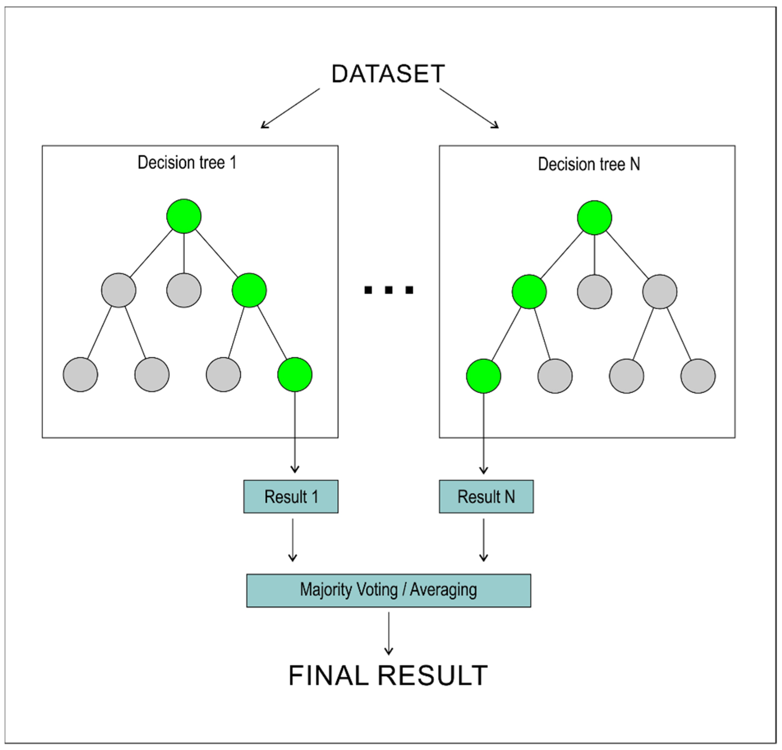
The Random Forest (RF), first proposed by Breiman [
34], is an ensemble learning, decision-tree-based method constructed by creating a series of decision trees from bootstrapped training samples. Computations were done with the Random Forest R package [
35], with default values of tuneable parameters. Schematic diagram of the Random Forest method is presented in
Figure 1.
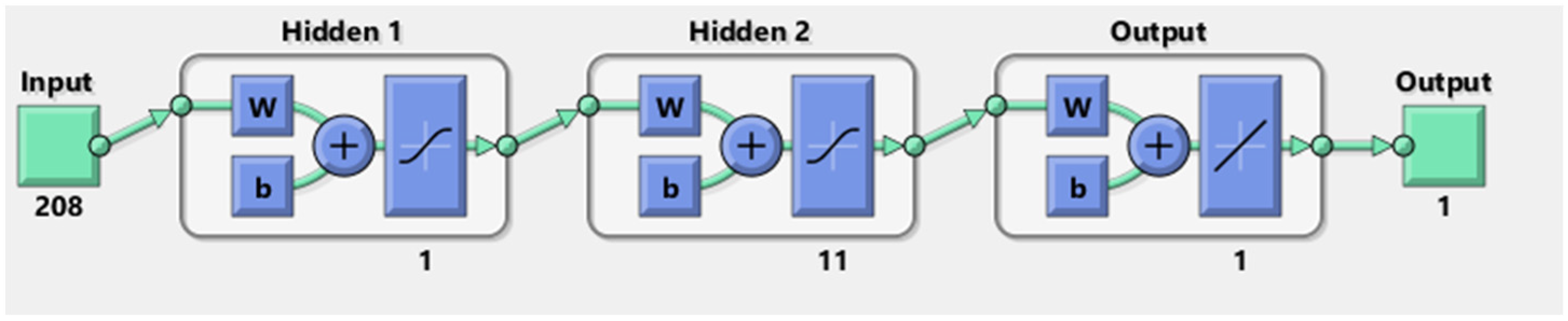
The Artificial Neural Network (ANN) model was created in Matlab R200b. A multilayer perceptron ANN was considered for further analysis. In a typical ANN, three layers can be distinguished: input layer (exogenous variables), hidden layer (nonlinear transformation of inputs to outputs) and output layer (endogenous variables). The number of neurons in the hidden layer is decided empirically by testing various configurations. The number of hidden layers is usually one or two, as these two options can cover the majority of fitting problems. In total, we tested ANN with 1 and 2 hidden layers, each having from 1 to 20 hidden neurons. Sigmoid and linear activation functions were used, respectively, in hidden and output layers. Prior to ANN creation, the data was normalized. The Levenberg–Marquardt backpropagation algorithm was selected to train the neural network and update the weights and biases. In total, 420 different ANN architectures were analysed, and the one best performing, in terms of mean absolute percentage error, was selected. The schematic diagram of ANN method is presented in
Figure 2.
A Deep Neural Network (DNN) is principally a classic ANN with more than one hidden layer. The method is said to be particularly beneficial when dealing with large datasets, for example, in recognition of speech or image [
36]. In this article, an implementation of deep learning from the H2O data science platform was used [
37]. Its structure is based on a feedforward multilayer network. Learning procedure concerns adaptation of neuron weights in order to minimize training error through a backpropagation algorithm. The information between layers is transmitted with a modification made by a nonlinear activation function. Multiple levels of nonlinearity lead to better feature extraction and information gain. There is a considerable number of parameters that affect DNN performance, such as number of layers, number of neutrons in each layer, type of activation function and number of training iterations (epochs). Based on a manual tuning, an optimal net’s architecture was found to have 3 hidden layers, each with 200 neurons. The number of epochs was boosted to 300.
Extreme Gradient Boosting (XGB) is one of the most efficient and popular implementations of gradient boosting algorithms and was proposed by Chen and Guestrin [
38] as R package xgboost. It develops an ensemble of decision trees in a sequential way. Unlike in RF, each tree is a weak learner—it merely outperforms a random guess [
39]. At each iteration, a new tree is grown, based on information from a previous model. The information concerns pieces of training data where the model had the largest error, which is foundational for minimizing a loss function. The process is a sort of gradient descent algorithm. Every tree added to the model slightly improves its performance. This novel algorithm structure results in substantial scalability of XGBoost and computational time about 10 times faster than other methods. The method offers several tuning hyperparameters, which control, e.g., a number of trees (nrounds), their maximum depth (max_depth) and learning rate (eta). Considering our dataset, the parameters were manually optimized as follows: nrounds was enlarged to 10,000, with a threshold of early stopping set to 5, eta was decreased to 0.2, and max depth was set to 6.
2.2. ALARO Model
On 27 November 2020, the creation of the new consortium “A Consortium for COnvection-scale modeling Research and Development” (ACCORD), was approved for the community development of numerical models of limited area at convective scale. The creation of this consortium results from the culmination of a merging process between the consortia Aire Limitée Adaptation Dynamique Développement International (ALADIN), Regional Cooperation for Limited Area modelling in Central Europe (RC-LACE) and High-Resolution Limited Area Model (HIRLAM), for the development of state-of-art atmospheric limited area numerical models, with application to operations.
The ACCORD system (previously ALADIN system) is an NWP system developed by the international ACCORD consortium for operational weather forecasting and research purposes. The ALADIN NWP system is based on a code that is shared with the Integrated Forecast System (IFS) global model developed by the European Centre for Medium-Range Weather Forecasts (ECMWF) and the Action de Recherche Petite Echelle Grande Echelle (ARPEGE) global NWP model used for operational weather forecasting at Météo-France [
40].
One of the consortium’s development work is to provide several configurations of limited-area model (LAM), which were precisely validated to be used for operational weather forecasting at the 16 partner institutes. These configurations are called the ALADIN canonical model configurations (CMCs). Currently, there are three canonical model configurations: 1. ALADIN baseline CMC, 2. Application of Research to Operations at Mesoscale (AROME) CMC and 3. ALADIN–AROME (ALARO) CMC. AROME CMC and ALARO CMC are operationally used in IMWM–NRI, together with the CY43T2 [
41].
The background model data come from operational forecast results of nonhydrostatic ALARO CMC model. Operational model ALARO CMC has a horizontal resolution of 4 km × 4 km and 70 vertical levels, and the forecast length is 72 h. The size of ALARO CMC domain is 799 × 799 points, centred on the geographical point 17.5° E 52.5° N. The location of the lowest model level is at 9 m above ground level, and the model top is located at 65 km above ground level. Lateral and boundary conditions for the ALARO CMC model were obtained from the forecast of the global model ARPEGE. During the analysed periods, initial and boundary data resolution was changed from 15.2 km × 15.2 km to 9.4 km × 9.4 km (11 November 2019). Archival forecasts of the ALARO CMC model with temporal resolution of 1 h (forecast hours from 25th to 48th), were used to study the characteristics of wind speed at 100 m a.g.l. for the period from 1 January 2018 to 31 December 2020.
Due to ongoing work on the assimilation of surface data in the ALARO model in the ALADIN Poland group, data assimilation was not used in this research, and models were run in dynamical adaptation mode.
2.3. Power Generation Data and Wind Turbines Installed in Poland
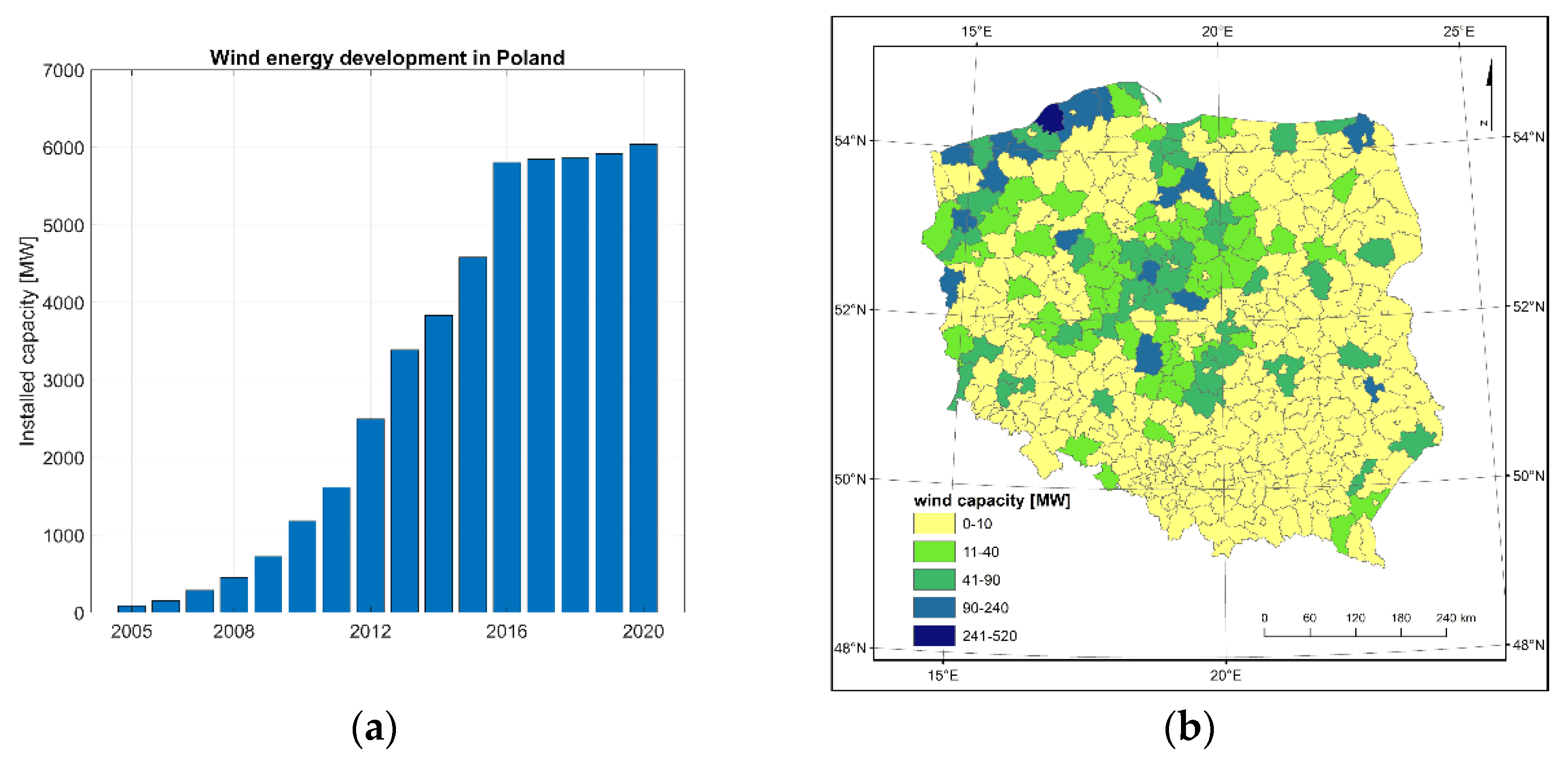
Hourly data time series of power generated on country level from wind turbines was obtained from Polskie Sieci Elektroenergetyczne (Polish Transmission System Operator). Together with information from Urząd Regulacji Energetyki (Energy Regulatory Office) about the localization and power of installed wind turbines in Poland, we constructed a database for every hour from 2018 to 2020 with power generated values and mean wind speed forecasts for County regions of Poland with installed wind turbines. From 2015 onwards, a stagnation in installed capacity in wind sources was observed (
Figure 3a), which provides a sizable learning sample for machine learning based methods. Additionally, dates from 2018 to 2020 were characterized with the most similar ALARO model characteristics (model version, physics configuration, boundary conditions), which is why this period was selected for this study. The majority of wind turbines in Poland are installed in the north and central parts of Poland (
Figure 3b).
3. Results
Results for all models are summarized in
Table 1 for hourly data and in
Table 2 for daily data of wind energy production. For hourly data, best results were obtained with the XGB model, with MAPE equal to 26.7% and RMSE 412 MW. The ANN method, with MAPE equal to 13.6% and RMSE 6481 MW, was the best for daily sums.
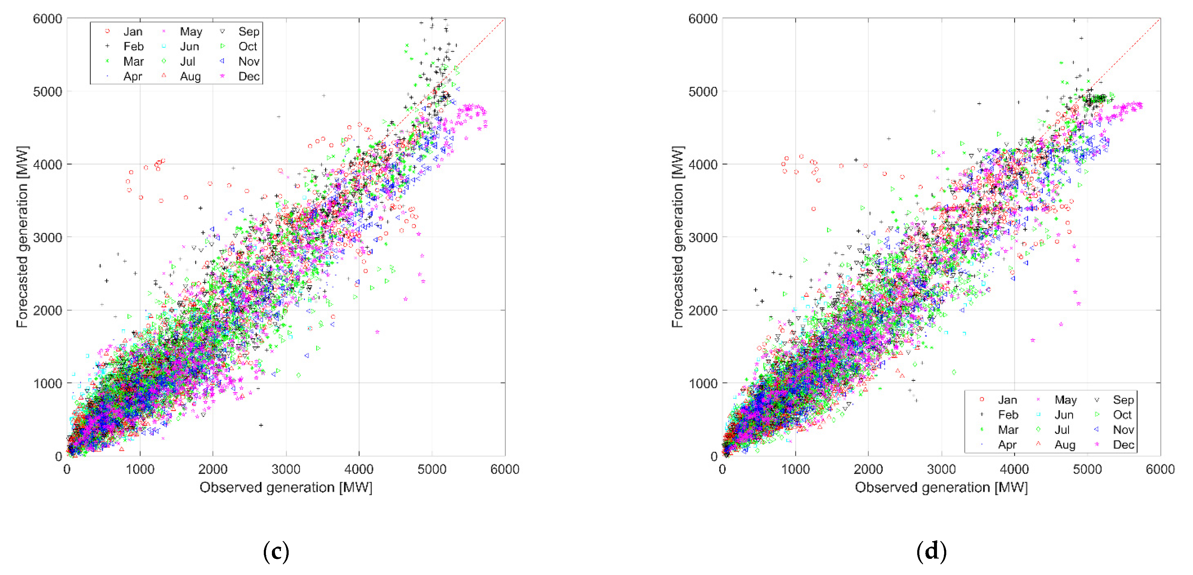
3.1. Scatterplots
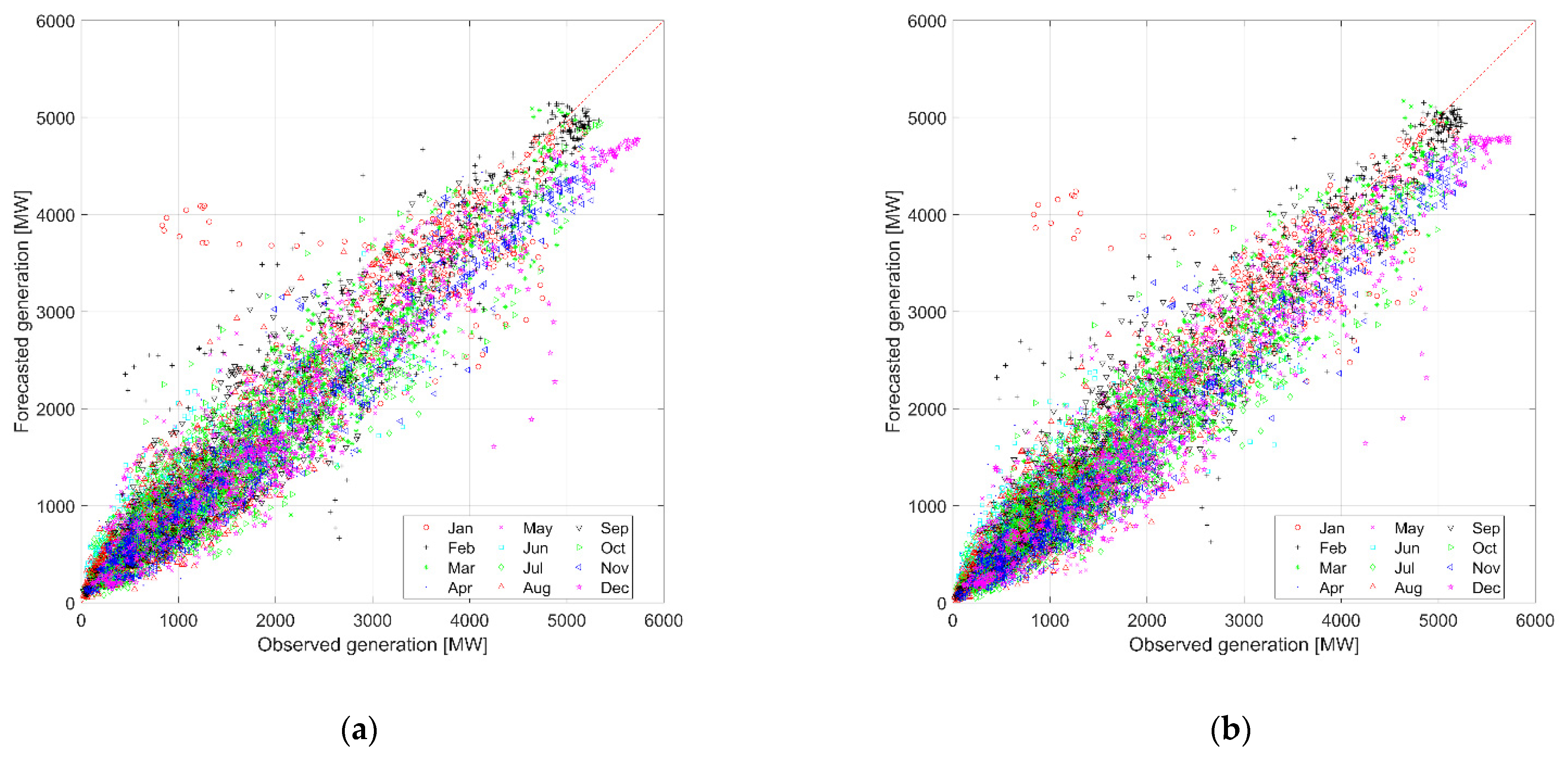
All models showed big seasonal differences in the results. In
Figure 4, prediction results are presented for all months in 2020, with biggest differences from observed values for winter and smallest errors in summer. Forecasted generation is overestimated for days in January (red dots) and February (black pluses). On the other hand, in December (pink stars), forecasts have the biggest underestimation. XGB and RF methods performed better than ANN and DNN, when there was very high real energy production.
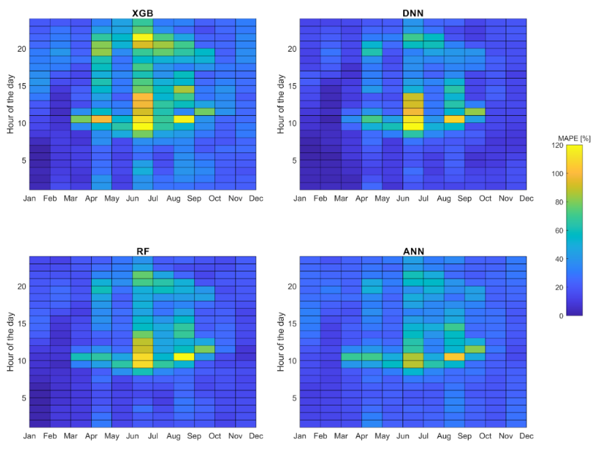
3.2. Hourly and Monthly Statistics
Hourly and monthly statistics of MAPE are presented in
Figure 5. For all models, the highest values (yellow colour) are present in June, while the lowest occurred in January and February (dark blue colour). Between 0 and 8 UTC, all models produced more accurate wind forecasts, which were represented by smaller MAPE. The ANN model had the lower variability of MAPE during days, as well as the whole year, while the XGB model has the highest differences between low error in January during nights and high error in July during days.
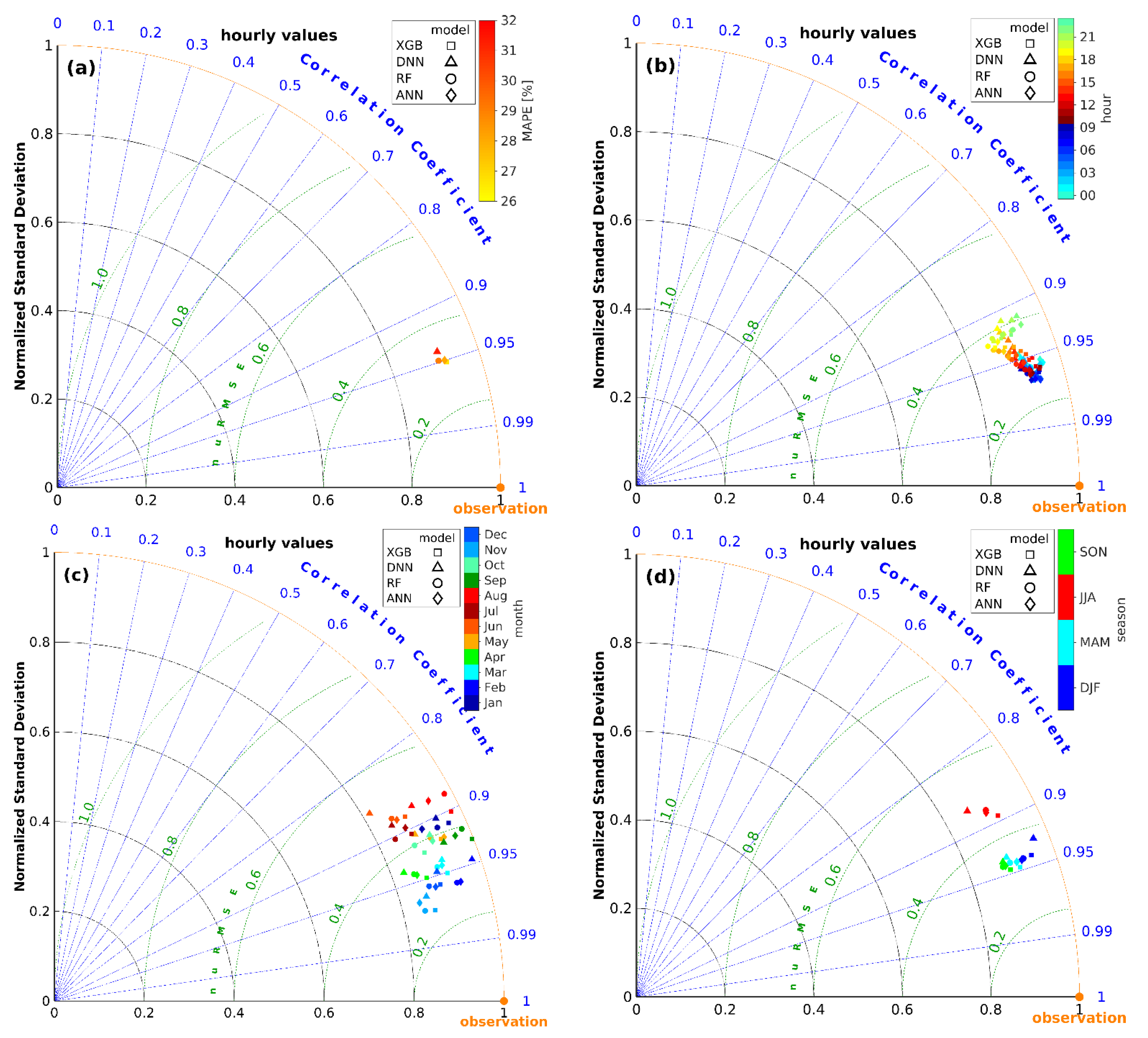
3.3. Taylor Diagrams
Taylor diagrams [
42] provide a concise statistical summary of agreement between modelled and observed data, in terms of their correlation, unbiased (or centered) root mean square error (uRMSE) and standard deviations. Additionally, the uRMSE is normalised (nuRMSE) to show relative dependence of statistics on hour, month and season. The statistics based on hourly data are shown in
Figure 6. All models (
Figure 6a) have good correlation values (about 0.95). The best agreement was found for the XGB model. RF and ANN models were slightly worse, and the DNN model was the worst. The same behaviour was seen for MAPE values, indicated as different marker colours. The statistics had a clear daily cycle (
Figure 6b). The best agreement is found in the morning, with a correlation value of about 0.97, variance closest to observational one and nuRMSE of about 0.25. Then, the correlation decreases, approaching nearly 0.9 and nuRMSE 0.4 in the late evening, but the variance is the most different from the observational one a bit earlier (15–18 UTC). The best correlation was found (
Figure 6c) in November (0.98) and in winter months (December and February, both 0.95) except January, and the worst in June and August (0.88). The hourly energy values for summer season had the worst reproducibility (
Figure 6d).
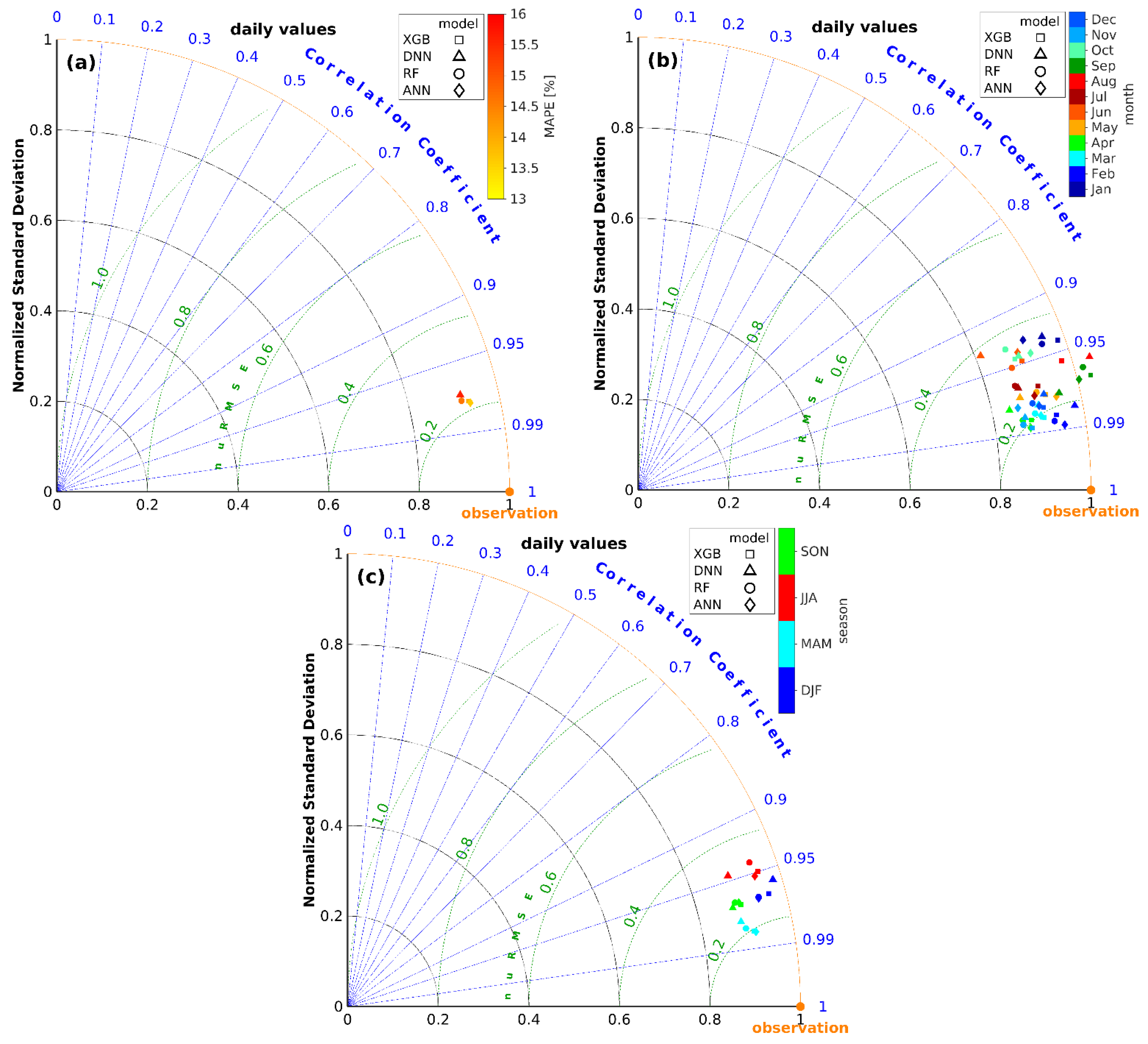
Verification statistics of model predictions for daily sums are shown in
Figure 7. All models agree very well (
Figure 7a), in terms of correlation (about 0.97). The ANN model was top-ranked, and the XGB model was slightly worse. The energy was very well-predicted in February, with correlation nearly 0.99 and standard deviation close to 1 (
Figure 7b), and the worst agreement was found in January. The diversity of winter months influenced seasonal behaviour (
Figure 7c). Modelled daily sums of produced energy were the best correlated with observations in spring. In autumn, the correlation was lower, but the variances were very similar in both seasons. Lower variance was found in winter, and the correlation was similar to spring’s values. The daily energy was worst predictable in summer.
It should be noted that MAPE values based on daily sums are about twice lower than those based on hourly data. One reason is that subdaily variability is hardly predictable.
3.4. Special Cases Study
Three special cases (mean errors of XGB model for 5 February 2020, 27 August 2020 and 27 December 2020 are presented in
Table 3) were selected from the testing period to show characteristic weather conditions with high and low wind energy prediction error. Weather charts in
Figure 8,
Figure 9 and
Figure 10 present meteorological situations over Europe, including fronts, air pressure systems, air masses, clouds, wind and temperature (available online
https://danepubliczne.imgw.pl/datastore).
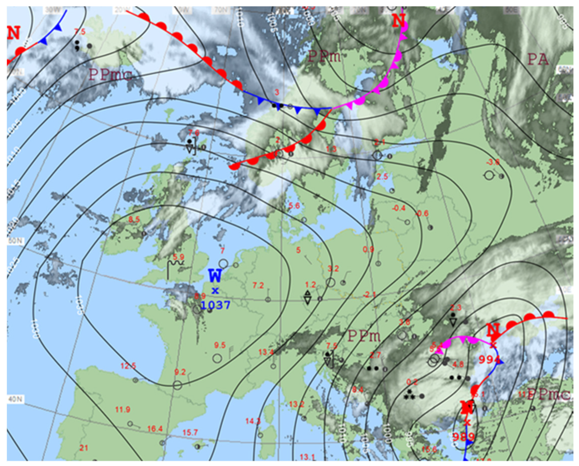
3.4.1. 5 February 2020
On 5 February 2020, a barometric ridge was located over Poland (
Figure 8). Wind was moderate, and airflow moved from the north and the northwest, following anticyclone circulation. Air masses were quite stable. Observed daily mean wind speed at the Polish weather station was around 4.0 ms
−1. On that day, the model estimated energy production very accurately. This result follows general findings for February, but, on the other hand, high late afternoon errors were also affirmed.
3.4.2. 27 August 2020
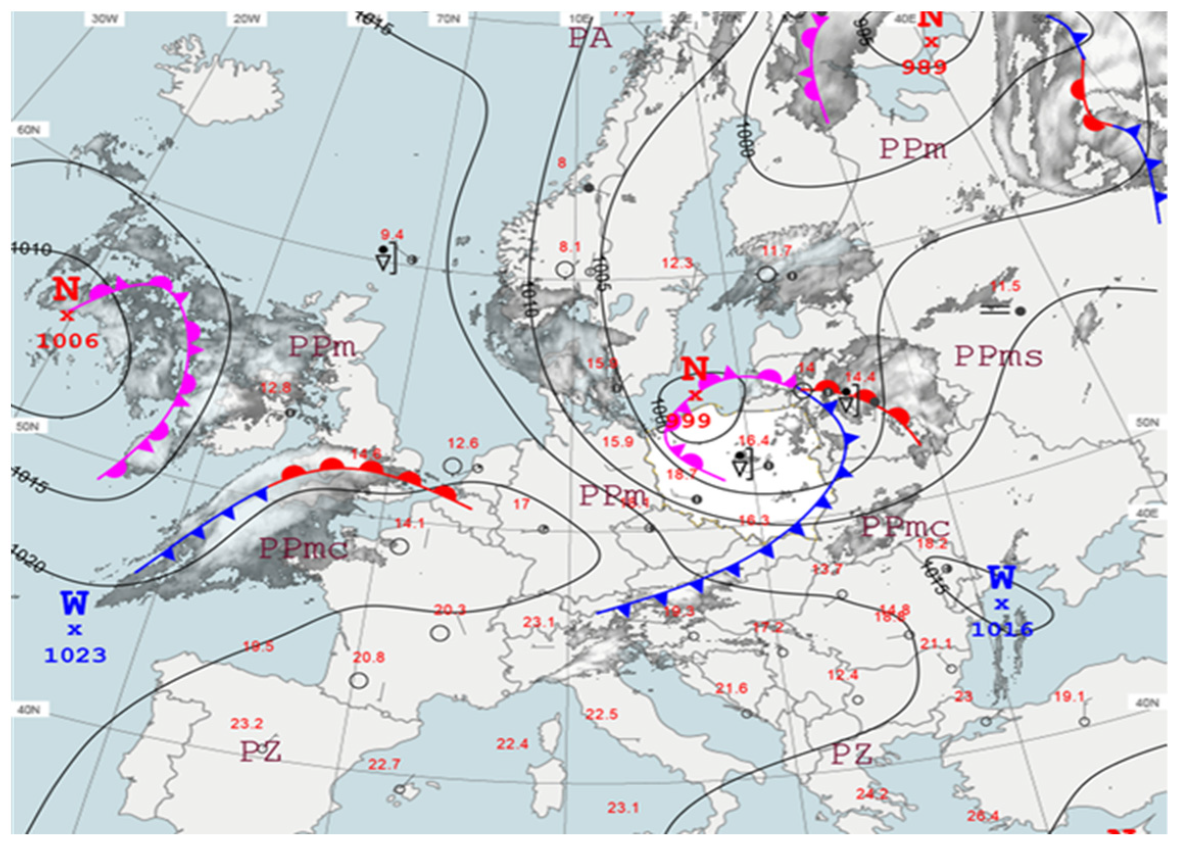
On 27 August 2020, as a result of a cold front that had passed the day before, unstable air above Poland moved eastward following north-western cyclonic circulation (
Figure 9). At the rear of the front, it was possible to observe thunderstorm phenomena. Sudden variations in wind speed were observed. At the centre of Poland (Toruń weather station), 10-min mean wind speed observation increased from 4.3 ms
−1 to 6.4 ms
−1 for 20 min (wind gust from 7.2 ms
−1 to 12.2 ms
−1). In the southwest of Poland (Wrocław weather station), mean wind increased from 4.8 ms
−1 to 7.5 ms
−1 (wind gust from 10.0 ms
−1 to 14.0 ms
−1). On that day, daily energy production was underestimated. It was also the case for nearly all hourly values.
3.4.3. 27 December 2020
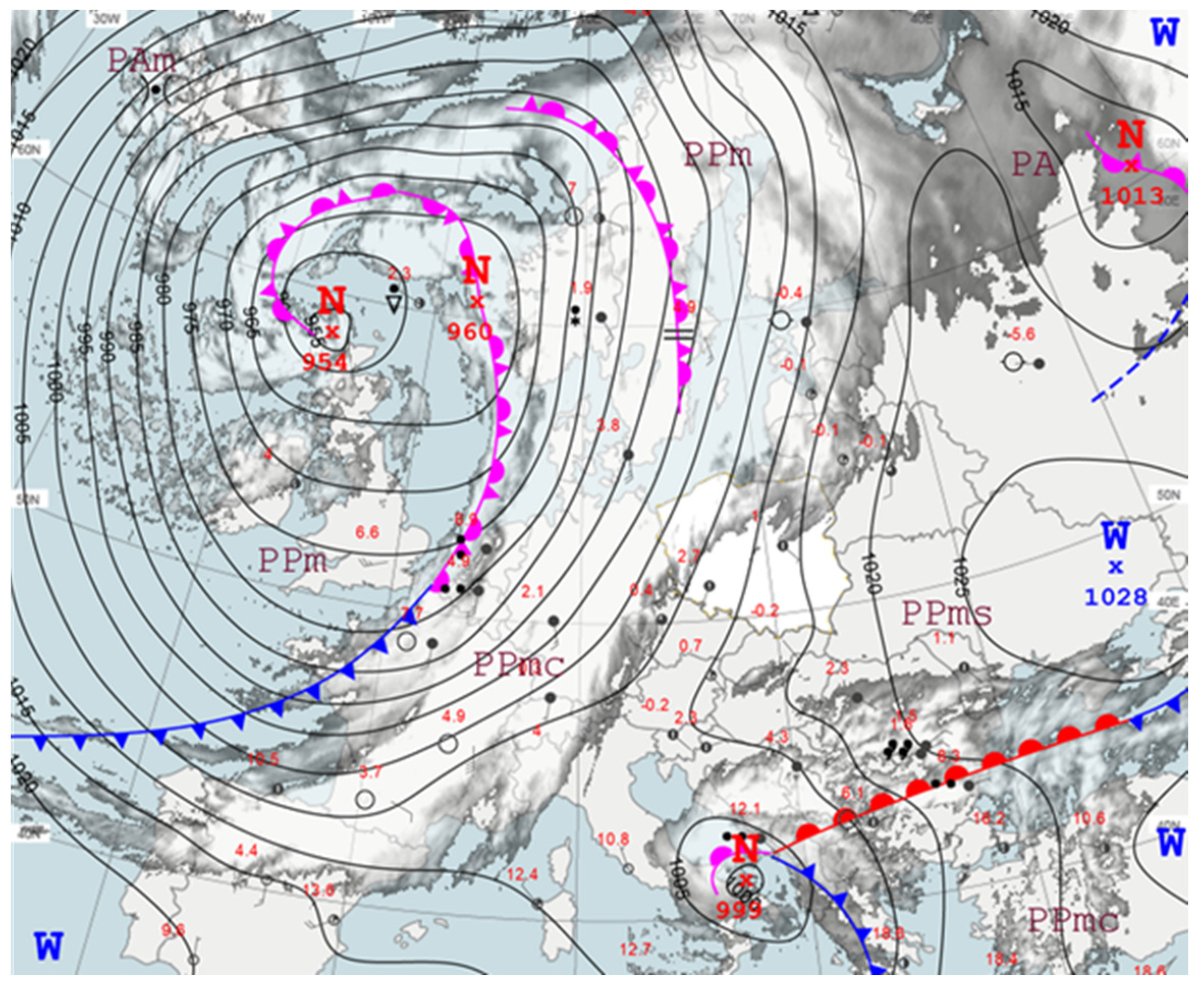
On 27 December 2020, Europe was dominated by a deepening low-pressure system above British Islands (954 hPa,
Figure 10) originating from a valley of the Rossby wave in the North Atlantic. A high-pressure system was located above east Ukraine. Surface low moved southeast, increasing atmospheric pressure gradient, causing strong south wind above Poland and fen-wind in the mountains. At the high-mountain weather station at Kasprowy Wierch, a maximum of 10-min mean wind speed was 20.4 ms
−1 (39.3 ms
−1 wind gust). Wind speed of 4.2 ms
−1 (10 ms
−1 wind gust) and 13.6 ms
−1 (20.2 ms
−1 wind gust) were observed in central (Warsaw) and northern Poland, seacoast (Łeba), respectively. Due to the large temperature gradient, thunderstorm phenomena were predicted for the next day, even though they are rare in December. On that day, the model overestimated hourly values of energy produced. 27 December 2020 was an exceptional day in production of electricity from Renewable Energy Sources (RES). The largest amount of electricity from wind was produced (5.7 GW), and the share of coal in electricity fell below 50%. Due to low electricity demand, its excess had to be exported to the Czech Republic.
4. Discussion
In this paper, we proposed a day-ahead wind power forecasting system based on multiple machine learning methods, an accurate limited area NWP model and hourly data time series of power generated from wind turbines that can be applied on the country level in Poland and possibly in other countries with similar climatological conditions. We have shown that all models (RF, XGB, ANN and DNN) produced forecasts with similar, high accuracy. The XGB model, with MAPE equal to 26.7% was the most accurate for hourly predictions, while for daily sums of produced energy, the ANN method, with MAPE equal to 13.6%, was the best. Our method, with forecasting wind energy production at national level and not for specific wind farms, has not been very often examined in the literature so far, so it is hard to compare our results with others’ research.
Although the comparison of machine learning methods was not the main topic of this publication, we have shown differences in terms of performance in different seasons, hours of the day and whether there is a high or low real energy production in the system. Results presented in the form of error metrics, scatterplots, tables and Taylor diagrams show that all presented methods can predict day-ahead wind power with high accuracy, although there are some differences in scores. Two methods based on decision trees (XGB and RF) were found to perform better than ANN and DNN in situations with very high hourly energy production. On the other hand, results of two methods based on neural networks (ANN ad DNN) are characterized with lower daily and monthly variability of MAPE. For all methods, June was the month with the highest and January with the lowest MAPE, while the lowest variances of results are found in winter months and the highest in summer.
Special cases were examined with both very accurate energy production forecasts and with big errors. In the stable weather conditions, with moderate wind speed, all models predicted wind energy production with high accuracy, but when the meteorological conditions are highly unstable or wind speed is extremely high, we can expect an increase of prediction errors. With the proposed method, the big impact on scores comes from accuracy of NWP forecasts. In a case study from 27 August 2020, when the convective system was present in the part of Poland with a high level of installed wind turbines, the overestimation of wind speed from the ALARO model resulted with high positive bias of energy production, especially in the evening hours. On the other hand, a case study from 27 December 2020 revealed a situation when very high wind speed in Poland was well-predicted by the ALARO model, but, due to known limitations of machine learning-based models, the extreme situations were usually underestimated. Another explanation might be switching off some wind turbines due to very high energy production. The third group of case studies are situations like the one presented on 5 February 2020, with moderate wind speed and stable conditions, when the proposed method performs well.
5. Conclusions
In this paper, we have shown that it is possible to predict a day-ahead wind energy production with high accuracy not necessarily by applying a physical or statistical model for every wind farm but by building machine learning based model with wind speed forecasts over the whole country. The proposed method needs an accurate NWP model and a long enough database with wind energy production and similar level of wind turbines installed on the examined area. Such vast area predictions are of big interest for planning energy production from conventional sources.
We believe that the same method can be applied to other countries, especially in Europe, but similar data must be available, especially hourly, country-level energy production. One of the limitations is that, in case of an increase of installed turbines in Poland, this method will have to be tuned, or a bias correction method will have to be applied. As this method is based on NWP results and machine learning methods, any major changes in the configuration of the used weather model will affect this method. In that case, a new version of the NWP model will have to be run again for a training period, and machine learning models must be trained on those forecasts. Another limitation is related to machine learning methods, themselves. In case of extreme weather conditions that were not present in the training dataset, results of this method may have unexpected errors.
In future work, we plan to work with more NWP models that are available in IMWM–NRI. We also intend to examine the effect on scores of adding more meteorological fields to our analysis (wind direction, temperature, humidity and pressure) and other methods that are often used, such as general regression neural network (GRNN) [
43,
44], radial basis function neural network (RBFNN) [
45], polynomial autoregressive model [
46] or SSOFC-Apriori-WRP [
47]. In the next step, we are planning to prepare an ensemble system based on multiple results that will not only give the best possible forecast but also produce probabilistic information, which will help in the decision-making process.
Author Contributions
Conceptualization, B.B., J.J. and M.F.; methodology, B.B., J.J. and A.J.; software, B.B., J.J. and G.S.; validation, T.S. and M.W.; formal analysis, B.B., J.J., A.J. and T.S.; investigation, J.J.; resources, P.S.; data curation, P.S. and T.S.; writing—original draft preparation, B.B., J.J., G.S., P.S. and M.W.; writing—review and editing, T.S. and M.F.; visualization, J.J., A.J. and T.S.; supervision, M.F.; project administration, M.F.; funding acquisition, M.F. All authors have read and agreed to the published version of the manuscript.
Funding
The study was performed as part of the research task “Development of forecasting methods to improve existing products and develop new application solutions, task 4. Implementation and development of methods of analysis and meteorological forecasting for the needs of renewable energy sources (S-6/2021)”, financed by the Ministry of Science and Higher Education (Poland), statutory activity of the Institute of Meteorology and Water Management-National Research Institute in 2021.
Data Availability Statement
Conflicts of Interest
The authors declare no conflict of interest.
Abbreviations
| ACCORD | A Consortium for Convection–Scale Modelling Research and Development |
| ALADIN | Aire Limitée Adaptation Dynamique Développement International |
| ALARO | ALADIN–AROME |
| ANN | Artificial Neural Network |
| AROME | Application of Research to Operations at Mesoscale |
| ARPEGE | Action de Recherche Petite Echelle Grande Echelle |
| CMC | Canonical Model Configuration |
| DNN | Deep Neural Network |
| ECMWF | European Centre for Medium-Range Weather Forecasts |
| HIRLAM | High Resolution Limited Area Model |
| IFS | Integrated Forecast System |
| IMWM–NRI | Institute of Meteorology and Water Management–National Research Institute |
| LAM | Limited Area Model |
| MAE | Mean Absolute Error |
| MAPE | Mean Absolute Percentage Error |
| nMAPE | normalized Mean Absolute Percentage Error |
| nRMSE | normalized Root Mean Square Error |
| NWP | Numerical Weather Prediction |
| RES | Renewable Energy Sources |
| RC-LACE | Regional Cooperation for Limited Area Modeling in Central Europe |
| RF | Random Forest |
| RMSE | Root Mean Square Error |
| nuRMSE | normalized unbiased Root Mean Square Error |
| uRMSE | unbiased Root Mean Square Error |
| XGB | Extreme Gradient Boosting |
References
- PSE Capital Group. Available online: https://www.pse.pl/ (accessed on 31 March 2021).
- Energy Regulatory Office. Renewable Energy Sources. Available online: https://www.ure.gov.pl/pl/oze/potencjal-krajowy-oze/5753,Moc-zainstalowana-MW.html (accessed on 31 March 2021).
- PSE Capital Group. Polish Power System-Report 2020. Available online: https://www.pse.pl/dane-systemowe/funkcjonowanie-kse/raporty-roczne-z-funkcjonowania-kse-za-rok/raporty-za-rok-2020#t1_1 (accessed on 31 March 2021).
- ENTSO-E Transparency Platform. Available online: https://transparency.entsoe.eu/ (accessed on 31 March 2021).
- Energy Market Information Center. National Electricity Demand in 2020. Available online: https://www.cire.pl/item,211874,1,0,0,0,0,0,krajowe-zapotrzebowanie-na-energie-elektryczna-w-2020-r.html (accessed on 31 March 2021).
- Renewable Energy Integration: Practical Management of Variability, Uncertainty, and Flexibility in Power Grids, 2nd ed.; Academic Press: Cambridge, MA, USA, 2017; pp. 1–462.
- El-Hendawi, M.; Wang, Z.L. An ensemble method of full wavelet packet transform and neural network for short term electrical load forecasting. Electr. Power Syst. Res. 2020, 182. [Google Scholar] [CrossRef]
- Kwon, B.S.; Park, R.J.; Song, K.B. Short-Term Load Forecasting Based on Deep Neural Networks Using LSTM Layer. J. Electr. Eng. Technol. 2020, 15, 1501–1509. [Google Scholar] [CrossRef]
- Liu, X.; Zhang, Z.J.; Song, Z. A comparative study of the data-driven day-ahead hourly provincial load forecasting methods: From classical data mining to deep learning. Renew. Sustain. Energy Rev. 2020, 119. [Google Scholar] [CrossRef]
- Jacobson, M.Z.; Delucchi, M.A. Providing all global energy with wind, water, and solar power, Part I: Technologies, energy resources, quantities and areas of infrastructure, and materials. Energy Policy 2011, 39, 1154–1169. [Google Scholar] [CrossRef]
- Hanifi, S.; Liu, X.L.; Lin, Z.; Lotfian, S. A Critical Review of Wind Power Forecasting Methods-Past, Present and Future. Energies 2020, 13, 3764. [Google Scholar] [CrossRef]
- Lin, Z.; Liu, X.L. Wind power forecasting of an offshore wind turbine based on high-frequency SCADA data and deep learning neural network. Energy 2020, 201. [Google Scholar] [CrossRef]
- Santhosh, M.; Venkaiah, C.; Vinod Kumar, D.M. Current advances and approaches in wind speed and wind power forecasting for improved renewable energy integration: A review. Eng. Rep. 2020, 2, e12178. [Google Scholar] [CrossRef]
- Zhang, Y.; Wang, J.X.; Wang, X.F. Review on probabilistic forecasting of wind power generation. Renew. Sustain. Energy Rev. 2014, 32, 255–270. [Google Scholar] [CrossRef]
- Yan, J.; Liu, Y.Q.; Han, S.; Wang, Y.M.; Feng, S.L. Reviews on uncertainty analysis of wind power forecasting. Renew. Sustain. Energy Rev. 2015, 52, 1322–1330. [Google Scholar] [CrossRef]
- Yang, M.; Shi, C.; Liu, H. Day-ahead wind power forecasting based on the clustering of equivalent power curves. Energy 2021, 218, 119515. [Google Scholar] [CrossRef]
- Zheng, D.; Shi, M.; Wang, Y.; Eseye, A.T.; Zhang, J. Day-ahead wind power forecasting using a two-stage hybrid modeling approach based on scada and meteorological information, and evaluating the impact of input-data dependency on forecasting accuracy. Energies 2017, 10, 1988. [Google Scholar] [CrossRef]
- Mana, M.; Astolfi, D.; Castellani, F.; Meißner, C. Day-ahead wind power forecast through high-resolution mesoscale model: Local computational fluid dynamics versus artificial neural network downscaling. J. Sol. Energy Eng. 2020, 142, 034502. [Google Scholar] [CrossRef]
- Shi, X.; Lei, X.; Huang, Q.; Huang, S.; Ren, K.; Hu, Y. Hourly day-ahead wind power prediction using the hybrid model of variational model decomposition and long short-term memory. Energies 2018, 11, 3227. [Google Scholar] [CrossRef]
- Augustyn, A.; Kamiński, J. A review of methods applied for wind power generation forecasting. Energy Policy J. 2018, 21, 139–150. [Google Scholar] [CrossRef]
- Rubanowicz, T. Power predictions methods of wind power plant. Sci. Pap. Fac. Electr. Control Eng. Gdańsk Univ. Technol. 2008, 25, 145–149. [Google Scholar]
- Popławski, T.; Dąsal, K.; Łyp, J. Problems related to forecasting of power and electric energy derived from wind. Energy Policy J. 2009, 12, 511–523. [Google Scholar]
- Karkoszka, K. Forecasting methodologies of the electrical power generation from wind farms for the purpose of operation and balancing of power systems. Bull. Miner. Energy Econ. Res. Inst. Polish Acad. Sci. 2010, 78, 75–86. [Google Scholar]
- Baczyński, D.; Piotrowski, P. A one day ahead forecasting of twenty-four-hour electric energy production for wind turbine. Prz. Elektrotechniczny 2014, 9. [Google Scholar] [CrossRef]
- Popławski, T.; Szeląg, P. Use of Hurst exponent to predict instability of wind generation. Rynek Energii 2014, 5, 116–120. [Google Scholar]
- Szeląg, P. Forecasting wind generation in the context of energy resurces management. Energy Policy J. 2014, 17, 125–134. [Google Scholar]
- Hossa, T.; Sokołowska, W.; Fabisz, K.; Filipowska, A. Forecasting wind power generation using local methods and the nonlinear regression. Rynek Energii 2014, 2, 61–68. [Google Scholar]
- Rubanowicz, T. Wind Power Generation Forecasting; Gdańsk University of Technology: Gdańsk, Poland, 2019. [Google Scholar]
- Malska, W.; Mazur, D. Analysis of the impact of wind speed for power generation on the example of wind farm. Przegląd Elektrotechniczny 2017, 93, 54–57. [Google Scholar] [CrossRef]
- Baczyński, D.; Kopyt, M. Quality analysis of wind turbines electrical energy production forecasts based on UM and COAMPS meteo data. Przegląd Elektrotechniczny 2017, 93, 171–175. [Google Scholar] [CrossRef]
- Czapaj, R.; Szablicki, M.; Rzepka, P.; Sołtysik, M. Short-term forecasting of demand and generation profiles in energy clusters. Przegląd Elektrotechniczny 2019, 95, 137–140. [Google Scholar] [CrossRef]
- Popławski, T.; Szeląg, P. Use of fractal analysis and adaptive curve for short-term power forecasts of wind farms. Rynek Energii 2020, 1, 25–30. [Google Scholar]
- Pietrzak, M.; Świderski, J. Short-term weather forecasting concept for the energy sector. Rynek Energii 2020, 4, 32–37. [Google Scholar]
- Breiman, L. Random forests. Mach. Learn. 2001, 45, 5–32. [Google Scholar] [CrossRef]
- Liaw, A.; Wiener, M. Classification and Regression by RandomForest. Forest 2001, 23, 18–22. [Google Scholar]
- LeCun, Y.; Bengio, Y.; Hinton, G. Deep learning. Nature 2015, 521, 436–444. [Google Scholar] [CrossRef] [PubMed]
- H2O.ai. Available online: https://www.h2o.ai/ (accessed on 31 March 2021).
- Chen, T.Q.; Guestrin, C.; Assoc Comp, M. XGBoost: A Scalable Tree Boosting System. In Proceedings of the 22nd Acm Sigkdd International Conference on Knowledge Discovery and Data Mining, San Francisco, CA, USA, 13–17 August 2016. [Google Scholar] [CrossRef]
- Boehmke, B.; Greenwell, B.M. Hands-On Machine Learning with R; Taylor & Francis: Milton Park, UK, 2019. [Google Scholar]
- Termonia, P.; Fischer, C.; Bazile, E.; Bouyssel, F.; Brozkova, R.; Benard, P.; Bochenek, B.; Degrauwe, D.; Derkova, M.; El Khatib, R.; et al. The ALADIN System and its canonical model configurations AROME CY41T1 and ALARO CY40T1. Geosci. Model Dev. 2018, 11, 257–281. [Google Scholar] [CrossRef]
- Bochenek, B.; Sekuła, P.; Jerczyński, M.; Kolonko, M.; Szczęch-Gajewska, M.; Woyciechowska, J.; Stachura, G. ALADIN in Poland. In Proceedings of the 41th EWGLAM and 27rd SRNWP Online Meeting, 28 September–2 October 2020; Available online: srnwp.met.hu/Annual_Meetings/2020/download/posters/poster_poland_ALADIN_EWGLAM2020.pdf (accessed on 31 March 2021).
- Taylor, K.E. Summarizing multiple aspects of model performance in a single diagram. J. Geophys. Res. Atmos. 2001, 106, 7183–7192. [Google Scholar] [CrossRef]
- Liang, Y.; Niu, D.; Hong, W. Short term load forecasting based on feature extraction and improved general regression neural network model. Energy 2019, 166. [Google Scholar] [CrossRef]
- Niu, D.; Wang, H.; Chen, H.; Liang, Y. The General Regression Neural Network Based on the Fruit Fly Optimization Algorithm and the Data Inconsistency Rate for Transmission Line Icing Prediction. Energies 2017, 10, 2066. [Google Scholar] [CrossRef]
- Hong, Y.Y.; Rioflorido, C.L.P.P. A hybrid deep learning-based neural network for 24-h ahead wind power forecasting. Appl. Energy 2019, 250, 530–539. [Google Scholar] [CrossRef]
- Karakuş, O.; Kuruoğlu, E.E.; Altınkaya, M.A. One-day ahead wind speed/power prediction based on polynomial autoregressive model. IET Renew. Power Gener. 2017, 11, 1430–1439. [Google Scholar] [CrossRef]
- Li, L.; Yin, X.L.; Jia, X.C.; Sobhani, B. Day ahead powerful probabilistic wind power forecast using combined intelligent structure and fuzzy clustering algorithm. Energy 2020, 192, 116498. [Google Scholar] [CrossRef]
| Publisher’s Note: MDPI stays neutral with regard to jurisdictional claims in published maps and institutional affiliations. |
© 2021 by the authors. Licensee MDPI, Basel, Switzerland. This article is an open access article distributed under the terms and conditions of the Creative Commons Attribution (CC BY) license (https://creativecommons.org/licenses/by/4.0/).


 ,
, 


