Article

Leveraging Label Information in a Knowledge-Driven Approach for Rolling-Element Bearings Remaining Useful Life Prediction

by
Tarek Berghout
1,
Mohamed Benbouzid
2,3,* and
Leïla-Hayet Mouss
1
1
Laboratory of Automation and Manufacturing Engineering, University of Batna 2, Batna 05000, Algeria
2
Institut de RechercheDupuy de Lôme (UMR CNRS 6027), University of Brest, 29238 Brest, France
3
Logistics Engineering College, Shanghai Maritime University, Shanghai 201306, China
*
Author to whom correspondence should be addressed.
Energies 2021, 14(8), 2163; https://doi.org/10.3390/en14082163
Submission received: 28 March 2021 / Revised: 6 April 2021 / Accepted: 11 April 2021 / Published: 13 April 2021
(This article belongs to the Special Issue Failure Diagnosis and Prognosis of Induction Machines)

Abstract

:
Since bearing deterioration patterns are difficult to collect from real, long lifetime scenarios, data-driven research has been directed towards recovering them by imposing accelerated life tests. Consequently, insufficiently recovered features due to rapid damage propagation seem more likely to lead to poorly generalized learning machines. Knowledge-driven learning comes as a solution by providing prior assumptions from transfer learning. Likewise, the absence of true labels was able to create inconsistency related problems between samples, and teacher-given label behaviors led to more ill-posed predictors. Therefore, in an attempt to overcome the incomplete, unlabeled data drawbacks, a new autoencoder has been designed as an additional source that could correlate inputs and labels by exploiting label information in a completely unsupervised learning scheme. Additionally, its stacked denoising version seems to more robustly be able to recover them for new unseen data. Due to the non-stationary and sequentially driven nature of samples, recovered representations have been fed into a transfer learning, convolutional, long–short-term memory neural network for further meaningful learning representations. The assessment procedures were benchmarked against recent methods under different training datasets. The obtained results led to more efficiency confirming the strength of the new learning path.

1. Introduction

A successful conditional preventive maintenance program relies entirely on precise real-time monitoring, is capable of prior detection of any failure suspicion, and stands on a well-structured prognosis policy [1]. Remaining useful life (RUL) is very crucial for prognosis, taking place as the primary measure of health assessment [2]. It is mainly based either on the estimation of useful time until the complete failure of such a system or on the provision of a probability or any other important information indicating its current operational performance. Its evaluation involves the use of different modeling paradigms, depending on the complexity of the system as well as the availability of the operating history, including all anomaly events [3]. If it is not difficult to represent the operating behavior using physical interpretations, then it would be a very authentic modeling process that could certainly lead to an accurate RUL prediction. Likewise, data-driven evaluation is a very common promising solution in case of unavailability of the physical modeling process. In data-driven training procedures, the precise RUL estimation process depends on two main characteristics, namely: (i) complete run-to-failure historical sensor measurements, and (ii) truly attributed labels to each event. However, for some machines such as bearings, collecting these large deterioration patterns seems most likely impossible due to their long lifetime. Conversely, it seeks to recover patterns of progressive damage propagation by imposing accelerated life tests to collect patterns similar to the real ones as an alternative solution. Moreover, even if these data are stored correctly, the real labels are still missing, and the short lifespan could not be considered as a ground truth label.
This unavailability of truly assigned labels leads prognosis-based data-driven research to estimate the RUL by providing sufficient interpretations from the operating history. There are two main indicators involved in providing the operating performance and the level of criticality belonging to this operating mode (e.g., critical, healthy, deteriorating, etc.) [4]. One of these indicators is the health index (HI), which is based on determining the probability that the system will be able to function within a certain period of time [4]. The other is the health stage (HS), which consists of determining the thresholds that can divide the life path into several levels, indicating the part to which the current performance belongs [4]. In doing so, the question “What are the current performances of this system? Is this critical?” will be fully answered and a consistent conclusion about the RUL will be obtained.
In the literature, the determination of HS can be performed by one of the two following tools; intelligent machine learning (ML) tools, such as clusters, or via signal processing techniques (SP). Intelligent ML tools help in multiple clustering processes based on well pre-preprocessed data [5]. Conversely, HS splitting with SP techniques generally involves the detection of a single threshold, namely, the “failure threshold”, which is most likely similar to fault classification (diagnosis not prognosis) [6,7,8]. For instance, in the work of Ben Ali, J. et al. [9], RUL of the bearing prediction process was performed only through HS identification using the intelligent maintenance systems (IMS) bearing data set. The SP technique, namely, the empirical mode decomposition (EMD), is involved as the main indicator of the HS. In the meantime, principal component analysis (PCA) and linear discriminate analysis (LDA) are used for feature reductions before feeding them in a probabilistic artificial neural network (ANN). In another work [10] related to the bearing degradation prognosis of wind turbine high-speed shaft (WTHS) [11], they followed the same methodology to predict RUL. However, this time they involved multiple extracted time-frequency features to train an unsupervised neural network, namely, adaptive resonance theory 2 (ART2), for feature clustering. Khamoudj, C.E.et al. [5] used a multiple clustering process that involves the variable neighborhood search (VNS) algorithm. Their work mainly depends on bearing RUL prediction by exploiting multiple levels of HS. Han, S. et al. [12] replicated the same experiments in [9] using an already split version of the IMS dataset into multiple HS levels. Their main contribution involves a powerful multi-scale convolutional neural network (CNN) for feature classification. Moshrefzadeh, A. et al. [13] investigated the use of two methods, support vector machine (SVM) and k-nearest neighbors, for feature clustering and HS classification for multiple datasets including IMS bearings. Additionally, signal impulsiveness has been employed as the main health indicator in the online prognosis system under multiple operating conditions. Zareapoor, M. et al. [14] investigated the use of a new adversarial classification algorithm for both HS and HI predictions to solve imbalanced data problems. However, their contribution on IMS bearing data that include only the HS splitting process proves its capability compared to other data-driven approaches.
These mentioned works have shown their success by answering the second part of the previous question, in which it can give an idea of the level of health. However, the full answer to the first part is not yet provided. Accordingly, some works have been done on the HI predictions to provide a reliable conclusion about the health status. In general, the HI estimation is fully data-driven, and it depends on the approximation of the training model towards a linearly deteriorated probability function. Under this criteria, Saidi, L. et al. [15] posted an experiment related to the same RUL prediction issue from the WTHS dataset. However, this time, they investigated the HI prediction problem using spectral kurtosis (SK) and support vector regression (SVR). Meddour, I. et al. [16] extracted 30 features from acceleration signals from time, frequency, and time–frequency domains in an attempt to realize an accurate HI prediction for the same WTHS data. They incorporated, therefore, an adaptive ANN and fuzzy inference system for the approximation process towards a linear deterioration function of HI. Li, X. et al. [17] studied both HI and HS under the use of different dataset-related bearing prognosis problems. They mainly involved deep generative adversarial models to perform more generalization. Wang, J.et al.[18] used a prognosis learning approach to deal with a limited set of data by incorporating wavelet transform, statistical Bayesian framework, and recursive filtering for feature extraction and HI prediction, respectively.
One may notice that the above-mentioned works with their different architectures and prediction techniques, including both SP and ML techniques, have been very successful at achieving their maximum accuracy. However, they still suffer from the lack of patterns related to incomplete data, leading to poor generalization. Therefore, knowledge-driven research comes as a solution by providing additional assumptions from previously-trained learning machines. In this context, many recent works have been released in the area of transfer learning (TL), especially for bearing health assessments. Huang, G. et al. [19] developed a TL approach that incorporates a serially connected CNN and long–short-term memory (LSTM) for HI index estimation only. They mainly discussed the use of two different bearing datasets, including the IMS bearing set. In the work, Kim, M. et al. [20], in an attempt to overcome drawbacks produced by the insufficiency and discrepancy related to collected samples, designed a TL approach that followed adaptation with a semantic clustering mechanism. Clustering results, thereafter, have been fed into a target domain CNN to achieve better HS classification of bearing life cycles. Zhuang, F. et al. [21] developed a TL-based CNN for bearing RUL predictions under different operating conditions. Their main contribution involved an accurate approximation towards a linearly designed HI by transferring knowledge from different subsets of bearing life cycles.
According to this brief review, TL proved its capability by filling the gaps of lack of patterns leading to further generalization [22]. However, even after all these efforts, we still face many types of ill-posed problems leading to false predictions, especially if the data suffer from higher levels of similarity between the training samples, as in vibration signals. In addition, we believe that the behavior of the HI, which is defined according to expert knowledge depending on the deterioration type (linear or exponential), could also create problems resulting from incompatibility with the behaviors of the learning patterns.
Attempting to overcome these poor generalizations and weaknesses in approximation related problems, a few works have been recently proposed. For instance, the works of Sánchez-Morales A. et al. [23,24] and Berghout, T. [25] clearly proved the necessity of exploiting label information in data-driven modeling. To the best of our knowledge, these works are the only ones who deal with this kind of representation learning scheme as a knowledge-based prior assumption. However, they seem to be totally dependent on previously trained learners (regressors or classifiers), which might also be inaccurate enough to seed deceptive patterns in the representation learning features. Furthermore, their obtained labels from these auxiliary learners have been seeded in the inputs themselves, which could lead to corruption of important patterns.
Accordingly, in the context of bearing diagnosis and to make sure that all the above prediction issues have been well considered, our main propositions for bearing RUL predictions are as follows:
  • A new autoencoder (AE) capable of seeding label information in hidden layers without affecting the learning inputs or even the reconstruction process, and also to ensure knowledge transfer, is designed.
  • This AE is stacked and strengthened with a denoising scheme to ensure more robust extraction as well as more homogeneous mixture of label and feature mapping.
  • Due to the sequentially driven and non-stationary nature of vibration signals, a convolutional LSTM (C-LSTLM) has been designed to fit both time-varying adaptive learning as well as accurate extraction, similar to the work done in [26].
  • Two main datasets, namely, IMS and WTHS, have been involved in an attempt to produce more generalization by transferring knowledge between them using the same learning framework.
  • Unlike previously mentioned works that mostly deal with a single prediction problem (either HI or HS), both HI and HS have been investigated in this work.
  • In this work, we also used an exponential HI deteriorating function that shows it is more compatible with extracted deterioration features rather than the linear one.
  • Concerning the HS splitting, we have involved the Gaussian mixture model (GMM) based silhouettes coefficient.
The reminder of this paper is organized as follows: in Section 2, the studied bearing datasets and the proposed methodology have been described. Section 3 is devoted to experimental results and discussions. Section 4 concludes with perspectives.

2. Materials and Methods

This section provides important descriptions related to the used datasets in this work (IMS bearing and WTHS), as well as the details of the followed methodology during RUL prediction.

2.1. IMS Bearing Data

First, the IMS bearing dataset was made available by IMS of University of Cincinnati [11]. Since then, it was provided by NASA at a prognostic data repository for the public to be able to evaluate their health assessment models [27]. The experiment incorporated four bearings aligned with a single feed shaft (Figure 1) with 6000 pounds and a speed of 2000 rpm.
The IMS data contained three subsets, the first of which was released from two installed accelerometers. In the meantime, the other two sets were brought together from a single sensor. Data acquisition was performed with a sampling rate of 20 kHz where each file was stored separately every second. This means that each file could contain at least 20,000 samples, which can be considered very difficult to manipulate for training models as a single observation. For each experiment, the associated files were gathered in a single folder and named after the date and time of acquisition. The vibration signals in Figure 2 show how bearing health deteriorates over time in each experiment. The bearing tests lasted approximately 35 days until the appearance of certain significant symptoms of bearing failure.

2.2. WTHS Bearing Data

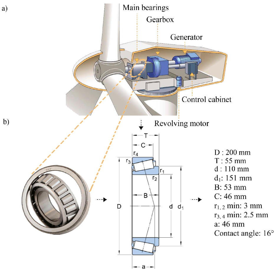
In an attempt to obtain more realistic conclusions from the analysis of bearing deterioration, an experiment was carried out to record the real-time health indicators of a high-speed shaft with 20 tooth pinion gear driven by 2 MW wind turbine. Figure 3 is a simple graphical illustration of the studied system that indicates the position of the main bearings as well as the dimensions of the taper roller bearings.
The vibration measurements were recorded by an actual designated monitoring system in the United States [10]. A single accelerometer was installed perpendicular to the high-speed shaft in the gearbox bearing to be able to detect the progressive spread of damage. The monitoring system was programmed to store 6 s of vibration samples each day with a sampling rate equal to 100 kHz. Fifty files were stored separately for 50 days where an amount of approximately 585,936 samples per file was treated as a single health indicator [28]. It was observed that the collected data varied exponentially over time due to the changes that occurred in the physical health conditions of the bearings, as shown in Figure 4. Consequently, within 50 days under normal operating condition, the bearings stopped working due to the occurrence of an internal race fault.

2.3. Proposed Knowledge-Driven Methodology

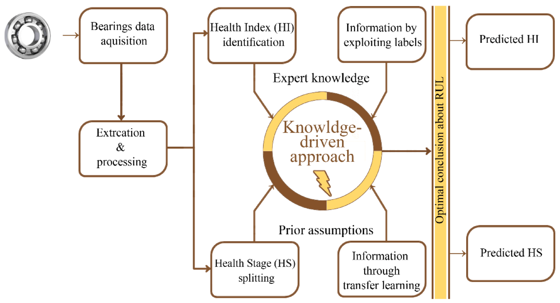
In order to provide a more reliable conclusion on the RUL prediction of such a system, a new methodology, which involves multiple sources of knowledge, has been involved in a unique learning scheme that is designed according to the flow diagram enshrined by Figure 5. Both data-driven and knowledge-driven methodology have been utilized, along within this new learning procedure, by exploiting TL information, deep learning labels, as well as previous hypotheses generated from pre-trained models.

2.3.1. Data Preprocessing

To guarantee an optimal feature space for representation learning algorithms, a well-structured feature extraction was considered. In total, 15 statistical features were extracted from both time-domain and frequency-domain for both datasets.
Eleven time-domain features were calculated for each time window (mean, standard deviation (Std), skewness, kurtosis, peak to peak indices (Peak2Peak), root mean squared (RMS), crest factor, shape factor, impulse factor, margin factor energy} in addition to four frequency-domain features {spectral kurtosis mean (SKMean), SKStd, SKSkewness, SKKurtosis}. More information about the mathematical background of these features can be obtained from [10]. After that, these parameters were scaled in the interval 0 , 1 using min–max normalization and fed directly into the learning models. Regarding smoothness filtering procedures of the extracted features, as in [27], we do not think they will be beneficial. In fact, this may be applicable in this case if the training and testing data is pre-defined. However, in a real application, one cannot guess how far we could scale our samples, especially when the newly arrived samples are driven one-by-one. Therefore, by trying to avoid any misleading representations, we both trained and tested the learning models by samples as they resulted from min–max normalization.
Figure 6 illustrates the behavior of the entities extracted from the two datasets. It can be seen that the WTHS dataset exhibited a complete data deterioration lifecycle, which seemed very adequate for the learning process in terms of the compatibility of the degradation form. Conversely, the IMS dataset was more difficult because it could lead the training program to expose all kinds of ill-posed problems.

2.3.2. HI Identification

Unlike traditional works, which present the deterioration path as a linear function; in our work we used an exponential function, which is illustrated by Equation (1), that seems more adaptable with the approximation process. The similarity between the shape of the deterioration and the exceptional function of degradation creates a kind of compatibility between the labels and the extracted patterns.
H I t =   d + e a t + b .
t   stands for the time instant, and   a , b , d are hyperparameters that control the divergence characteristics of the exponential degradation. These parameters are tuned according to the best results of the loss function. Figure 7 is an illustrative example indicating the HI identification process for the two studied datasets.

2.3.3. HS Splitting

Among many clustering machines, we have chosen to use the Gaussian mixture model (GMM) to divide the training patterns according to three distinct operating phases of bearings (healthy, deteriorated, critical). The reasons for this choice lie in the learning procedures of GMM, which use more statistical characteristics, such as the mean and standard deviation, than others, such as K-nearest neighbor (KNN) variants [5], which use only the mean value for subspaces-divisions. The KNN variants divide the data into subspaces by identifying the circular boundaries centered in the medal of each class with a radius equal to the mean value of the samples of that class. On the other hand, GMM is able to provide more flexibility and smoothness by providing an ellipsoidal shape to the decision classes [29,30]. In GMM, clustering probability can be defined as expressed by Equation (2).   x refers to the training sample, λ = x , u , Σ are the statistical components of the GMM model, and u , Σ are the mean and variance, respectively.
P ( x | λ ) = i = 1 n w i g ( x | u i , Σ i ) ,
Each clustering component can be defined as expressed by Equation (3). Where D stands for the number of features in each observation (e.g., in our case, we have 15 features).
g x | u i , Σ i = 1 2 π D / 2 e 1 2 x μ i Σ i 1 x μ i .
Since clustering is an unsupervised learning process, it is, therefore, very difficult to judge whether the model is really able to classify the data correctly or not due to the lack of ground truth labels. However, we are still able to guess whether the model is able to group this kind of data at certain numbers of classes or not. For instance, in our work, we used Silhouette analysis for this mission. The Silhouette coefficient is a metric that can be used to measure the amount of groups that such a cluster is able to detect [31]. Equation (4) illustrates the measurement of this parameter α using only the largest and the smallest average distances between learning samples ω , γ , respectively.
α = ω γ max ω , γ .
In our work, this simple test proves that GMM is really capable of doing it under these datasets, as shown in Figure 8.

2.3.4. Denoising Autoencoder for Label Embedding

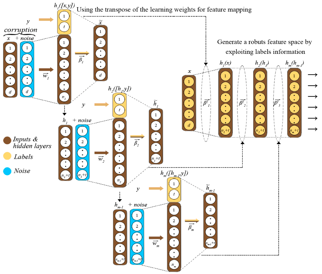
In the proposed learning scheme, the integration of labels was carried out via a stack of autoencoders connected in series. The main objective was to seed patterns similar to the labels in the learning representations of the hidden layers of the neural network. We believe the more the shape of the inputs reflects the targets, the more the approximation will do (as it will be experimentally proven later). As we can see from the illustrations in Figure 9, the denoising scheme was incorporated to strengthen the representations, attempting to lead to more meaningful patterns. Additionally, the stack of autoencoders was designed to homogenize the labels as much as possible with the original mapped patterns without distorting them.
Due to the local connections between the hidden layer and the input layer resulting from additive labels, also due to the deep complex architecture, we moved forward using a tuning algorithm on one side capable of adjusting only the output weights accurately and quickly. To the best of our knowledge, the only algorithm capable of doing so is the extreme learning machine (ELM)[32]. Therefore, the learning steps of the proposed stacked denoising autoencoder with embedded labels (SD-AEEL) can be presented as follows:
  • Retrieve corrupted inputs x η using generated noise from any distribution with a specific magnitude ζ and rate ψ and use them to corrupt the inputs x , same as in Equation (5).
    x η = η x , ζ , ψ ,
  • Activate the hidden layer h using any activation transfer function f that holds both ordinary full rank mapping of x η   and seeded labels y   , as explained by Equation (6). w , b are the input weights and biases, respectively.
    h x η = f w x η + b , y ,
In fact, Equation (6) is our main contribution in this work, and as far as we know, it is the only one of its kind.
  • Determine the reconstructions weights β using the original inputs and the new feature mapping, same as described by Equation (7).
    β = x h 1 ,
  • Repeat the learning process by considering the hidden layers as inputs of the next autoencoders, as explained by Equation (8), where m is the index of the autoencoder.
    x m + 1 = h m ,
  • After the training process is finished, one can construct a fully trained network for robust feature mapping using the transpose of the output weights β T , as in Equation (9).
    h x = x β T .

2.3.5. Data-Driven Network and Transfer Learning

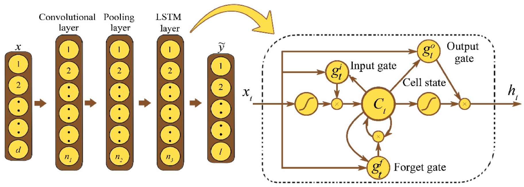
The showcased convolutional LSTM (C-LSTM) network in Figure 10 represents the main data-driven approach used for both training in source domain and knowledge transfer to the target domain. As we can see, it consists of three main layers; the convolutional layer, the pooling layer, and the LSTM layer.
In the convolutional layer, the training samples were mapped through local dimensional (1D) receiver filters into several hierarchical slices. Following that, each resulting slice of the entity mapping was sub-simplified using maximum pooling. In addition, the pooling layer was introduced in the LSTM layer for approximation and generalization. Regarding the TL process, the learning weights of C-LSTM were used to provide further generalization for the learning models in the target domain.
The reason we chosethe LSTM network was due to its powerful capability in adaptive sequential learning without suffering from vanishing gradient problems [33]. It uses a set of learning gates, namely; input gate g t i , forgetting gate g t f , and output gate g t o ,to control the amount of memorization of any driven patterns, as demonstrated by Equations (10)–(12).
g t i = f w i h t 1 + x t + b i ,
g t f = f w f h t 1 + x t + b f ,
g t o = f w o h t 1 + x t + b o ,
In the meantime, the hidden state   h t and the cell state   C t are initially determined using Equations (13)–(15).
h t = f w h h t 1 + x t + b h ,
C ˜ t = f w c h t 1 + x t + b c ,
C t = g t f C t 1 + g t i C ˜ t 1 .

3. Results and Discussion

This section provides results and discussion related to the performances of the designed algorithm, starting with label seeding towards both HI and HS predictions.

3.1. Labels Recovering Process

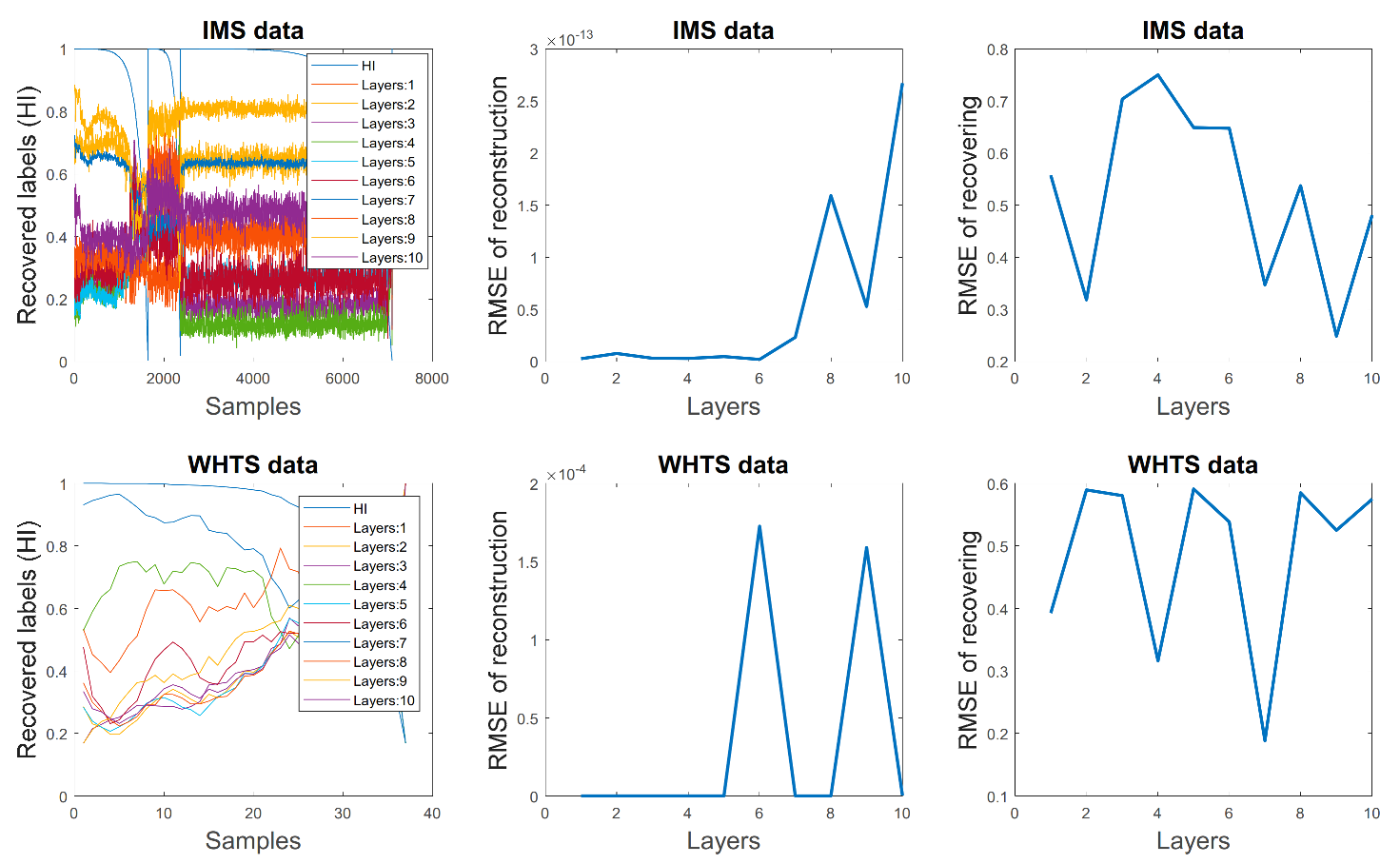
Unlike traditional unsupervised learning autoencoders that follow the input reconstruction path, our designed stacked denoising version is able to perform two main tasks simultaneously, namely, label regeneration and input reconstruction. Therefore, to prove this ability to keep the inputs as is without affecting them in any way, a simple experiment was performed using both the datasets and their HI labels. The accuracy of the retrieval of labels and feature reconstruction in Figure 11 indicates that the acceptable number of layers for both datasets can be found between 6 , 10 hidden layers, which can be adjusted by a searching mechanism through a grid of hyperparameters.

3.2. HI Prediction Results

Prior to the training process, the two data sets were divided into training and testing sets by cross-validation on k times of training samples (k = 4). To prove the capability of the learning scheme designed in the HI regression problem, we first tested each contribution separately. We compared the full TL algorithm that leverages labels information (TLC-LSTM) to its transfer learning version (LC-LSTM), C-LSTM, and LSTM, respectively. The results of the curve fitting of Figure 12 on the test sets prove its higher approximation ability. In addition, it shows the benefits of each individual contribution separately by showing the observable improvements at each stage.
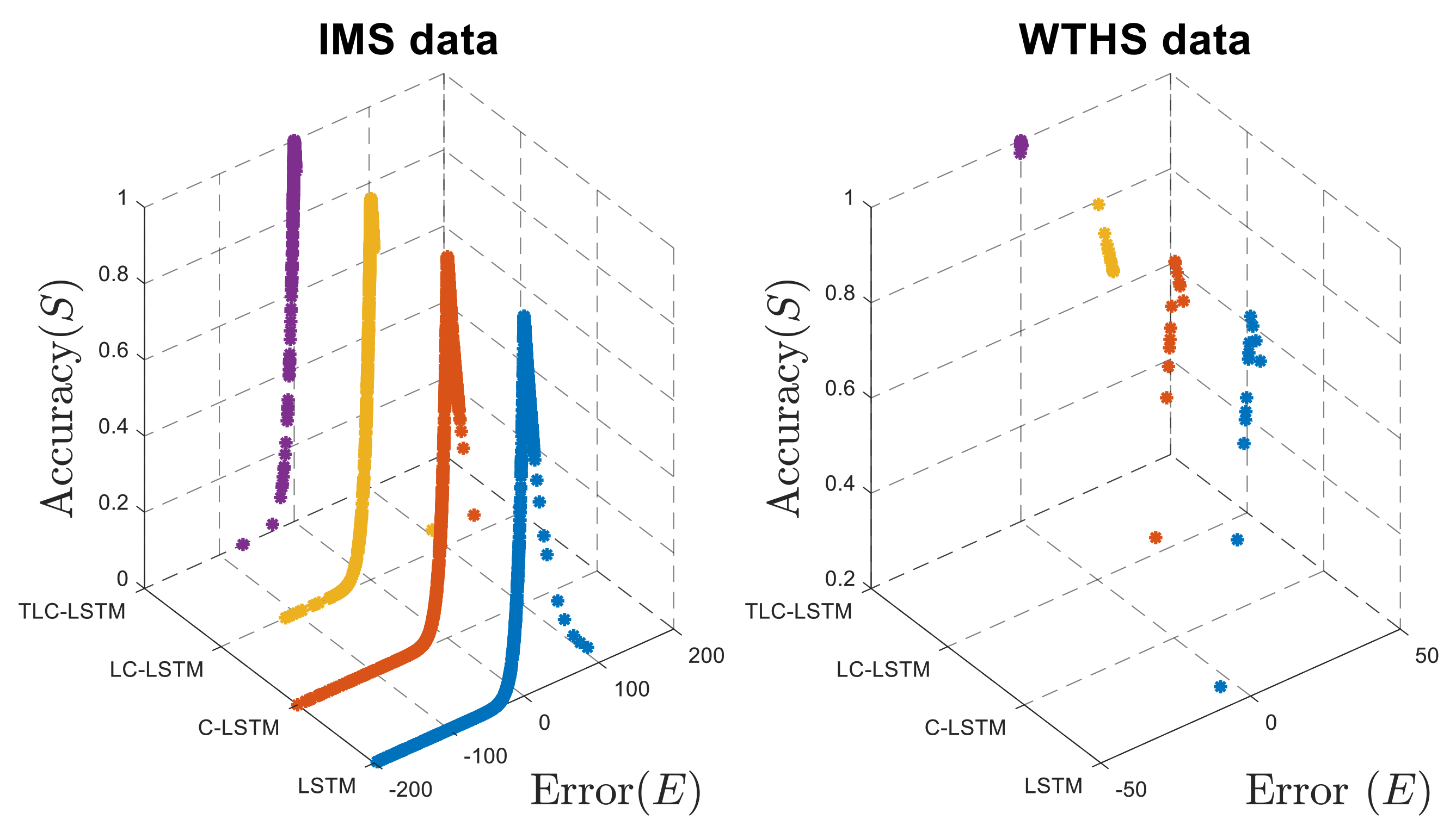
If we used, for instance, any HI accuracy evaluation metric S , such as the one expressed by Equation (16) [34], we will be able to give more information on the accuracy of the learning algorithm by studying the sparseness of the predicted HI values.
S = e ln 0.5 E 5   i f   E 0 e + ln 0.5 E 20   i f   E > 0
where E is an estimation error that can be calculated according to Equation (17).
E = 100 % ( y y ˜ y )
The current accuracy formula was designed to observe the number of errors in the late and early predictions, because later predictions were harmful and the early ones were more demanding on maintenance resources. It also showed the concentration of values towards the value 1: the higher the concentration was, the more accuracy increased.
For instance, Figure 13 explains that all of the designed predictors are most likely early estimators of HI. However, the designed algorithm (TLC-LSTM) has a better approximation and a better accuracy by showing more concentration towards value 1 than the other algorithms.
Table 1 also shows a numerical comparison using the root mean squared error (RMSE) and the accuracy between these studied algorithms and explains Figure 12 and Figure 13 results by showing the strength of designed TLC-LSTM.
In terms of HI predictions, and given that available literature works use different assessment parameters, representations of HI as well as data divisions, it is clearly difficult to collect information needed for comparison (i.e., in a single table). However, if we consider HI curve fit regularity as a criterion, we can definitely consider that our proposal has a higher approximation in comparison to recent works, such as in [15,16,35,36], for WTHS data. Concerning IMS data, the carried-out works, such as in [9,12,13,14,20,37], mainly dealt with the HS classification problem, while in our study, we are proposing HI approximation for IMS data, which can be considered a new contribution in RUL prediction. In addition, the proposed model proves knowledge integration robustness, specifically when no data processing is considered after feature extraction, such as correlation or monotonicity analysis.

3.3. HS Prediction Results

Due to the nature of vibration signals, which resemble consecutively driven sequences in time, the best representation of HI for classes will be the ordinal type of encoding. Therefore, the resulting groups from the GMM were re-sorted and represented with consecutive integers. After that, we followed the same procedures of the previous regression problem to feed the learning samples to the learning models. As a result, the area under the probability curve (AUC) beneath the receiver operating characteristic (ROC) curves of Figure 14 explains the classification capacity of each algorithm. Indeed, we are always able to observe the benefits of each contribution in the classification process. Meanwhile, our proposed algorithm has a larger AUC area, which explains its strong ability to split HS.
Table 2 of classification rates also explains the ability of the new knowledge-driven TLC-LSTM method in health threshold detection by showing more classification accuracy during the testing phase for the unseen data.
Compared to recent data-driven methods, such as [9,10,14,37], our contributions are more general and even clearer as they were able to study both HI and HS at the same time. Therefore, we do not consider numerical proof only as a single parameter of accuracy, for example. In fact, in this work, we have used many metrics (RMSE, accuracy, classification accuracy, and Silhouette coefficient), including graphical interpretations (AUC and ROC), which is strong evidence that supports the ability of the learning algorithm. Additionally, our work also used the same extracted features as an additional contribution, which was considered as one the main contributions of previous works. Moreover, if more additive characteristics are considered for bearing HS splitting, such as those obtained with acoustic signals used in [38], one can find further improved feature space results that ultimately lead to an increased accuracy. Table 3 shows that our followed path is the only one that could provide an optimal conclusion on the RUL among the compared methods.
Generally speaking, with respect to the current knowledge-based framework, the present study proposed a design to solve the problem of incomplete data in the absence of true labels for one-dimensional bearing characteristics. A set of training samples was already obtained from a real life test (WTHS) where further training samples were obtained from an accelerated life test (IMS). The purpose of this hybrid data selection was to collect important patents from real experiences and use them to transfer knowledge to fill the gaps produced by the lake of patterns. In addition, the learning process was managed in reverse to be able to produce an additional generalization in case of insufficient samples due to the small recording period (6s per day).
Bearing measurements have a particular nature, in which a form of time series has been integrated that could be delivered piece by piece. Therefore, the proposed methodology applications in other areas will be clearly possible with any type of time series data with an incomplete list of patterns, as well as with missing labels.

4. Conclusions

In this work, a new approach based on multi-source knowledge was proposed for bearing degradation prognosis. This new scheme combined a stack of autoencoders connected in series specially designed for the integration of labels as a source of knowledge. These autoencoders were used to power data-driven algorithms that integrate C-LSTM for RUL prediction. In addition, this hybridization was maintained to transfer knowledge from a source domain to a specific target domain via TL procedures. This knowledge-driven approach was tested on two different datasets, namely, IMS and WTHS. Unlike previous works, which focused on one of the themes; whether it is HI or HS predictions in a single benchmark, our work studied both in the same experiments. The prediction results were transmitted through numerous measurements, including numerical and graphical interpretation. The evaluation process proved the strength and credibility of the designed algorithm, even when comparing it to a set of recent works. Regarding future works, and in an attempt to reduce algorithmic complexity, one possible trend in this work will be the integration of label seeding inside the C-LSTM itself, rather than the current feature mapping. In addition, one can discuss the use of other approaches that make label mining even easier and increase retrieval capacity by testing other types of feature reconstructions, such as compressed sensing. Additionally, neuron pruning techniques, such as sparse coding, dropout, and contractive autoencoding, could be involved to keep only important meaningful descriptions from learning samples.

Author Contributions

Conceptualization, T.B.; methodology, T.B., M.B., and L.-H.M.; software, T.B.; validation, T.B., M.B., and L.-H.M.; formal analysis, T.B., M.B., and L.-H.M.; investigation, T.B.; writing—original draft preparation, T.B.; writing—review and editing, T.B., M.B., and L.-H.M.; supervision, M.B. and L.-H.M. All authors have read and agreed to the published version of the manuscript.

Funding

This research received no external funding.

Institutional Review Board Statement

Not applicable.

Informed Consent Statement

Not applicable.

Data Availability Statement

Conflicts of Interest

The authors declare no conflict of interest.

References

  1. Berghout, T.; Mouss, L.H.; Bentrcia, T.; Elbouchikhi, E.; Benbouzid, M. A deep supervised learning approach for condition-based maintenance of naval propulsion systems. Ocean. Eng. 2021, 221, 108525. [Google Scholar] [CrossRef]
  2. Peng, J.; Zheng, Z.; Zhang, X.; Deng, K.; Gao, K.; Li, H.; Chen, B.; Yang, Y.; Huang, Z. A data-driven method with feature enhancement and adaptive optimization for lithium-ion battery remaining useful life prediction. Energies 2020, 13, 752. [Google Scholar] [CrossRef] [Green Version]
  3. Lei, Y. Remaining useful life prediction. Intelligent Fault Diagnosis and Remaining Useful Life Prediction of Rotating Machinery; Elsevier BV: Oxford, UK, 2017; pp. 281–358. [Google Scholar]
  4. Lei, Y.; Li, N.; Guo, L.; Li, N.; Yan, T.; Lin, J. Machinery health prognostics: A systematic review from data acquisition to RUL prediction. Mech. Syst. Signal. Process. 2018, 104, 799–834. [Google Scholar] [CrossRef]
  5. Khamoudj, C.E.; Benbouzid-Si Tayeb, F.; Benatchba, K.; Benbouzid, M.; Djaafri, A. A Learning Variable Neighborhood Search Approach for Induction Machines Bearing Failures Detection and Diagnosis. Energies 2020, 13, 2953. [Google Scholar] [CrossRef]
  6. Yan, M.; Wang, X.; Wang, B.; Chang, M.; Muhammad, I. Bearing remaining useful life prediction using support vector machine and hybrid degradation tracking model. ISA Trans. 2020, 98, 471–482. [Google Scholar] [CrossRef]
  7. Li, X. Deep learning-based remaining useful life estimation of bearings using multi-scale feature extraction. Reliab. Eng. Syst. Saf. 2019, 182, 208–218. [Google Scholar] [CrossRef]
  8. Sun, S.; Przystupa, K.; Wei, M.; Yu, H.; Ye, Z.; Kochan, O. Fast bearing fault diagnosis of rolling element using Lévy Moth-Flame optimization algorithm and Naive Bayes. Eksploat. I Niezawodn. 2020, 22, 730–740. [Google Scholar] [CrossRef]
  9. Ben Ali, J.; Saidi, L.; Mouelhi, A.; Chebel-Morello, B.; Fnaiech, F. Linear feature selection and classification using PNN and SFAM neural networks for a nearly online diagnosis of bearing naturally progressing degradations. Eng. Appl. Artif. Intell. 2015, 42, 67–81. [Google Scholar] [CrossRef] [Green Version]
  10. Ben Ali, J.; Harrath, S.; Bechhoefer, E.; Benbouzid, M. Online automatic diagnosis of wind turbine bearings progressive degradations under real experimental conditions based on unsupervised machine learning Online automatic diagnosis of wind turbine bearings progressive degradations under real experimental con. Appl. Acoust. 2018, 132, 167–181. [Google Scholar] [CrossRef]
  11. Qiu, H.; Lee, J.; Lin, J.; Yu, G. Wavelet filter-based weak signature detection method and its application on rolling element bearing prognostics. J. Sound. Vib. 2006, 289, 1066–1090. [Google Scholar] [CrossRef]
  12. Han, S.; Oh, S.; Jeong, J. Bearing Fault Diagnosis Based on Multiscale Convolutional Neural Network Using Data Augmentation. J. Sens. 2021, 2021, 6699637. [Google Scholar] [CrossRef]
  13. Moshrefzadeh, A. Condition monitoring and intelligent diagnosis of rolling element bearings under constant/variable load and speed conditions. Mech. Syst. Signal. Process. 2021, 149, 107153. [Google Scholar] [CrossRef]
  14. Zareapoor, M.; Shamsolmoali, P.; Yang, J. Oversampling adversarial network for class-imbalanced fault diagnosis. Mech. Syst. Signal. Process. 2021, 149, 107175. [Google Scholar] [CrossRef]
  15. Saidi, L.; Ben Ali, J.; Bechhoefer, E.; Benbouzid, M. Wind turbine high-speed shaft bearings health prognosis through a spectral Kurtosis-derived indices and SVR. Appl. Acoust. 2017, 120, 1–8. [Google Scholar] [CrossRef]
  16. Meddour, I.; Messekher, S.E.; Younes, R.; Yallese, M.A. Selection of bearing health indicator by GRA for ANFIS-based forecasting of remaining useful life. J. Braz. Soc. Mech. Sci. Eng. 2021, 43, 144. [Google Scholar] [CrossRef]
  17. Li, X.; Zhang, W.; Ma, H.; Luo, Z.; Li, X. Data alignments in machinery remaining useful life prediction using deep adversarial neural networks. Knowl.-Based Syst. 2020, 197, 105843. [Google Scholar] [CrossRef]
  18. Wang, J.; Liang, Y.; Zheng, Y.; Gao, R.X.; Zhang, F. An integrated fault diagnosis and prognosis approach for predictive maintenance of wind turbine bearing with limited samples. Renew. Energy 2020, 145, 642–650. [Google Scholar] [CrossRef]
  19. Huang, G.; Zhang, Y.; Ou, J. Transfer remaining useful life estimation of bearing using depth-wise separable convolution recurrent network. Measurement 2021, 176, 109090. [Google Scholar] [CrossRef]
  20. Kim, M.; Uk, J.; Lee, J.; Youn, B.D.; Ha, J. A Domain Adaptation with Semantic Clustering (DASC) method for fault diagnosis of rotating machinery. ISA Trans. 2021, 1. [Google Scholar] [CrossRef]
  21. Cheng, H.; Kong, X.; Chen, G.; Wang, Q.; Wang, R. Transferable convolutional neural network based remaining useful life prediction of bearing under multiple failure behaviors. Meas. J. Int. Meas. Confed. 2021, 168, 108286. [Google Scholar] [CrossRef]
  22. Zhuang, F.; Qi, Z.; Duan, K.; Xi, D.; Zhu, Y.; Zhu, H.; Xiong, H.; He, Q. A comprehensive survey on transfer learning. Proc. IEEE 2020, 109, 43–76. [Google Scholar] [CrossRef]
  23. Sánchez-Morales, A.; Sancho-Gómez, J.-L.; Figueiras-Vidal, A.R. Exploiting label information to improve auto-encoding based classifiers. Neurocomputing 2019, 370, 104–108. [Google Scholar] [CrossRef]
  24. Sánchez-Morales, A.; Sancho-Gómez, J.L.; Figueiras-Vidal, A.R. Complete autoencoders for classification with missing values. Neural Comput. Appl. 2020, 33, 1951–1957. [Google Scholar] [CrossRef]
  25. Berghout, T. A New Health Assessment Prediction Approach: Multi-Scale Ensemble Extreme Learning Machine. Preprints 2020. [Google Scholar] [CrossRef]
  26. Tovar, M.; Robles, M.; Rashid, F. PV Power Prediction, Using CNN-LSTM Hybrid Neural Network Model. Case of Study: Temixco-Morelos, México. Energies 2020, 13, 6512. [Google Scholar] [CrossRef]
  27. NASA Prognostics Center of Excellence. Available online: https://ti.arc.nasa.gov/tech/dash/groups/pcoe/prognostic-data-repository/#turbofan (accessed on 20 March 2021).
  28. Mathworks Wind Turbine High-Speed Bearing Prognosis. Available online: https://www.mathworks.com/help/predmaint/ug/wind-turbine-high-speed-bearing-prognosis.html (accessed on 21 March 2021).
  29. Panić, B.; Klemenc, J.; Nagode, M. Gaussian Mixture Model Based Classification Revisited: Application to the Bearing Fault Classification. Stroj. Vestn.-J. Mech. Eng. 2020, 66, 215–226. [Google Scholar] [CrossRef] [Green Version]
  30. He, Z.; Zhang, X.; Liu, C.; Han, T. Fault Prognostics for Photovoltaic Inverter Based on Fast Clustering Algorithm and Gaussian Mixture Model. Energies 2020, 13, 4901. [Google Scholar] [CrossRef]
  31. Rousseeuw, P.J. Silhouettes: A graphical aid to the interpretation and validation of cluster analysis. J. Comput. Appl. Math. 1987, 20, 53–65. [Google Scholar] [CrossRef] [Green Version]
  32. Berghout, T.; Mouss, L.; Kadri, O.; Saïdi, L.; Benbouzid, M. Aircraft Engines Remaining Useful Life Prediction with an Improved Online Sequential Extreme Learning Machine. Appl. Sci. 2020, 10, 1062. [Google Scholar] [CrossRef] [Green Version]
  33. Schmidhuber, J. Deep Learning in neural networks: An overview. Neural Netw. 2015, 61, 85–117. [Google Scholar] [CrossRef] [Green Version]
  34. Yoo, Y.; Baek, J.G. A novel image feature for the remaining useful lifetime prediction of bearings based on continuous wavelet transform and convolutional neural network. Appl. Sci. 2018, 8, 1102. [Google Scholar] [CrossRef] [Green Version]
  35. Elforjani, M.; Shanbr, S.; Bechhoefer, E. Detection of faulty high speed wind turbine bearing using signal intensity estimator technique. Wind. Energy 2018, 21, 53–69. [Google Scholar] [CrossRef]
  36. Elasha, F.; Shanbr, S.; Li, X.; Mba, D. Prognosis of a wind turbine gearbox bearing using supervised machine learning. Sensors 2019, 19, 3092. [Google Scholar] [CrossRef] [PubMed] [Green Version]
  37. Mao, W.; Feng, W.; Liu, Y.; Zhang, D.; Liang, X. A new deep auto-encoder method with fusing discriminant information for bearing fault diagnosis. Mech. Syst. Signal. Process. 2021, 150, 107233. [Google Scholar] [CrossRef]
  38. Glowacz, A. Acoustic fault analysis of three commutator motors. Mech. Syst. Signal. Process. 2019, 133, 106226. [Google Scholar] [CrossRef]
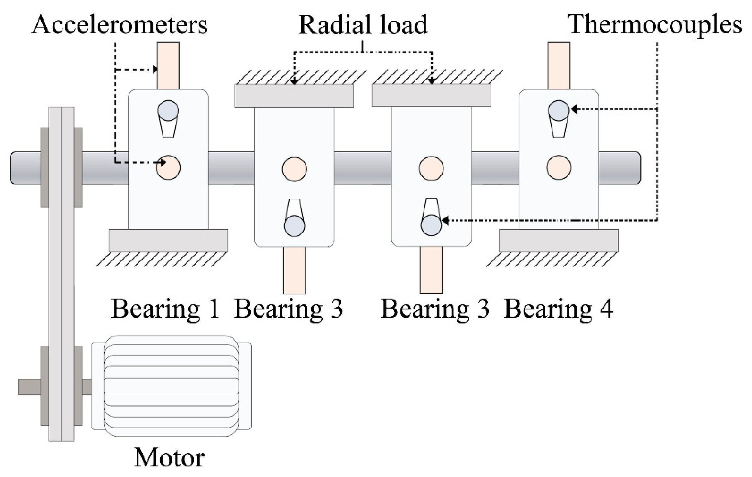
Figure 1. IMS bearing tests experimental setup.
Energies 14 02163 g001
Figure 2. Recorded raw data from IMS bearing experimental platform.
Energies 14 02163 g002
Figure 3. (a) Position of the main bearings in a wind turbine. (b) Studied bearing type and its dimensions.
Energies 14 02163 g003
Figure 4. Run-to-failure vibration sensor measurements of WTHS.
Energies 14 02163 g004
Figure 5. Adopted methodology during health assessment model development.
Energies 14 02163 g005
Figure 6. Final prepared versions of the studied datasets.
Energies 14 02163 g006
Figure 7. Given health indexes for each deterioration path.
Energies 14 02163 g007
Figure 8. Results of health stage (HS) splitting by Gaussian mixture model (GMM).
Energies 14 02163 g008
Figure 9. Process of integrating labels into a robust denoising scheme.
Energies 14 02163 g009
Figure 10. Data-driven approach for both learning and knowledge transfer. LSTM, long–short-term memory.
Energies 14 02163 g010
Figure 11. Label recovering characteristics.
Energies 14 02163 g011
Figure 12. Health index (HI) curve fittings results.
Energies 14 02163 g012
Figure 13. Studied algorithm accuracy.
Energies 14 02163 g013
Figure 14. HI classifiers ofarea under the probability curve beneath the receiver operating characteristic (AUC-ROC) curves.
Energies 14 02163 g014
Table 1. Numerical evaluation of the studied algorithms.
WTHS Data
AlgorithmRMSE Accuracy S
LSTM0.03050.8094
C-LSTM0.02170.8477
LC-LSTM0.01320.8679
TLC-LSTM0.00170.9921
IMS Data
LSTM0.21410.5883
C-LSTM0.10100.7259
LC-LSTM0.01850.8844
TLC-LSTM0.00650.9636
Table 2. Classification rates of HS detectors.
Dataset
AlgorithmIMSWTHS
LSTM0.84363%0.90000%
C-LSTM0.96196%0.95000%
LC-LSTM0.96117%0.95000%
TLC-LSTM0.96856%0.95000%
Table 3. Comparison with advanced state of the art methods. RMSE, root mean squared error; IMS, intelligent maintenance systems.
WTHS Data
ApproachHSHIHI Metrics HS Metrics
Saidi, L. et al. [15]Curve fitting only
Meddour, I et al. [16]Average percentage error (%) and curve fitting
Elforjani, M. et al. [35]Average percentage error (%) and curve fitting
Elasha, F. et al. [36]Sum square error results
Ben Ali, J. [10]Classification accuracy only
TLC-LSTMRMSE, accuracy formula (equation (16)) and curve fittingClassification accuracy, data scatters, ROC curves, AUC and silhouette coefficient
IMS data
Ben Ali, J. et al. [9]Classification accuracy and ROC curves
Han, S. et al. [12]F1 score and confusion matrix
Moshrefzadeh, A. et al. [13]Classification accuracy and confusion matrix
Zareapoor, M. et al. [14]Precision, Recall, FAM (average of AUC, MCC, and F1-measure)
Mao, W. et al. [37]Classification accuracy and confusion matrix
TLC-LSTMRMSE, accuracy formula (equation (16)) and curve fittingClassification accuracy, data scatters, ROC curves, AUC and silhouette coefficient
Publisher’s Note: MDPI stays neutral with regard to jurisdictional claims in published maps and institutional affiliations.